Low frequency radio astronomy from the moon: cosmic reionization and more

Abstract

We discuss low frequency radio astronomy from the moon, predominantly in the context of studying the neutral intergalactic medium during cosmic reionization using the HI 21cm line of neutral hydrogen. The epoch of reionization is the next frontier in observational cosmology, and HI 21cm studies are recognized as the most direct probe of this key epoch in cosmic structure formation. Current constraints on reionization indicate that the redshifted HI 21cm signals will likely be in the range of 100 MHz to 180 MHz, with the pre-reionization signal going to as low as 10 MHz. The primary observational challenges to these studies are:

• ionospheric phase fluctuations

• terrestrial radio frequency interference

• Galactic and extragalactic foreground radiation.

Going to the far side of the moon removes the first two of these challenges. Moreover, a low frequency telescope will be relatively easy to deploy and maintain on the moon, at least compared to other, higher frequency telescopes. We discuss the potential 21cm signals from reionization, and beyond, and the telescope specifications needed to measure these signals. We then describe ground-based projects currently underway to study the HI 21cm signal from cosmic reionization. We include a brief discussion of other very low frequency science enabled by being outside the Earth’s ionosphere.

The near-term ground-based projects will act as path-finders for a potential future low frequency radio telescope on the moon, both in terms of initial scientific results on the HI 21cm signal from cosmic reionization, and in terms of the telescope design and observing techniques required to meet the stringent sensitivity and dynamic range requirements. If it is found that the terrestrial interference environment, or ionospheric phase fluctuations, preclude ground-based studies of reionization, then it becomes imperative to locate future telescopes on the far side of the moon. Besides pursuing these path-finder reionization telescopes, we recommend a number of near-term studies that could help pave the way for low frequency astronomy on the moon.

1 Introduction

There is long standing interest in building a low frequency radio telescope on the far side of the moon (Gorgolewski 1965; Burke 1985; Kuiper et al. 1990; Burns & Asbell 1991; Woan et al. 1997). The reasons are clear (section 2): no ionosphere, and sheilding from terrestrial radio frequency interference (RFI). Two factors have acted to rekindle interest in low frequency radio astronomy from moon. First, scientifically, efforts to study cosmic reionization through the redshifted HI 21cm line have spurred numerous ground-based low frequency projects (section 3). And second is the new NASA initiative to return Man to the moon, and beyond.

In this paper we discuss the advantages of building a radio telescope on the far side of the moon. We present the primary scientific driver in low frequency astronomy today, namely HI 21cm studies of cosmic reionization, and discuss some of the near-term ground-based telescopes being designed for these studies. We also present other very low frequency science programs that are enabled by going to the moon. We close with a few recommendations for near-term studies that might prove useful for planning a low frequency lunar telescope.

2 Why the moon for low frequency radio astronomy?

We start with the main advantages for considering the far side of the moon for a low frequency radio telescope. Low frequencies, in the context of this paper, means frequencies, $\nu<200$MHz ($\lambda>1.5$m). In this regime it becomes cheaper, and possibly more effective, to build arrays of dipoles, which are electronically steered through phasing of the dipole elements, as opposed to steerable parabolic reflectors.

• Ionospheric opacity: The plasma frequency of the Earth’s ionosphere varies between roughly 10MHz and 20MHz, making the ionosphere optically thick at lower frequencies. For the reionization experiments discussed in Section 3, the relevant frequency range is $>30$ MHz, hence ionospheric opacity is not an issue. We discuss in Section 4 some very low frequency science, in the range 0.1 MHz and 10MHz, that are enabled by going to the moon.

• Ionospheric phase errors: The fluctuating ionosphere also cause variations in electronic path-length, which increase as $\nu^{-2}$. Hence, fluctuations in the electron content of the ionosphere will preclude low frequency imaging with synthesis arrays unless a correction can be made for electronic phase variations due to the varying ionosphere. Figure 1 shows an example of ionospheric phase errors on source positions using VLA data at 74 MHz (Cotton et al. 2004; Lane et al. 2004). Positions of five sources are shown for a series of snap shot images over 10 hours. A number of interesting phenomena can be seen. First, the sources are slowly moving in position over time, by $\pm 50"$ over timescales of hours. These position shifts reflect the changing electronic path-length due to the fluctuating ionosphere (ie. tilts in the incoming wavefront due to propagation delay). Second, the individual sources move roughly independently. This is a demonstration of the ’isoplanatic patch’ problem, ie. the excess electrical path-length is different in different directions. At 74 MHz, the typical coherent patch size is about 3^o to 4^o. Celestial calibrators further than this distance from a target source no longer give a valid solution for the combined instrumental and propagation delay term required to image the target source. And third, at the end of the observation there occurs an ionospheric storm, or traveling ionospheric disturbance, which effectively precludes coherent imaging during the event.

  New wide field self-calibration techniques, involving multiple phase solutions over the field, or a ‘rubber screen’ phase model (Cotton et al. 2004; Hopkins et al. 2003), are being developed that should allow for self-calibration over wide fields. Again, the moon presents a clear advantage in this regard, being beyond the Earth’s ionosphere.

• Terrestrial radio frequency interference (RFI): Another problem facing low frequency radio astronomy is terrestrial (man-made) interference. Frequencies $<200$MHZ are not protected bands, and commercial allocations include everything from broadcast radio and television, to fixed and mobile communications. At the lowest frequencies ($<1$MHz) the Earth’s auroral emission dominates.

  Many groups are pursuing methods for RFI mitigation and excision (see Ellingson 2004). These include: (i) using a reference horn, or one beam of a phased array, for constant monitoring of known, strong, RFI signals, (ii) conversely, arranging interferometric phases to produce a null at the position of the RFI source, and (iii) real-time RFI excision using advanced filtering techniques in time and frequency, of digitized signals both pre- and post-correlation. The latter requires very high dynamic range (many bit sampling), and very high frequency and time resolution.

  In the end, the most effective means of reducing interference is to go to the remotest sites. A number of the near-term low frequency path-finder telescopes (see Section 4), have selected sites in remote regions of Western Australia and China, because of known low RFI environments.

  Clearly the best location to avoid terrestrial interference is the far-side of the moon. Figure 2 shows the effect of the lunar radio shadow on the RAE2 lunar orbiter (Alexander et al. 1975). This orbiter had a low frequency ($<10$MHz) radio receiver. The figure shows complete blockage of the Earth’s auroral emission during immersion. Note that this interference blockage is the key argument for the far side of the moon, as opposed to a free-flying space radio telescope.

• Ease of deployment and maintenance: While not a scientific rationale, it should be pointed out that a low frequency telescope may be the easiest astronomical facility to deploy and maintain on the moon. The antennas and electronics are high tolerance, with wavelengths $>1.5$m and system noise characteristics dominated by the Galactic foreground radiation. Deployment could be automated, using either javelin deployment (EADS/ASTRON), rollout of thin polyimide films with metalic deposits (ROLSS; Lazio et al. 2006), inflatable dipoles (LUDAR; Corbin et al. 2005), or deployment by rovers. Likewise, being a phased array, low frequency telescopes are electronically steered, and hence have no moving parts. Lastly, there is no potential difficulty with lunar dust affecting the optics.

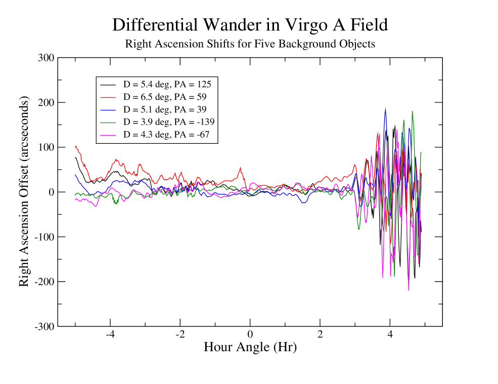
Figure 1: The positions of five sources in the Virgo A field at 74 MHz observed with the VLA over 10 hours (Cotton et al. 2004; Lane et al. 2004). The source positions vary with time due to fluctuations in the electronic path-length through the ionosphere.

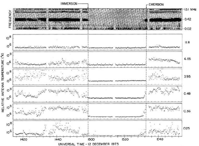
Figure 2: Radio power received by the lunar orbiting radio astronomy explorer satellite in 1973 (RAE2; Alexander et al. 1975). The power is dominated by the Earth’s auroral emission except during immersion, when the Earth is totally blocked by the moon.

3 Cosmic Reionization

3.1 The HI 21cm signal

Cosmic reionization corresponds to the transition from a fully neutral intergalactic medium (IGM) to an (almost) fully ionized IGM caused by the UV radiation from the first stars and blackholes. Reionization is a key benchmark in cosmic structure formation, indicating the formation of the first luminous objects. Reionization, and the preceding ’dark ages’, represent the last of the major phases of cosmic evolution to explore. Recent observations of the Gunn-Peterson effect, ie. Ly-$\alpha$ absorption by the neutral IGM, toward the most distant quasars ($z\sim 6$), and the large scale polarization of the CMB, have set the first constraints on the epoch of reionization. These data, coupled with the study of high-$z$ galaxy populations and other observations, suggest that reionization was a complex process, with significant variance in both space and time, starting perhaps as high as $z\sim 14$, with the last vestiges of the the neutral IGM being etched-away by $z\sim 6$ (Fan et al. 2006;, Ciardi & Ferrara 2005; Loeb 2006).

The most direct and incisive means of studying cosmic reionization is through the 21cm line of neutral Hydrogen (Furlanetto et al. 2006). The study of HI 21cm emission from cosmic reionization entails the study of large scale structure (LSS). During this epoch the entire IGM may be neutral, and the LSS in question is not simply mass clustering, but involves a combination of structure in cosmic density, neutral fraction, and HI excitation temperature (Loeb 2006). Hence, HI 21cm observations are potentially the ‘richest of all cosmological data sets’ (Loeb & Zaldarriaga 2004). Information about the physics of cosmology (involving the initial perturbations from inflation and the matter content of the universe) can be separated from the astronomical aspects (involving galaxy formation) through the line-of-sight anisotropy imprinted by peculiar velocities on the power-spectrum of 21cm brightness fluctuations (Barkana & Loeb 2005a). We briefly describe a few of the potential HI 21cm signatures of cosmic reionization.

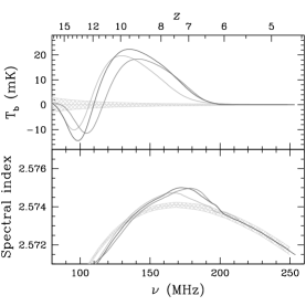
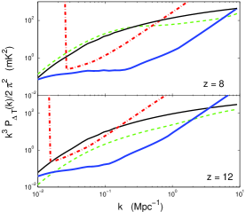
Figure 3: Left: Global (all sky) HI signal from reionization (Gnedin & Shaver 2003). The shaded region shows the expected thermal noise in a carefully controlled experiment. Center: Predicted HI 21cm brightness temperature power spectrum (in log bins) at redshifts 8 and 12 (Mcquinn et al. 2006). The thin black line shows the signal when density fluctuations dominate. The dashed green line shows the predicted signal for ionization fraction, $\bar{x}_{i}=0.2$ at $z=12$, and $\bar{x}_{i}=0.6$ at $z=8$, in the Furlanetto et al. (2004) semi-analytic model. The thick blue line shows the Square Kilometer Array (SKA; Carilli & Rawlings 2004) sensitivity in 1000hrs. The thick red dot-dash show the sensitivity of the path-finder experiment LOFAR. The cutoff at low k is set by the primary beam. Right: The simulated SKA spectrum of a radio continuum source at $z=10$ (Carilli et al. 2002). The straight line is the intrinsic power law (synchrotron) spectrum of the source. The noise curve shows the effect of the 21cm line in the neutral IGM, including noise expected for the SKA in a 100 hour integration.

• Global signal: The left panel in Figure 3 shows the latest predictions of the global (all sky) increase in the background temperature due to the HI 21cm line from the neutral IGM (Gnedin & Shaver 2003). The predicted HI signal peaks at roughly 20 mK above the foreground at $z\sim 10$. At higher redshift, prior to IGM warming, the kinetic temperature of the IGM will be colder than the CMB temperature. In this case, Ly$\alpha$ emission from the first luminous objects can couple the gas kinetic temperature to the HI spin temperature through the resonant scattering of Ly$\alpha$ photons (Wouthuysen 1952; Field 1959). In this case, the HI will be seen in absorption against the CMB. Since this is an all sky signal, the sensitivity of the experiment is independent of telescope collecting area, and the experiment can be done using small area telescopes at low frequency, with very well controlled frequency response (Rogers & Bowman, in prep; Subrahmanyan, in prep). Note that the line signal is only $\sim 10^{-4}$ that of the mean foreground continuum emission at $\sim 150$ MHz (see Section 3.2).

• Power spectra: The middle panel in Figure 3 shows the predicted power spectrum of spatial fluctuations in the sky brightness temperature due to the HI 21cm line (Mcquinn et al. 2006). For power spectral analyses the sensitivity is greatly enhanced relative to direct imaging due to the fact that the universe is isotropic, and hence one can average the measurements in annuli in the Fourier (uv) domain, ie. the statistics of fluctuations along an annulus in the uv-plane are equivalent. Moreover, unlike the CMB, HI line studies provide spatial and redshift information, and hence the power spectral analysis can be performed in three dimensions. The rms fluctuations at $z=10$ peak at about 10 mK rms on scales $\ell\sim 5000$ ($\sim 2^{\prime}$).

• Absorption toward discrete radio sources: A interesting alternative to emission studies is the possibility of studying smaller scale structure in the neutral IGM by looking for HI 21cm absorption toward the first radio-loud objects (AGN, star forming galaxies, GRBs) (Carilli et al. 2002). The right panel of Figure 3 shows the predicted HI 21cm absorption signal toward a high redshift radio source due to the ‘cosmic web’ prior to reionization, based on numerical simulations. For a source at $z=10$, these simulations predict an average optical depth due to 21cm absorption of about 1$\%$, corresponding to the ‘radio Gunn-Peterson effect’, and about five narrow (few km/s) absorption lines per MHz with optical depths of a few to 10$\%$. These latter lines are equivalent to the Ly $\alpha$ forest seen after reionization. Furlanetto & Loeb (2002) predict a similar HI 21cm absorption line density due to gas in minihalos, as that expected for the 21cm forest. This absorption experiment may be the easiest of the HI 21cm probes of reionization to perform, since it entails absorption against a high brightness temperature object, and hence is less affected by 3D dynamic range issues, and it can use long baselines, which are less susceptable to interference. However, the experiment is predicated on the existence of radio sources at these during reionization. This question has been considered in detail by Carilli et al. (2002), Haiman et al. (2004), and Jarvis & Rawlings (2005). They show that current models of radio-loud AGN evolution predict between 0.05 and 1 radio sources per square degree at $z>6$ with $\rm S_{150MHz}\geq 6$ mJy, adequate for reionization HI 21cm absorption studies with the Square Kilometer Array (SKA).

• Tomography: Figure 4 shows the expected evolution of the HI 21cm signal during reionization based on numerical simulations (Zaldarriaga et al. 2004). In this simulation, the HII regions caused by galaxy formation are seen in the redshift range $z\sim 8$ to 10, reaching scales up to 2^′ (frequency widths $\sim 0.3$ MHz $\sim 0.5$ Mpc physical size). These regions appear as ’holes in the sky’, with (negative) brightness temperatures up to 20 mK. This corresponds to 5$\mu$Jy beam^-1 in a 2^′ beam at 140 MHz. Only a full square kilometer of collecting will be able to perform the 3D tomographic imaging of the typical structures during reionization (Section 3.3).

• Cosmic Stromgren spheres: While direct detection of the typical structure of HI and HII regions may be out of reach of the path-finder telescopes (Section 3.2), there is a chance that even these first generation telescopes will be able to detect the rare, very large scale HII regions associated with luminous quasars near the end of reionization. The expected signal is $\sim 20$mK $\times~{}x_{HI}$ on scales $\sim 10^{\prime}$ to 15^′, with line widths $\sim 1$ to 2 MHz (Wyithe et al. 2005), where $x_{HI}$ is the IGM neutral fraction, by volume. This corresponds to 0.5 $\times~{}x_{HI}$ mJy beam^-1, for a 15^′ beam at $z\sim 6$ to 7.

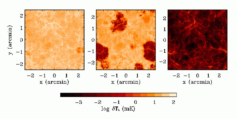
Figure 4: The simulated HI 21cm brightness temperature distribution during reionization at $z=12$, 9, 7 (left to right; Zaldarriaga et al. 2004).

3.2 Sensitivities, foregrounds, and telescope requirements

A number of groups have calculated the expected HI 21cm signals from cosmic reionization, including large bubbles associated with bright quasars, and clustering of star forming galaxies (Zaldarriaga et al. 2004; Wyithe et al. 2005; Mellema et al. 2006; Madau et al. 1997). The larger structures will vary from a few to 15 arcmin in size, with a depth of $20\times~{}x_{HI}$ mK. For demonstrative purposes, we assume a target signal for detection of 10mK and 10^′ in size at $z=8$. This implies an observing frequency of $\nu=158$MHz, or observing wavelength, $\lambda=1.9$m. For reference, at $z\sim 8$, 10^′ = 3.2 Mpc physical size, or in co-moving coordinates 10^′ = 3.2/(1+z) = 0.36 Mpc co-moving, and in terms of the Hubble expansion, 3.2 Mpc (physical) = 1.6 MHz. The angular size of 10^′ corresponds to a baseline length of 650m at 158MHz.

The relationship between brightness temperature and flux density is given by:

$$\rm T_{B}=1360{{S_{\nu}}\over{\theta^{2}}}\lambda^{2}~{}K$$

where S_ν is the flux density in Jy, $\theta$ is the angular size, in arcseconds, and $\lambda$ is the observing wavelength in centimeters. For reference, a 10mK signal at $\lambda=1.9$m and $\theta=10^{\prime}$ corresponds to 73$\mu$Jy.

Sensitivity: The sensitivity of a radio telescope is given by the radiometry equation:

$$\rm rms=3000{{T_{sys}}\over{\epsilon NA}}(\Delta\nu~{}t)^{-1/2}~{}Jy$$

where $\epsilon$ is the antenna efficiency, N is the number of antennas, A is the physical collecting area of each antenna, in m², $\Delta\nu$ is the bandwidth (Hz), and t is the integration time (seconds). The system temperature, $\rm T_{sys}$, is the sum of the receiver temperature, which we assume is of order 100 K, and the contribution from the sky foreground. The sky is about 90% diffuse Galactic emission, and 10% extragalactic radio sources. In the coldest regions, the sky contributes:

$$\rm T_{sky}\sim 100({{\nu}\over{200MHz}})^{-2.8}$$

or about 200K at 158MHz. In general, at low frequencies the sky brightness dominates the system temperature. Note that the expected signal is roughly $2\times 10^{4}$ times weaker than the diffuse foreground brightness temperature, even in the coldest regions of the sky.

What collecting area is needed to detect the 73$\mu$Jy signal at 4$\sigma$ at 158MHz in 1000 hrs, assuming a bandwidth of 1.6MHz and an efficiency of 60%? The required area = $3.4\times 10^{4}$ m². This corresponds to roughly 9500 dipoles, assuming each dipole collecting area is of order $\lambda^{2}$.

The path-finder arrays will likely not have the sensitivity to perform true 3D ’tomographic imaging’ of the HI 21cm signal during reionization. These arrays are being designed to study the statistical signal, ie. the power spectrum of brightness temperature fluctuations due to the structure of the neutral IGM, in a manner similar to the COBE statistical detection of CMB brightness temperature fluctuations (see section 3.1). The sensitivity for these near-term arrays to study the power spectrum of the neutral IGM during reionization is shown in Figure 3.

Dynamic range: Besides raw sensitivity, a significant challenge to wide field, low frequency interferometric imaging is dynamic range, set by residual calibration errors and incomplete Fourier spacing coverage. Besides the diffuse Galactic foreground, every field will have bright extragalactic and Galactic continuum sources.

As a rough estimate for the number of sources expected in a given field, we adopt a field size of $20^{o}\times 20^{o}$, corresponding to the field of view of a receptor ’tile’ of $3\times 3$ dipoles. Using the 3C catalog, the bright source counts at 1.9m follows roughly:

$$\rm N(>S)=0.29~{}S^{-1.36}~{}deg^{-2}$$

where N is the number of sources per deg^-2 brighter than S in Jy. Hence, in a typical 400 deg² region, we expect one source brighter than 34 Jy at 158 MHz.

The dynamic range requirement $\equiv$ (Peak in field)/(rms required). The rms required for a 4$\sigma$ detection = 73/4 = 18 $\mu$Jy. Hence, the DNR = 34 Jy/18 $\mu$Jy = $1.9\times 10^{6}$.

Perley (1999; equ. 13-8) derives the dynamic range limit for a synthesis array assuming ’random’ antenna based phase errors, $\Delta\phi$ (in radians):

$$\rm DNR\sim{{N}\over{2^{1/2}\Delta\phi}}$$

where, again, N is the number of elements in the array. Assuming 9500 dipoles grouped in 3x3 tiles implies N = 1055 elements. The requirement then on the phase calibration is: $\Delta\phi<0.023^{o}$.

There have been numerous studies on how to separate the HI 21cm signal from the foreground continuum emission at the required levels. All these techniques rely on the spectral nature of the HI signal. The foreground emission is syncrotron radiation, and hence shows at most gradual changes with frequency on scales of tens to hundreds of MHz. The HI signal is a resonant spectral line, and will have structure on scales of kHz to a few MHz. A number of complimentary approaches have been presented for foreground removal (Morales, Bowman, & Hewitt 2005). Gnedin & Shaver (2003) and Wang et al (2005) consider fitting smooth spectral models (power-laws or low order polynomials in log space) to the observed visibilities or images. Morales & Hewitt (2003) and Morales (2004) present a 3D Fourier analysis of the measured visibilities, where the third dimension is frequency. The different symmetries in this 3D space for the signal arising from the noise-like HI emission, versus the smooth (in frequency) foreground emission, can be a powerful means of differentiating between foreground emission and the reioniation HI line signal. Santos et al. (2005), Bharadwaj & Ali (2005), and Zaldarriaga et al. (2004) perform a similar analysis, only in the complementary Fourier space, meaning cross correlation of spectral channels. They show that the 21cm signal will effectively decorrelate for channel separations $>1$ MHz, while the foregrounds do not. The overall conclusion of these methods is that spectral decomposition should be adequate to separate synchrotron foregrounds from the HI 21cm signal from reionization at the mK level, as long as residual, at least in the absence of residual significant, frequency dependent calibration errors.

3.3 Telescopes

Table 1 summarizes the current experiments under construction to study the HI 21cm signal from cosmic reionization. These experiments vary from single dipole antennas to study the all-sky signal, to 10,000 dipole arrays to perform the power spectral analysis, and potentially to image the largest structures during reionization (eg. the quasar Stromgren spheres).

Most of the experiments have a few to 10% of the collecting area of the SKA, and there are many common features. First, they all rely on some form of a wide-band dipole or spiral antenna, eg. log-periodic yagis, sleeve dipoles, or bow-ties, with steering of the array response through electronic phasing of the elements. Second, the front-end electronics are relatively simple (amplifier/balun), since the system performance is dominated by the sky brightness temperature. Third, most rely on a grouping of dipoles into ’tiles’ or ’stations’, to decrease the field-of-view, and to decrease the data rate into the correlator to a managable level. And forth, the large number of array elements, and the need for wide-field, high dynamic range imaging over an octave, or more, of bandwidth, demand major computing resources, both for basic cross-correlation, and subsequent imaging and analysis. For example, assuming an array of 1000 tiles, a 100 MHz bandwidth, and 8 bit sampling, the total data rate coming into the correlator is 1.6 Tbit s^-1. The LOFAR array is working with IBM to apply the 27.4 Tflop Blue Gene supercomputing technology to interferometric imaging (Falcke 2006).

Figure 5 shows one array under construction. The 21cm Chinese Meter Array (21CMA) involves of order 10⁴ Yagis in western China. First results from these path-finder telescopes are expected within the next few years. Experience from these observations in dealing with the interference, ionosphere, and wide-field imaging/dynamic range problems will provide critical information for future experiments, such as the Square Kilometer Array, or a low frequency radio telescope on the moon.

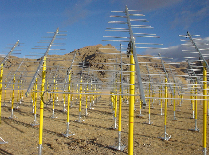
Figure 5: The 21cm Chinese Meter Array (21CMA) in China (http://cosmo.bao.ac.cn/project.html).

experiment	site	type	$\nu$ range	Area	date	goal
			MHz	m2
Mark Ia	Australia	spiral	100-200	few	2007	All Sky
EDGESb	Australia	four-point	100-200	few	2007	All Sky
GMRTc	India	parabola array	150-165	4e4	2007	CSSd
PAPERe	Australia	dipole array	110-190	1e3	2007	PS/CSS/Abs
21CMAf	China	dipole array	70-200	1e4	2007	PS
MWAdg	Australia	aperture array	80-300	1e4	2008	PS/CSS/Abs
LOFARh	Netherlands	aperture array	115-240	1e5	2008	PS/CSS/Abs
SKAi	?	aperture array	100-200	1e6	2015	Imaging

Table 1: HI 21cm Cosmic Reionization Experiments

^ahttp://www.atnf.csiro.au/news/newsletter/jun05/Cosmological_re-ionization.htm
^bhttp://www.haystack.mit.edu/ast/arrays/Edges/index.html
^chttp://gmrt.ncra.tifr.res.in/
^dCSS = cosmic Stromgren Spheres, PS = power spectrum, Abs = absorption
^ehttp://astro.berkeley.edu/$\sim$dbacker/EoR/
^fhttp://cosmo.bao.ac.cn/project.html
^ghttp://www.haystack.mit.edu/ast/arrays/mwa/
^hhttp://www.lofar.org/
ⁱhttp://www.skatelescope.org/

3.4 Pre-reionization signal: the difficulty with probing the ’dark ages’

A number of studies have considered the pre-reionization HI 21cm signal (Loeb & Zaldarriaga 2004; Cen 2006; Barkana & Loeb 2005b; Shethi 2005). The HI 21cm measurements can explore this physical regime at $z\sim 50$ to 300, or redshifts $z>30$. At these frequencies, going to the moon becomes more imperative, due to the rapidly increasing ionospheric opacity and phase effects.

In this redshift regime the HI generally follows linear density fluctuations, and hence the experiments are as clean as CMB studies, and $T_{K}<T_{CMB}$, so a relatively strong absorption signal might be expected. Also, Silk damping, or photon diffusion, erases structures on scales $\ell>2000$ in the CMB at recombination, corresponding to comoving scales = 22 Mpc, leaving the 21cm studies as the only current method capable of probing to very large $\ell$ in the linear regime. The predicted rms brightness temperature fluctuations are 1 to 10 mK on scales $\ell=10^{3}$ to 10⁶ (0.2^o to 1^′′). These observations could provide the best test of non-Gaussianity of density fluctuations, and constrain the running power law index of mass fluctutions to large $\ell$, providing important tests of inflationary structure formation. Sethi (2005) also suggests that a large global signal, up to -0.05 K, might be expected for this redshift range.

The difficulty in this case is one of sensitivity. The sky temperature is $>10^{4}$K, and using the equations in section 3.2, it is easy to show that, even if structures as bright at 10mK on scales of a few arcminutes exist, it would require $\sim 10$ square kilometers of collecting area to detect them. For the more typical small scale structure being considered (ie. $\sim 10"$), the required collecting area increases to $3.6\times 10^{10}$ m². The dynamic range requirements also become extreme, $>10^{8}$. It should also be kept in mind that the sky becomes highly scattered due to propagation through interstellar and interplanetary plasma, with source sizes obeying: $\rm\theta_{min}\sim 1({{\nu}\over{1MHz}})^{-2}$deg. Hence the all objects in the sky are smeared to $>4"$ for frequencies $<30$ MHz.

4 Very low frequency science (1 MHz to 10MHz) from the moon

A new astronomical window is opened up by going outside the Earth’s ionosphere, between 1 MHz and 10MHz. The lower limit of 0.1 MHz is set by a combination of the heliospheric plasma frequency, and Galactic free-free absorption. We briefly discuss some interesting science opportunities generated by opening up this window (see Burns this volume). This is clearly an incompletely list, and a key point is that the most interesting discoveries that come from opening a new astronomical window are usually not predictable.

• Coronal mass ejections (CME’s) and space weather: Solar magnetic activity generates ionized mass ejections which can severely affect satellites, and other electronic equiptment, eg. associated with a lunar base. These CME’s can be studied at low radio frequencies (Bastian 2006), both passively through various plasma radiation processes, and through remote sensing (radar). A low frequency radio telescope could play an important role as part of a severe space weather ’early warning system’, allowing for appropriate action to be taken for satellite and lunar base safety.

• Planetary radio emission: Bursts of low frequency emission from Jupiter were discovered early-on by Franklin & Burke (1956), associated with the interaction between the Io-driven ion torus and Jupiter’s magnetic field. Many other low frequency emission mechanisms exist for planets, ranging from aurural emission associated with the interaction of the solar wind and planetary magnetic fields, to lightening in planetary atmostpheres (Woan et al. 1997).

• Extrasolar planetary radio bursts: Lazio et al. (2004) has calculated the expected frequency and signal strength of Jupiter-burst type radio emission from all extrasolar planets known at the time, based on a coarse relationship between planet mass and radio power (Figure 6). A low frequency radio telescope has the potential to be an effective planet-finding instrument through low frequency radio bursts at the mJy level between 1 and 100 MHz.

• Neutrino interactions with the lunar regolith: High energy neutrinos passing through the lunar regolith (from the far side), may interact with the regolith, generating a shower of energetic particles which emit a burst of beamed Cherenkov radiation. Attempts have been made to use the moon as a neutrino detector through the resultant low frequency radio emission (Hankins et al. 2000). A set of local detectors on the moon could be used to study the emission in situ (Falcke 2006).

• Synchrotron emission by intergalactic collisionless shocks: The shocks produced by converging flows in the intergalactic medium accelerate a power-law tail of electrons to relativistic energies. The synchrotron emission by these electrons in the post-shock magnetic fields paints a cosmic web of radio emission and should be brightest at low frequencies (Keshet et al. 2005). The emission is already seen in the accretion shocks around X-ray clusters (Bagchi et al. 2006).

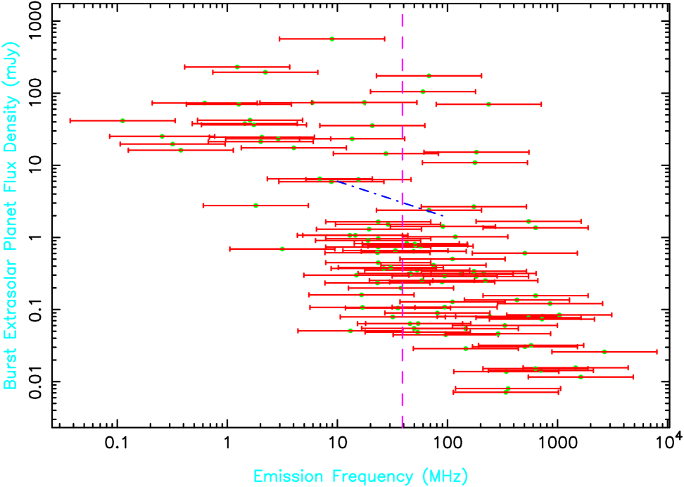
Figure 6: Predicted radio burst flux densities from all known extrasolar planets (Lazio et al. 2004), with approximate indication of the sensitivity (blue dash-dot line) of a ground-based, long-wavelength telescope like the Long Wavelength Array (Kassim et al. 2006), assuming a 15 minute integration.

5 Near-term lunar investigations

There are a number of issues that could be investigated in preparation for a lunar implementation of a low frequency radio telescope.

• Lunar ionosphere: Studies in the 1970’s using the LUNA lunar orbiters, suggested that the moon may have a significant ionosphere, with a day side plasma frequency of about 1MHz and a night side value of 0.2 MHz (Vyshlov 1974). The origin, or even existence, of this ionosphere remains unclear (Bauer 1976), with possible sources being radioactivity on the moon, capture of the solar wind, and ionization by cosmic rays. Even if real, the plasma frequency is still at least an order of magnitude below the Earth’s value, hence opacity is not an issue. However, the issue of electronic path-length variations due to the lunar ionosphere needs to be explored. Experiments are needed to test the existence of the lunar ionosphere, and if real, determine if there are significant electronic path-length variations at frequencies $<200$ MHz.

• Computing requirements and power consumption: We discussed in section 3.3 that the data rates for a full-up array to study reionization are extreme (1.6 Tb/s). The station data cannot be transmitted directly to Earth, but need to correlated on the moon. The power consumption is significant, eg. the Blue Gene correlator for LOFAR draws 0.15MW of power. This raises the potential requirement of low power supercomputing, and early design studies are required to address this issue. Of course, for an initial small test array, the data rate may be managable, eg. 8 elements with 200 MHz/8 bit sampling implies a data rate of only 12.8 Gbit s^-1. On the timescales being considered ($\sim 2020$), Moore’s law for computing should also provide significantly more capabilities than are currently available.

• RFI shielding: Given the power requirements above, it has been proposed to locate the array in a crater near the lunar pole (Heidemann 2000; Woan et al 1997). Within the crater there can be a region of permanent shadowing from the Earth, and yet on the crater’s rim there may be eternal sunlight. The question arises: how far around the limb of the moon does the array have to be for adequate shielding from terrestrial radio emission?

• Current arrays: The current arrays will be key path-finders in the study of element design, array design, foreground removal, wide-field imaging with large fraction bandwidths, correlation of many element interferometers, and related. These arrays will also demonstrate whether the requisit very high dynamic range images ($\sim 10^{6}$) can be generated in the presence of large ionospheric phase distortions and strong terrestrial interference. If not, then the far side of the moon becomes imperative for future probes of this key epoch of cosmic evolution.

• Form a lunar radio telescope working group, to help coordinate near-term studies related to a future lunar radio array, and provide funding for preliminary studies related to a lunar radio telescopes.

• Enforce ITU agreement 22.22, keeping the lunar far-side a radio quiet zone.

6 Summary

Cosmic reionization is the next frontier in observational cosmology. The HI 21cm signal at low frequencies from the neutral IGM during reionization is the most direct probe of the physical processes involved in reionization. A number of low frequency, ground-based path-finder arrays are being planned to make the first detection of the neutral IGM during reionization. The far-side of the moon presents the unique opportunities of being outside the Earth’s ionosphere, and shielded from terrestrial interference.

Beyond supporting the current ground-based efforts, we have proposed a number of design, environment, or technical studies that could be performed to pave the way to a lunar low frequency radio telescope. Lunar development could be staged, while providing results of scientific interest along the way. A simple experiment would be a single low frequency dipole to study the all-sky reionization signal. The next phases could involve arrays of similar aperture to the current ground-based arrays, to study the statistical signal, and other aspects, like absorption toward very high $z$ radio sources. The final stage could entail a full square kilometer of collecting area to perform 3D tomographic imaging of the neutral intergalactic medium during cosmic reionization. We should point out that the Europeans are well along in planning for the first automated low frequency radio telescope on the moon, with a planned Ariane V launch sometime in the coming decade.