Polarization diagnostics of proton beams
in solar flares

Abstract

We review the problem of proton beam bombardment of solar chromosphere considering the self-consistent NLTE polarized radiation transfer in hydrogen lines. Several observations indicate a linear polarization of the H$\alpha$ line of the order of 5% or higher and preferentially in radial direction. This polarization is often explained as anisotropic collisional excitation of the $n=3$ level by vertical proton beams. Our calculations indicate that deceleration of the proton beam with initial power-law energy distribution together with increased electron and proton densities in the H$\alpha$ forming layers lead to a negligible line polarization. Thus the proton beams seem not to be a good candidate for explanation of the observed polarization degree. On the other hand, the effect of electric return currents could perhaps provide a better explanation of the observed linear polarization. We report the new calculations of this effect.

1 Introduction

There is an observational evidence for the fast electron beams (10–100 keV) and also for the fast proton beams ($\sim 10$ MeV) bombarding the solar chromosphere during the impulsive and gradual phase of solar flares (Korchak 1967; Orrall & Zirker 1976). This bombardment is consistent with the “standard model” of solar flare which assumes an injection of the high energetic particles from a coronal reconnection site to the chromosphere. It results in heating and nonthermal excitation of the chromospheric gas. The standard semiempirical models of the flaring chromosphere (Machado et al. 1980) are based on the series of continuum and lines observations and do not take into account a nonthermal excitation; they rather overestimates the chromospheric temperature to explain an increased radiative emission.

Also the low energy proton beams (below 1 MeV) could play a significant role in the flare physics but their presence in the chromospheric layers is still uncertain due to their negligible bremsstrahlung radiation. There are however different ways how to diagnose them. For instance:

1. Ly$\alpha$ red wing emission due to charge exchange effect (Canfield & Chang 1985; Zhao et al. 1998).

2. Modification of the lines intensity profiles due to nonthermal excitation (Hénoux et al. 1993; Xu et al. 2005a).

3. Detection of a linear polarization of the lines due to an anisotropic collisional excitation (i.e. impact atomic polarization).

Moreover, several unanswered questions still remain about the electron beams. Especially the physics of the return currents creation and their influence on lines formation.

Measurement of linear polarization in solar flares is a complicated task due to the high spatial and time gradients. Lot of observations report the polarization degree of H$\alpha$ of the order of few percent (Hénoux & Chambe 1990; Vogt & Hénoux 1999; Hanaoka 2003; Xu et al. 2005b). Direction of this polarization is usually found to be either radial or tangential with respect to the limb and its degree is up to 5% or even exceeds 10% in the few cases. The standard interpretation of these measurements is anisotropic excitation by proton and/or electron beams. By contrast, no measurable linear polarization above the noise level at 0.1% was found in the set of many different flares by another authors (Bianda et al. 2003, 2005).

Our objective is to find out if the measurements of a linear polarization degree of the hydrogen H$\alpha$ line are a promising tool for the diagnostics of the low-energy proton beams. Moreover, we present a first quantitative estimation of the polarizing effect of the return electric currents taking properly into account depolarizing collisions and radiative transfer.

We start with the standard semiempirical model of the flaring atmosphere F1 (Machado et al. 1980) with a fixed temperature structure. We include the nonthermal collisional rates of excitation and ionization to obtain the new line profiles. We use a stationary modeling of the polarized radiation transfer in the chromospheric hydrogen lines using a multilevel NLTE polarized transfer code.

2 H$\alpha$ impact polarization

Let us assume a beam of the unidirectional charged colliders and let their energy be high enough to excite the $n=3$ level (i.e. higher than 12.1 eV). In fact, the $n=3$ level is composed of five quasi-degenerated fine structure levels. Some of them can be polarized, hence the photons emitted in the H$\alpha$ (and Ly$\beta$) line are in general polarized. An anisotropical excitation of these levels by either protons or electrons is one of the processes which can lead to polarization of these levels. The orientation of electric vector of this radiation can be either parallel or perpendicular to the velocity of the beam (cf. Figure 1). A beam is expected to follow the direction of magnetic field which is assumed to be vertical in the atmosphere; hence the linear polarization is either radial or tangential with respect to the solar limb.

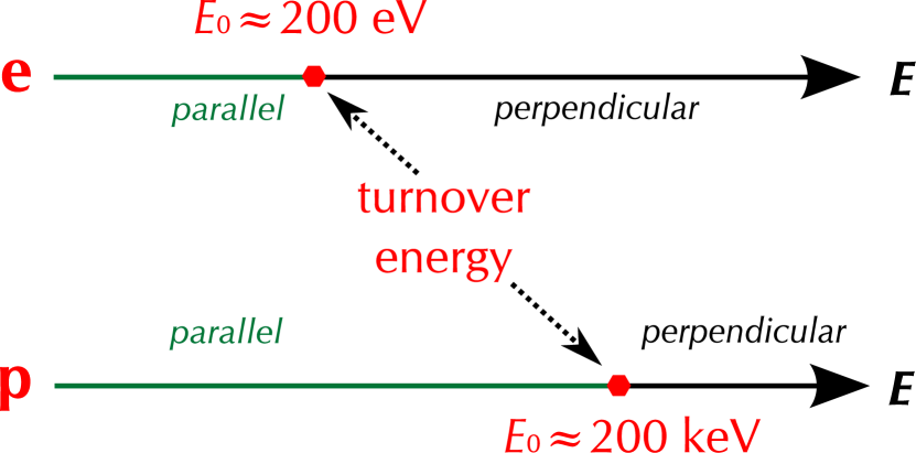
Figure 1: Linear polarization of the photons emitted in the H$\alpha$ line perpendicularly to the collisional trajectory (i.e. in the direction of a maximum polarization degree). For both the electrons and protons impacts, low energies of collisions lead to linear polarization of the emitted photons in the direction parallel to the collisional trajectory. A polarization direction above the so-called turnover energy is perpendicular to it.

The assumptions above should lead to an upper theoretical limit for the H$\alpha$ linear polarization. The coordinate system definition is given in Figure 2. In such a reference frame, only the Stokes parameters $I$ and $Q$ are in general nonzero.

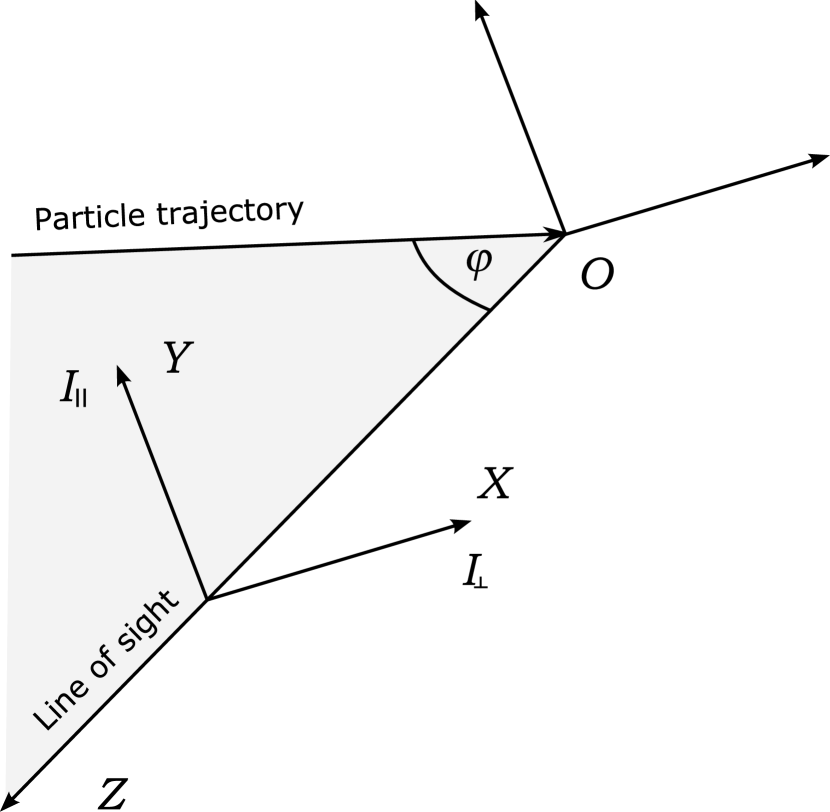
Figure 2: We use a right-handed coordinate system with $Y$-axis in the collisional plane and $Z$-axis in the line of sight direction. Due to cylindrical symmetry of the model, only Stokes parameters $I$ and $Q$ do not generally vanish in this coordinate system.

We are interested especially in a modeling of the radial polarization. It follows from Figure 1 that this orientation is associated with the low-energy electrons or the low-energy protons moving vertically in the atmosphere.

3 Formalism and methods

A vertical magnetic field is assumed to be of the strength of few hundreds gauss (Vogt et al. 1997). It can be shown that in this regime and in the plasma conditions under consideration (see below) fine structure splitting of the hydrogen levels up to $n=3$ is a good approximation (Sahal-Bréchot et al. 1996). The hyperfine splitting of the levels can be neglected because it does not significantly affect a linear polarization degree (Bommier et al. 1986a). In addition, a lifetime of the fine structure levels is reduced by collisions with the background protons and electrons and thus the hyperfine levels of the excited states completely overlap. To describe an atomic state we adopt the formalism of the atomic density matrix in the basis of irreducible tensorial operators $\rho^{K}_{Q}(nlj)$ (Fano 1957), with the traditional meaning of the symbols. We neglect all the quantum coherences between different fine structure levels due to their large separation in comparison to their width and due to the selection rules for the optical transitions. A magnetic field is able to destroy all the quantum coherences between the Zeeman sublevels of any level. In the formalism of irreducible tensors it means that all the multipole components of $\rho$ with $Q\neq 0$ are identically zero, $\rho^{K}_{Q}(nlj)=\delta_{Q0}\rho^{K}_{Q}(nlj)$. On the other hand, the strength of a magnetic field is not so high to induce a Zeeman splitting large enough to lead to the complicated level-crossing effects. Finally, because of the assumption of absence of any circularly polarized radiation, the odd ranks $K$ of the density matrix are identically zero. All these assumptions lead to the simplifications of the formalism.

The results of our modeling are strongly dependent on the collisional cross-sections of the different excitation and ionization transitions. We consider the following collisional processes and cross-sections data:

• Excitation and charge exchange for a proton beam using the close-coupling cross-sections data of Balança & Feautrier (1998).

• The dipolar transitions between the fine structure levels $nlj\to nl\pm 1j^{\prime}$ for interaction with the background electrons, protons, and the beam are calculated using the semiclassical theory of Sahal-Bréchot et al. (1996).

• Excitation of the levels populations by the background electrons (the cross-sections data are taken from the AMDIS database, http://www-amdis.iaea.org).

For the purposes of impact polarization studies it is necessary to calculate all the collisional transition rates

$$C^{K\to K^{\prime}}_{nlj\to n^{\prime}l^{\prime}j^{\prime}}=N_{\rm P}\int{\rm d}^{3}\vec{v}f(\vec{v})v\sigma^{K\to K^{\prime}}_{nlj\to n^{\prime}l^{\prime}j^{\prime}}(\vec{v})\;,$$ (1)

for transitions $\rho^{K}_{0}(nlj)\to\rho^{K^{\prime}}_{0}(n^{\prime}l^{\prime}j^{\prime})$. These rates enter the equations of statistical equilibrium together with the radiative rates $R^{K\to K^{\prime}}_{nlj\to n^{\prime}l^{\prime}j^{\prime}}$ in the so-called impact approximation (Landi Degl’Innocenti 1984; Bommier & Sahal-Bréchot 1991). The equations of statistical equilibrium have the form

$$\sum_{nljK}(C^{K\to K^{\prime}}_{nlj\to n^{\prime}l^{\prime}j^{\prime}}+R^{K\to K^{\prime}}_{nlj\to n^{\prime}l^{\prime}j^{\prime}})\rho^{K}_{0}(nlj)=0\;.$$ (2)

To take properly into account a coupling of the atomic states at the different atmospheric points, it is necessary to solve a system of equations (2) coupled by the radiative transfer equation for Stokes vector $\vec{I}=(I,Q)^{\rm T}$. Its evolution along the path $s$ is given by

$$\frac{{\rm d}\vec{I}}{{\rm d}s}=\vec{J}-\vec{K}\,\vec{I}\;.$$ (3)

In this equation, $\vec{J}$ is the emissivity vector and $\vec{K}$ is the so-called propagation matrix. We use our multigrid code (Štěpán 2006) to solve this problem in the plan-parallel geometry, out of the LTE approximation (the case of the chromospheric H$\alpha$ line).

4 Results for the proton beams

The temperature structure of the atmosphere is fixed and given by the F1 model. A new ionization degree and the atomic states along the chromosphere are obtained by solution of the system of the Eqs. (2) and (3).

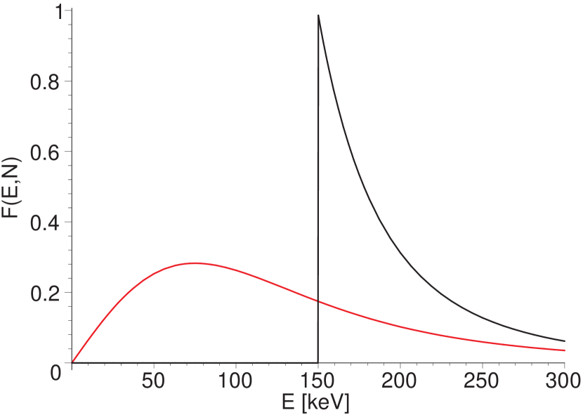
Figure 3: Energy distribution of a beam flux (in arbitrary units), $\delta=4$, $E_{\rm c}=150~{}{\rm keV}$. The initial sharp-peaked power-law energy distribution (upper curve) becomes flatter in the region where the slowest protons are stopped (lower curve).

The initial energy distribution of the proton beam at the top of the chromosphere is (as usually) expected to be given by the power-law

$$F(E)\sim E^{-\delta}\;,\qquad E>E_{\rm c}\;,$$

with the lower energy cut-off $E_{\rm c}$ and the spectral index $\delta$. After crossing some column depth, the distribution is modified by collisions with various atmospheric species (see Figure 3), (Emslie 1978; Canfield & Chang 1985). The protons most efficient in creation of the $n=3$ level polarization have a small energy about $5~{}{\rm keV}$ (Balança & Feautrier 1998). A number of such protons in the region of the H$\alpha$ line core formation is very small compared to the number of protons of an energy about $E_{\rm c}$ at the injection site (cf. Vogt et al. 1997, 2001). As a result, there is only a small number of low-energy protons even for the high initial beam fluxes.

The electron (proton) densities of the chromosphere obtained as a result of the NLTE calculations are of the order of $10^{12}~{}{\rm cm^{-3}}$ in the regions of the H$\alpha$ centre and near wings formation (Figure 4). These densities were computed using the code of Kašparová & Heinzel (2002) adapted for the proton beams studies.

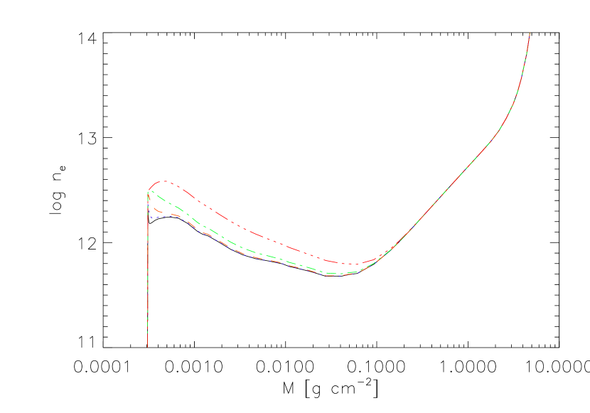
Figure 4: Electron density for the model F1. The plot corresponds to the case of $\delta=4$, $E_{\rm c}=150\;{\rm keV}$. Thermal case is plotted by a solid line, the non-thermal beam fluxes are $\mathcal{E}_{0}=10^{8}$ (dot), $10^{9}$ (dash), $10^{10}$ (dash-dot), and $10^{11}\,{\rm erg\,cm^{-2}\,s^{-1}}$ (dash-dots).

It was shown by Bommier et al. (1986b) that depolarization of the hydrogen levels by collisions with the background electrons and protons becomes important even at the densities of the order of $10^{10}~{}{\rm cm^{-3}}$. It is therefore expected that the depolarization effect will play a crucial role in the chromospheric conditions.

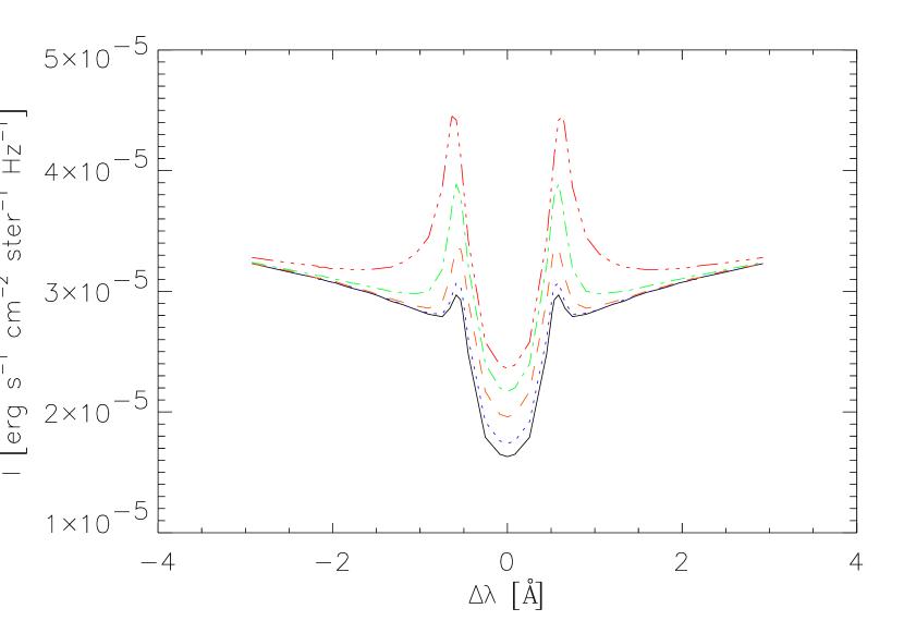
Figure 5: H$\alpha$ line intensity profiles for the same set of models as in the Figure 4.

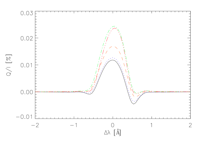
Figure 6: Emergent fractional linear polarization $Q/I$ profiles (%) computed close to the limb ($\mu=0.11$) for the same set of models as in the Figure 4. A positive sign of $Q/I$ means the tangential direction of polarization, while a negative sign is the radial one.

The theoretical line profiles calculated for a set of the proton beam energy fluxes are plotted in the Figures 5 and 6. As it can be seen in Figure 6, a polarization degree of the emergent H$\alpha$ line close to the limb is extremely small. Moreover, its orientation is tangential and not radial as it was expected for the low-energy proton impacts. This polarization is mainly due to resonance scattering of the radiation, while the impact polarization effect is not seen. The degree of 0.02% is well below any measurable value to day.

5 Effect of electronic return currents

It seems that linear polarization of the H$\alpha$ line due to slow proton beams is not a good diagnostics tool even if very restrictive conditions on the beam anisotropy are postulated. Another phenomena which could explain the observed radial polarization are the return currents (RC) associated with the electron beams. The detailed studies of the collective plasma processes show that the return currents which neutralize a huge electric current of the beam can be formed if several plasma conditions in the atmosphere are fulfilled (Norman & Smith 1978). The atomic excitations caused by the return current were shown to be more important than the effect of the beam itself in some depths (Karlický et al. 2004).

Karlický & Hénoux (2002) propose the anisotropical impacts of the slow (few deca-eV) RC as an explanation for the observed linear polarization of the H$\alpha$ line. However, all these calculations neglected the effects of depolarizing collisions and polarized radiative transfer. We have studied a simple model of monoenergetic electron beam with the initial energy flux of $1.2\times 10^{12}~{}{\rm erg\;cm^{-2}\;s^{-1}}$ composed of the electrons with the energy 10 keV penetrating the F1 atmosphere. The electron-hydrogen cross-sections for the dipolar transitions have been calculated by the semiclassical method with momentum transfer (Bommier 2006). These calculations show that return current is locally able to produce a significant atomic polarization, but it is decreased by the depolarizing collisions and high intensity of radiation. If all these effects are taken into account together with radiation transfer, the emergent linear polarization degree in the centre of H$\alpha$ is only about 0.25% in the radial direction. That is still one order of magnitude below the measured values.

6 Conclusions

A net impact polarization of an electron beam + RC seems to be a more promising explanation of the observed linear polarization than the proton beam impacts. However, collisional depolarization by background electrons and protons together with the increased radiation intensity can destroy most of the impact atomic polarization.

Several things have been simplified to make our models traceable:

1. The semiempirical model F1 overestimates the atmosphereric temperature. As a result, depolarization and lines intensities are also overestimated.

2. No time dependence was considered. Detailed time-dependent modeling could possibly explain some aspects of polarization generation.

3. The plane-parallel model has a limited applicability and more complex geometry could be considered to interpret the observations.

4. If a RC is carried by a substantial number of background electrons, they do not contribute to the collisional depolarization in the same way as the thermal electrons. That was not taken fully into account in our models.

5. The beams are never purely directional and vertical and their scattering may lead to further decrease of the impact polarization. The monoenergetic electron beam + RC is not a satisfactory physical model.

A quantitative estimation of all these effects should be a subject of the future studies.

References

- Balança & Feautrier (1998) Balança, C. & Feautrier, N. 1998, A&A, 334, 1136
- Bianda et al. (2005) Bianda, M., Benz, A. O., Stenflo, J. O., Küveler, G., & Ramelli, R. 2005, A&A, 434, 1183
- Bianda et al. (2003) Bianda, M., Stenflo, J. O., Gandorfer, A., Gisler, D., & Küveler, G. 2003, in Astronomical Society of the Pacific Conference Series, ed. J. Trujillo-Bueno & J. Sanchez Almeida, Vol. 307, 487
- Bommier (2006) Bommier, V. 2006, in proceedings of the 4th Solar Polarization Workshop, ed. R. Casini (ASP Conf. Series, in press)
- Bommier et al. (1986a) Bommier, V., Leroy, J. L., & Sahal-Bréchot, S. 1986a, A&A, 156, 79
- Bommier et al. (1986b) Bommier, V., Leroy, J. L., & Sahal-Bréchot, S. 1986b, A&A, 156, 90
- Bommier & Sahal-Bréchot (1991) Bommier, V. & Sahal-Bréchot, S. 1991, Ann. Phys. Fr., 16, 555
- Canfield & Chang (1985) Canfield, R. C. & Chang, C.-R. 1985, ApJ, 295, 275
- Emslie (1978) Emslie, A. G. 1978, ApJ, 224, 241
- Fano (1957) Fano, U. 1957, Rev. Mod. Phys., 29, 74
- Hanaoka (2003) Hanaoka, Y. 2003, ApJ, 596, 1347
- Hénoux & Chambe (1990) Hénoux, J.-C. & Chambe, G. 1990, Journal of Quantitative Spectroscopy and Radiative Transfer, 44, 193
- Hénoux et al. (1993) Hénoux, J.-C., Fang, C., & Gan, W. Q. 1993, A&A, 274, 923
- Karlický & Hénoux (2002) Karlický, M. & Hénoux, J.-C. 2002, A&A, 383, 713
- Karlický et al. (2004) Karlický, M., Kašparová, J., & Heinzel, P. 2004, A&A, 416, L13
- Kašparová & Heinzel (2002) Kašparová, J. & Heinzel, P. 2002, A&A, 382, 688
- Korchak (1967) Korchak, A. A. 1967, Soviet Astronomy, 11, 258
- Landi Degl’Innocenti (1984) Landi Degl’Innocenti, E. 1984, Sol. Phys., 91, 1
- Machado et al. (1980) Machado, M. E., Avrett, E. H., Vernazza, J. E., & Noyes, R. W. 1980, ApJ, 242, 336
- Norman & Smith (1978) Norman, C. A. & Smith, R. A. 1978, A&A, 68, 145
- Orrall & Zirker (1976) Orrall, F. Q. & Zirker, J. B. 1976, ApJ, 208, 618
- Sahal-Bréchot et al. (1996) Sahal-Bréchot, S., Vogt, E., Thoraval, S., & Diedhiou, I. 1996, A&A, 309, 317
- Štěpán (2006) Štěpán, J. 2006, in proceedings of the 4th Solar Polarization Workshop, ed. R. Casini (ASP Conf. Series, in press (astro-ph/0611112))
- Vogt & Hénoux (1999) Vogt, E. & Hénoux, J.-C. 1999, A&A, 349, 283
- Vogt et al. (2001) Vogt, E., Sahal-Bréchot, S., & Bommier, V. 2001, A&A, 374, 1127
- Vogt et al. (1997) Vogt, E., Sahal-Bréchot, S., & Hénoux, J.-C. 1997, A&A, 324, 1211
- Xu et al. (2005a) Xu, Z., Fang, C., & Gan, W.-Q. 2005a, Chinese Journal of Astronomy and Astrophysics, 5, 519
- Xu et al. (2005b) Xu, Z., Hénoux, J.-C., Chambe, G., Karlický, M., & Fang, C. 2005b, ApJ, 631, 618
- Zhao et al. (1998) Zhao, X., Fang, C., & Hénoux, J.-C. 1998, A&A, 330, 351