Optimizing Baryon Acoustic Oscillation Surveys –
I: Testing the concordance $\Lambda$CDM cosmology

Abstract

We optimize the design of future spectroscopic redshift surveys for constraining the dark energy via precision measurements of the baryon acoustic oscillations (BAO), with particular emphasis on the design of the Wide-Field Multi-Object Spectrograph (WFMOS). We develop a model that predicts the number density of possible target galaxies as a function of exposure time and redshift. We use this number counts model together with fitting formulae for the accuracy of the BAO measurements to determine the effectiveness of different surveys and instrument designs. We search through the available survey parameter space to find the optimal survey with respect to the dark energy equation-of-state parameters according to the Dark Energy Task Force Figure-of-Merit, including predictions of future measurements from the Planck satellite. We optimize the survey to test the $\Lambda$CDM model, assuming that galaxies are pre-selected using photometric redshifts to have a constant number density with redshift, and using a non-linear cut-off for the matter power spectrum that evolves with redshift. We find that line-emission galaxies are strongly preferred as targets over continuum emission galaxies. The optimal survey covers a redshift range $0.8<z<1.4$, over the widest possible area (6000 sq. degs from 1500 hours observing time). The most efficient number of fibres for the spectrograph is 2,000, and the survey performance continues to improve with the addition of extra fibres until a plateau is reached at 10,000 fibres. The optimal point in the survey parameter space is not highly peaked and is not significantly affected by including constraints from upcoming supernovae surveys and other BAO experiments.

1 Introduction

The most exciting cosmological discovery in recent years has been the observed late–time acceleration of the expansion of the Universe (Riess et al. 1998; Perlmutter et al. 1999). When this observation is combined with other cosmological data from the Cosmic Microwave Background (CMB) and galaxy redshift surveys, the best fit model to all these data is a flat Universe with $\simeq 30$% of its energy density in the form of dark matter and $\simeq 70$% in the form of “dark energy”; a mysterious component of the Universe with an effective negative pressure.

The simplest explanation for dark energy is a “cosmological constant” ($\Lambda$) as introduced by Einstein in his General Theory of Relativity to create a static Universe. In recent times, the cosmological constant has been interpreted as the “vacuum energy”, but the observed value of $\Lambda$ is a factor of $\sim 10^{120}$ smaller than its natural value from particle physics (Krauss & Turner 1995; Carroll 2001). Alternatives to the cosmological constant include time–evolving dark energy models, such as quintessence (Ratra & Peebles 1988; Wetterich 1988), and modifications of gravity at large scales (Deffayet, Dvali & Gabadadze 2002; Carloni et al. 2005; Damour, Kogan & Papazoglou 2002). The current cosmological data is only good enough to measure the local value of the dark energy density. Therefore, the present data prefers a cosmological constant, mainly because it is the simplest model, whilst time–evolving models of dark energy (which possess more free parameters) remain relatively unconstrained by present datasets (see Corasaniti et al. 2004; Bassett et al. 2004; Liddle et al. 2006).

Over the next decade, numerous experiments are proposed, over a wide range of redshifts, to explore the time–evolution of dark energy and determine its density as a function of cosmic time. These experiments (both ground–based and space–based) represent an investment of billions of dollars and essentially use two general techniques to probe the dark energy: geometrical tests of the expansion history of the Universe using “standard tracers” (see below), and/or observations of the rate of growth of large–scale structures (clusters & superclusters) in the Universe. The relative merits of these two techniques, and the proposed experiments, have been explored in detail by the U.S. Dark Energy Task Force (DETF; Albrecht et al. 2006) and a similar endeavour in the U.K.

In this paper, we focus on measurements of the time–evolution of dark energy using observations of the baryon acoustic oscillations (BAOs) from large galaxy surveys. The BAOs are generated by acoustic waves in the baryon–photon plasma in the early Universe, which become frozen into the CMB radiation, and the distribution of matter, soon after the Universe cools and re–combines at $z\simeq 1100$. Over the last 5 years, the scale of these BAOs has been accurately measured in the CMB by a number of experiments (WMAP, Archeops & BOOMERanG), as well as discovered in the distribution of matter (galaxies and clusters) at low redshift (see Miller, Nichol & Batuski 2001; Eisenstein et al. 2005; Cole et al. 2005; Padmanabhan et al. 2006). For example, Eisenstein et al. (2005) used these observations to constrain the flatness of the Universe to 1%, under the assumption that dark energy is a cosmological constant.

As the scale of the BAOs can be predicted to sub–percent accuracy (see Eisenstein, Seo & White 2006; Eisenstein & White 2004), they provide an excellent “standard ruler” which can be used to map the geometry of the Universe through the angular-diameter distance and the Hubble parameter relation (see Blake & Glazebrook 2003; Seo & Eisenstein 2003; Hu & Haiman 2003). Several spectroscopic experiments have been proposed to observe and measure this standard ruler at high redshift and thus constrain the time–evolution of dark energy, e.g., WFMOS (Bassett, Nichol & Eisenstein 2005; Glazebrook et al. 2005a), Baryon Oscillation Probe (Glazebrook et al. 2005b), VIRUS (Hill et al. 2005) in the optical and NIR, and the Hubble Sphere Hydrogen Survey (Peterson et al. 2006) and Square Kilometre Array (Blake et al. 2004) in the radio. These new experiments share the desire to measure millions of galaxy redshifts (at high redshift) over large volumes of the Universe to control the errors from both cosmic variance and Poisson noise (Blake & Glazebrook 2003; Glazebrook & Blake 2005).

Given the large investment in time and money for these next generation BAO experiments, we study here the optimal survey strategy for galaxy redshift surveys like those proposed for WFMOS (Wide-Field Multi-Object Spectrograph; see Glazebrook et al. 2005a). This work builds upon our previous development of the Integrated Parameter Survey Optimization (IPSO) framework (Bassett 2005; Bassett, Parkinson & Nichol 2005) and addresses key observational issues such as:

• What are the optimal redshifts for BAO observations?

• What is the best combination of areal coverage and target density?

• What type of galaxies are the best targets?

Although our answers for these questions are derived for WFMOS–like galaxy surveys, we believe that our results are general to BAO experiments in optical wavebands. The analysis presented in this paper optimises $\Lambda$–cosmologies (i.e., a cosmological constant) for the underlying cosmological model against which we are optimizing. Ideally we would like to optimize the observations for a variety of dark energy models, and we will present such an analysis in a future paper. As a consequence therefore, our conclusions and results naturally favour lower-redshift BAO observations where the effect of $\Lambda$ on the expansion history of the Universe is greatest. We also neglect the improvements to the distance measurements that will arise by reconstructing the acoustic peak in the non-linear regime (see Eisenstein et al 2006b), assuming instead a non-linear cut-off for the power spectrum that evolves with redshift.

In Section 2, we outline our methodology and define the Figure-of-Merit (FoM) used to judge the optimality of different survey designs. In Section 3, we lay out the procedures used to conducting the optimization, while in Section 4, we describe the model we used to determine the density of target galaxies. We present and discuss our results in Sections 5 and 6 respectively. We conclude in Section 7.

2 Optimizing Method

We perform our optimization using the IPSO framework (Bassett 2005). Consider a set of allowed survey geometries, indexed by $s$. For each survey geometry, $s$, we compute an appropriate Figure-of-Merit (FoM) - also known as the utility in Bayesian evidence design, risk or fitness - and optimization then simply proceeds by selecting the survey geometry which extremises (minimising or maximising where appropriate) the FoM. Performing such an optimization therefore requires three elements: a survey configuration parameter space $S$ to search through, a target parameter space $\Theta$ of the parameters that we wish to optimally constrain (labelled $\theta_{\mu,\nu...}$), and a numerical Figure-of-Merit (FoM). We consider each of these three elements in turn.

2.1 Survey Parameters

The survey parameters are those parameters which completely describe the survey we wish to test. We start by splitting the survey into two redshift regimes, one at low redshift ($z\simeq 1$) and one at high redshift ($z\simeq 3$), and considering these regimes completely separately. The properties of the survey in each regime are described by a set of parameters: $\tau$ (survey time in that regime), $A$ (survey area in that regime), $n_{bin}$ (number of contiguous redshift bins in that regime), $z_{i}$ (median redshift of the $i$th redshift bin), and $dz_{i}$ (half-width of the $i$th redshift bin). There is also a further parameter, $n_{p}$, which is the number of pointings performed per field–of–view, i.e., the number of times the telescope observes the same patch of the sky. This parameter is derived from the other parameters, using a model of the galaxy number density as a function of exposure time, in conjunction with the assumed number of fibres. All of these parameters are listed in Table 1.

Table 1: Survey parameters in each redshift regime

Survey Parameter	Symbol
Survey time	$\tau_{low}$, $\tau_{high}$
Area covered	$A_{low}$, $A_{high}$
Number of redshift bins	$n_{bin}$
Midpoint of ith redshift bin	$z_{i}$
Half-width of ith redshift bin	$dz_{i}$
Number of pointings	$n_{p}(low)$, $n_{p}(high)$

In selecting a survey, we are also constrained by the technical characteristics of the proposed instrumentation. In this paper, we only consider a WFMOS–like experiment, whose important properties are summarized in Table 2. Firstly, there is the total telescope time available, divided such that $\tau_{\rm Total}=\tau_{high}+\tau_{low}$. There is also the field–of–view of the telescope (FoV), which provides the amount of area that can be observed per telescope pointing, and the number of fibres ($n_{fibres}$), which limits the number of objects that can be observed simultaneously. We include the telescope aperture and fibre diameter of the instrument, even though they are not direct constraint parameters, because they affect the exposure time required to obtain redshifts of galaxies. Note that, whilst this paper is mainly concerned with finding the best survey for a given instrument, we can also compare the performance of different instruments, which we do in section 6.3.

We include an “overhead” period between each observation, which is considered as a period of “dead” time that is added on to the exposure time to get the total time per pointing. We define a pointing to be an exposure period to fill (or attempt to fill) all of the fibres. Even if the telescope is not actually moved between two successive pointings on the sky, the fibres themselves would be re–positioned (with the extra overhead time given in Table 2), and we would count this as two separate pointings. We do not consider optimal tiling algorithms here. Finally, we include limits on the minimum and maximum exposure time per pointing.

We also impose constraints on the redshift regimes. At low redshift, there is no benefit in measuring the BAOs at $z<0.5$ because of the recent measurements by Eisenstein et al. (2005) and Cole et al. (2005). There are also photometric-redshift survey observations of the BAOs at $z\simeq 0.5$ by Padmanabhan et al. (2006). Therefore, we constrain the “low redshift” regime in Table 2 to fall within the range $0.5<z<1.5$. The upper limit derives from the wavelength coverage of the WFMOS spectrographs, beyond which the [OII] emission line and 4000Å  break shift out of the optical window, necessitating infra-red spectographs.

We also consider a “high redshift” regime contained within the limits $2.5<z<3.5$, motivated by observations of Lyman Break and Lyman-$\alpha$ emission galaxies at $z\sim 3$ (Steidel et al. 1999). Spectroscopic redshifts for these galaxies are possible as the Lyman Break and Lyman-$\alpha$ features are redshifted into the optical window.

Table 2: Constraint parameters

Constraint Parameter	Value
Total observing time	1500 hours
FoV	1.5o diameter
$n_{fibres}$	3000
Aperture	8m
Fibre diameter	1 arcsec
Overhead time	10 mins
Minimum exposure time	15 mins
Maximum exposure time	10 hours
Low redshift range	$0.5<z<1.5$
High redshift range	$2.5<z<3.5$

2.2 Target Parameters

The target parameter space $\Theta$ is for our purposes the cosmological parameter space. The measurement of BAOs in the tangential direction will allow us to measure the angular diameter distance to a given redshift bin, whilst measurement of BAOs in the radial direction will allow us to measure the Hubble expansion rate in the redshift bin. The angular-diameter distance (in a flat universe containing only matter and dark energy) is given by,

$$d_{A}(z)=\frac{c}{H_{0}(1+z)}\int_{0}^{z}\frac{dz^{\prime}}{E(z^{\prime})}\,,$$ (1)

where $E(z)$ is the normalised expansion as defined by,

$$E(z^{\prime})=\sqrt{(\Omega_{m}(1+z^{\prime})^{3}+\Omega_{DE}f(z^{\prime}))}\,,$$ (2)

where

$$f(z)=\exp{\int\frac{3(1+w(z))}{1+z}dz}\,,$$ (3)

and $w(z)=p/\rho$ is the equation of state parameter of the dark energy. In a flat universe, $\Omega_{DE}=1-\Omega_{m}$, which leaves only $H_{0}$, $\Omega_{m}$ and $w(z)$ to be measured by any survey of the Universe.

For our optimization, we selected the Linder (Chevallier & Polarski, 2001, Linder, 2003) expansion of $w$ in terms of the scale factor ($a$) of the Universe, rather than redshift, as given by,

$$w(a)=w_{0}+w_{a}(1-a)\,.$$ (4)

We therefore optimize each survey for the values of $w_{0}$ and $w_{a}$, whilst marginalizing over $H_{0}$ and $\Omega_{m}$. For these latter two parameters, we recast them as $\Omega_{m}h^{2}$ and $\Omega_{m}$ (where $h=H_{0}/100$ km s^-1 Mpc^-1).

As discussed in the Introduction, we assume a cosmological constant ($\Lambda$) for the underlying cosmological model when constructing our survey designs. However, we stress here that we still perform the optimization using both the $w_{0}$ and $w_{a}$ parameters as outlined above. This is the correct methodology as a priori we do not know the true cosmological model that describes the Universe and must therefore include the necessary parameters needed to describe the range of models that possibly fit the observations. Furthermore, it will allow us to compare these results to future predictions based on a wider variety of dark energy models. We note the existence of possible extensions to more complicated sets of target parameters, such as those suggested by Albrecht & Bernstein (2006).

2.3 Figure of Merit

The Figure-of-Merit (FoM) is a single real number assigned to each survey configuration tested. The survey with the best FoM is then defined as the optimal survey. The FoM we consider here is defined by (Bassett 2004),

$$FoM(s_{i})=\int_{\bf\Theta}I(s_{i},\vec{\theta})p(\vec{\theta})d\vec{\theta}\,,$$ (5)

where $I(s_{i},\vec{\theta})$ is the performance of a survey configuration ($s_{i}$), given a particular value of the target parameters ($\vec{\theta}$) (here the dark energy parameters), and $p(\vec{\theta})$ is a “weighting vector” that places emphasis on particular volume of the parameter space. By integrating over the entire cosmological parameter space, the FoM we produce is only dependent on the survey configuration.

Although there are many choices for $I(s_{i},\theta)$ (Bassett 2005), we follow Bassett, Parkinson and Nichol (2005) and choose D-optimality as defined by

$$I(s,\theta)=\log\mbox{det}({\bf F}+{\bf P}),$$ (6)

where “det” denotes the matrix determinant and ${\bf P}$ is the prior precision matrix (the Fisher matrix of all the relevant prior data) and ${\bf F}$ is the Fisher information matrix of the predicted likelihood, which we estimate using the method described by Glazebrook & Blake (2005). From this, ${\bf F}+{\bf P}$ is the Fisher matrix of the posterior and $\mbox{det}({\bf F}+{\bf P})$ is inversely proportional to the square of the volume of the posterior ellipsoid. We set ${\bf P}$ to zero, assuming no prior knowledge about the dark energy. Therefore, a larger value for the FoM corresponds to smaller errors on the parameters of interest. More details on how we calculate the Fisher matrix are given in Appendix A.

In the US Dark Energy Task Force report (DETF; Albrecht et al. 2006b), a slightly different Figure-of-Merit is used. Their FoM is defined to be the reciprocal of the area in the $w_{0}$–$w_{a}$ plane that encloses the 95% C.L. region, whereas ours is the reciprocal of the square of the area in the $w_{0}$–$w_{a}$ plane that encloses the 68% region. Therefore our FoM is proportional to the square of the DETF FoM.

3 Optimization Procedure

The computational problem of searching through the survey parameter space ($S$) is that the available volume of this space is very large. Therefore we use a Monte-Carlo Markov Chain (MCMC) procedure (the Metropolis-Hastings algorithm; Metropolis et al. 1953; Hastings 1970) to conduct a random walk through the parameter space to map the survey parameters as a function of FoM, and find the optimal survey and the survey configuration associated with it. As there may be a number of degenerate minima in this parameter space (i.e., surveys with very different configurations but similar FoMs), we also use the simulated annealing algorithm (Kirkpatrick et al. 1983; Cerny 1985) to cool and heat the chains generated by the MCMC process, such that we can be sure we reach (or get very close to) the global maximum.

In MCMC, each new point in the chain is selected as a random point near to the previous point with a probability equal to the ratio of FoMs of the two corresponding surveys, such that a better survey will usually be selected, whilst a worse survey will sometimes be selected. In simulated annealing, the probability is multiplied by an extra factor known as the “temperature”. When the temperature is large, a wide variety of surveys are selected with almost equal probabilities, but as the chains cool, and the temperature goes to zero, the algorithm is weighted towards selecting only better surveys. We cycle the temperature, using some thermodynamic scheduling, to guarantee that we reach the global minimum in this large parameter space. In Figure 1, we show how these MCMC chain with different thermodynamic schedules converge to the true optimal survey configuration (the best FoM) after $\sim 10^{4}$ steps.

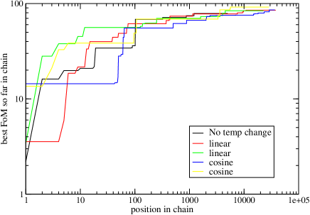
Figure 1: The best Figure-of-Merit found by the MCMC process as a function of position in the chain for different thermodynamic schedules. These chains are taken from the optimization of surveys with two low redshift bins and one high redshift bin.

For this analysis, we judge the effectiveness of each survey in terms of the cosmological constant ($\Lambda$) model and, as such, the weighting function $p(\vec{\theta})$ from Eq. 5 is set to a delta-function around the best-fit $\Lambda$ model,

$$FoM({s_{i}})=\int_{\bf\Theta}I(s_{i},\vec{\theta})\delta(\Lambda)d\vec{\theta}=I(s_{i},\Lambda)=\mbox{det}({\bf F})\,.$$ (7)

The optimization proceeds as follows:

1. Select a test survey configuration ($s$) from the given survey parameters (area coverage, redshift bins, exposure time etc.) from parameter space ($S$).

2. Estimate the number density of galaxies that will be observed by this test survey using luminosity functions described in Section 4.

3. Estimate the error on $d_{A}(z)$ and $H(z)$ using scaling relations given in Blake et al. (2006).

4. Calculate the Fisher matrix of parameters, using distance data plus other information that will be available from future experiments. This takes the form of Gaussian priors on $\Omega_{m}h^{2}$ and $\Omega_{m}$. For $\Omega_{m}h^{2}$ we use predicted Planck measurement with $\mu=0.147$ and $\sigma=0.003$. For $\Omega_{m}$ we assume $\mu=0.3$ and $\sigma=0.01$. The procedure for this is outlined in Appendix A.

5. Use the Fisher matrix to calculate Figure-of-Merit for survey $s$, as given by Eq.7, using the $(w_{0},w_{a})$ submatrix.

6. Repeat steps 1 through 5, conducting a MCMC search over the survey configuration parameter space $S$, attempting to minimize the FoM.

There are a number of assumptions that we make in doing this optimization that may bias the results in some manner. They are: (1) we are applying a constant number density with redshift using photometric-redshift target pre-selection in order to ensure the most efficient use of fibres, (2) we are optimizing for $\Lambda$CDM, and (3) we are neglecting reconstruction of the acoustic peak at non-linear scales (Eisenstein et al 2006b) (i.e. assuming a non-linear power spectrum cut-off which evolves with redshift in the same style as Glazebrook & Blake 2005).

The assumed fiducial cosmological parameters are $\Omega_{m}=0.3$, $H_{0}=70{\rm kms^{-1}Mpc^{-1}}$, $\Omega_{m}h^{2}=0.147$, and of course $w_{0}=-1$ and $w_{a}=0$. We also assume a baryon fraction of 0.15, giving $\Omega_{b}=0.045$ and a sound horizon of $s=108h^{-1}{\rm Mpc}$.

When optimizing a system, it is important to know how sensitive the optimal solution is to a slight change in the parameters. We quantify this sensitivity using “flexibility bounds”, which are defined as the change in a survey parameter which decreases the FoM by 20% relative to the optimum. The value of 20% is arbitrary, based on comparisons of survey performance with other planned experiments and possibilities of theoretical advancements. What this will mean for the error bars on the two parameters ($w_{0}$, $w_{a}$) is that, since the FoM is the square of the 1-$\sigma$ error ellipse, a 20% decrease in the FoM corresponds to a 10% increase in the size of the error ellipse, or a $\approx 5\%$ increase in each error bar. We computed the flexibility bounds by considering the effects of changing only one parameter, whilst keeping the other parameters at their optimal values (we do not account for correlations between parameters in their FoM dependence).

4 Galaxy number counts modelling

We describe here our model for converting a survey exposure time and redshift range into an observed number density of target galaxies for spectroscopy. The number counts calculator is constructed using the observed properties of $z\sim 1$ and $z\sim 3$ galaxies taken from the literature (e.g. observed luminosity functions and distributions of equivalent widths of emission lines). We do not attempt to model observational issues such as the reliability of redshift extraction or confusion in line identifications.

We consider four different classes of galaxy:

• The pre-selection of $z\sim 1$ “red” (passive) galaxies using multi–colour photometric data. Spectroscopic redshifts for these galaxies would be measured using strong continuum features such as the 4000Å  break. This is similar in spirit to the Luminous Red Galaxy (LRG) selection of Eisenstein et al. (2001).

• The pre-selection of $z\sim 1$ “blue” (star-forming) galaxies using multi–wavelength imaging data (e.g. GALEX+SDSS). Spectroscopic redshifts for these galaxies would be measured from the [OII] emission-line doublet, which is expected to be strong at $z\sim 1$ owing to the evolution of the cosmic star formation rate (Willmer et al. 2005; Cooper et al. 2006).

• Spectroscopic follow-up of Lyman Break Galaxies (LBGs) at $z\sim 3$, obtaining the redshift from continuum features.

• Spectroscopic follow-up of LBGs at $z\sim 3$, but obtaining the redshifts from the Lyman-$\alpha$ emission line where possible. This allows for much shorter exposures, but results in a lower fraction of galaxies with spectroscopic redshifts as only a fraction of LBGs are expected to have strong emission lines. The remaining fibres are assumed to produce failed redshifts and are thus not included in the BAO analysis.

In Table LABEL:tabsn, we list our assumptions for the required signal-to-noise ratio ($S/N$) to obtain a successful redshift for the four different galaxy classes discussed above. These estimates are based on previous experience from the literature and the 2dF–SDSS LRG and QSO (2SLAQ) survey (Cannon et al. 2006).

Table 3: Signal-to-noise requirements for a successful redshift, defined at the redshifted [OII] or Lyman-$\alpha$ wavelength for emission-line galaxies, and in the $R$-band for red galaxies. The line is assumed to be unresolved in a 1 nm spectral resolution element.

Galaxy class	$S/N$
$z=1$ “red” (passive) galaxies	7 per nm
$z=1$ “blue” (emission-line) galaxies	7
$z=3$ LBGs (continuum redshift)	7 per nm
$z=3$ LBGs (Ly-$\alpha$ redshift)	5

For a given exposure time and redshift, the number counts calculator determines the flux limit reachable for emission lines ([OII] or Lyman-$\alpha$), or the apparent magnitude in the $R$-band reachable for continuum redshifts, using a full photon-counting calculation assuming the $S/N$ values listed in Table LABEL:tabsn. The WFMOS instrument is assumed to have 1-arcsec diameter fibres (with a factor $0.7$ “aperture light loss”) and to be mounted on a telescope with an 8-m diameter collecting area. In addition we assume an overall spectrograph efficiency of $10\%$, and that the emission line is unresolved in a 1 nm spectral resolution element. The nod-and-shuffle mode of operation is assumed, which implies that a factor of 4 increase in integration time is necessary to achieve the same signal-to-noise ratio in the spectrum (for background-limited observations), with much-reduced sky-subtraction systematics. The brightness of the sky (in AB magnitudes per arcsec²) is assumed to increase with wavelength $\lambda$ as:

$${\rm Sky}_{AB}(\lambda)=22.8-\frac{(\lambda{\rm(\AA)}-4000)}{1500}$$ (8)

We do not include the very rapid variation in sky brightness with wavelength caused by individual sky lines, as this would add greater complexity to the optimization, and furthermore each candidate survey involves a much broader redshift range.

The number counts calculator demonstrates that WFMOS can detect a $z=1$ line with flux $3\times 10^{-20}$ W m^-2 at $S/N=10$ in 30 mins integration, and a $z=1$ continuum galaxy with $R_{AB}=23.6$ with $S/N=6$ per nm in 40 mins integration. More details are available in the WFMOS Feasibility Study (Barden et al. 2005); these numbers are consistent with existing high–redshift spectroscopic surveys on 8-metre class telescopes (DEEP, VVDS).

Having established the galaxy flux limit in line or continuum emission, we then model the galaxy luminosity function as a Schechter function. For the $z\sim 1$ galaxy samples we use the results of the DEEP redshift survey (Willmer et al. 2005) separately for the “red” and “blue” galaxies. For “blue” galaxies, we scale $L^{*}$ with redshift using $L^{*}\propto(1+z)^{3}$, to model the evolution of the cosmic star–formation rate (see Hopkins 2004). For the $z\sim 3$ samples, we use the results from photometric-redshift surveys in the Hubble Deep Fields described by Arnouts et al. (2005). These latter results do not differ significantly from those reported by Steidel at al. (1999). The parameters of the galaxy luminosity functions are summarized in Table LABEL:tablum and assume $\Omega_{\rm m}=0.3$, $\Omega_{\Lambda}=0.7$ and $h=0.7$. For the DEEP survey luminosity function, we use the “minimal weights” to be conservative.

Table 4: Galaxy luminosity function parameters. The Schechter function is defined as $dn/dL=\phi^{*}\,(L/L^{*})^{\alpha}\exp{(-L/L^{*})}$ where, in terms of the absolute magnitude $M$, $L/L^{*}=10^{0.4(M^{*}-M)}$. For $z=1$ blue galaxies, $L^{*}$ is assumed to scale with redshift as $(1+z)^{\beta}$ and its value is quoted at $z=z_{0}$.

Type	Magnitude	$M^{*}(z=z_{0})$	$\phi^{*}$ (Mpc-3)	$\alpha$	$z_{0}$	$\beta$	Reference
$z=1$ blue	$B_{\rm Vega}$	$-21.38$	$2.08\times 10^{-3}$	$-1.3$	$1.1$	$3.0$	Willmer et al. (2005) Table 4
$z=1$ red	$B_{\rm Vega}$	$-21.11$	$1.07\times 10^{-3}$	$-0.5$	—	—	Willmer et al. (2005) Table 5
$z=3$	$AB(\lambda=6060$Å)	$-21.08$	$1.62\times 10^{-3}$	$-1.47$	—	—	Arnouts et al. (2005) Table 1

For the emission-line samples, we assume that galaxies in the given redshift range are targetted by fibres down to a faintest continuum magnitude consistent with the fibre density. In order to estimate the fraction of targetted galaxies surpassing the limiting line flux, we combined the continuum flux distribution (from the luminosity functions) with the observed equivalent width distributions of [OII] (for the $z\sim 1$ “blue” sample) and Ly$\alpha$ (for the $z\sim 3$ LBGs). We neglect any correlations between the equivalent width of these lines and the galaxy luminosity, and simply apply the same equivalent width distribution as we integrate over continuum flux. We also make no attempt to optimize our selection by concentrating, for example, on the bluest galaxies (apart from our initial division of the galaxy population into “blue” and “red” populations). For [OII], we estimate the equivalent width distribution from the DEEP redshift survey, whilst for Ly$\alpha$ we use the work of Shapley et al. (2003). Our assumptions are given in Table LABEL:tabline, where the equivalent width distributions are given in the observed frame. In Table LABEL:tabmisc, we list for completeness the magnitude conversions and K-corrections used in our analysis.

Table 5: Equivalent width distributions for emission lines

Line	Distribution	Reference
${\rm[OII]}$ at $z=1$	Gaussian with mean 80Å  and r.m.s. 40Å	DEEP survey (priv. comm.)
Ly-$\alpha$ at $z=3$	Fraction $>W=0.14\times\ln{(100/W)}$ where $W>5$Å	Shapley et al. (2003)

Table 6: Magnitude conversions and K-corrections

Type	Conversion	Reference
Filter systems	$R_{\rm Vega}=R_{AB}-0.218$	Willmer et al. (2005) Table 1
	$B_{\rm Vega}=B_{AB}+0.098$	Willmer et al. (2005) Table 1
Colour ($z=1$, blue)	$U_{AB}-B_{AB}=0.7$	DEEP survey (priv. comm.)
K-correction ($z=1$, blue)	$B_{\rm rest}-R_{\rm obs}=(z-0.5)-0.9$	Willmer et al. (2005) Figure A15
K-correction ($z=1$, red)	$B_{\rm rest}-R_{\rm obs}=2(z-0.5)-0.9$	Willmer et al. (2005) Figure A15
K-correction ($z=3$)	Use LBG template spectrum

In Figure 2 we plot the average number density of galaxy targets for the four galaxy classes discussed above, as a function of exposure time. For the two $z\sim 1$ samples, we assume a target redshift range of $0.9<z<1.1$. For the two $z\sim 3$ samples, we assume a target redshift range of $2.9<z<3.1$. We note that in order to achieve “cosmic-variance limited” surveys (i.e., the error on the cosmological parameters is not dominated by Poisson noise in the power spectrum), we require a number density in the range $10^{-4}\rightarrow 10^{-3}\,h^{3}$ Mpc^-3, depending on the clustering properties of the galaxies. Observations of $z\sim 1$ line-emitting (“blue”) galaxies reach this requirement in very short exposure times of a few minutes for our spectrograph and $S/N$ assumptions. The disadvantage of these targets is their relatively low galaxy bias relative to the “red” sample, and that photometric redshift pre-selection is much harder to achieve because of the large dispersion in their intrinsic colours (compared to passively–evolved ellipticals for example). $z\sim 1$ continuum redshifts require at least 30 minutes integration. $z\sim 3$ continuum redshifts demand exposure times of about 4 hours, and surveys using $z\sim 3$ line redshifts will have a significant Poisson noise component.

Figure 2: Galaxy number densities obtained for the four galaxy classes discussed in the text as a function of exposure time (in a single telescope pointing), assuming 5000 fibres. The curves all reach a plateau when the surface density of galaxies reach the spectrograph fibre density as given in Table 1.

For a broad $z\sim 1$ redshift bin, we apply the number counts calculator to the deepest redshift slice of width $\Delta z=0.2$, which requires the longest integration time. We then assume that photometric pre-selection is used to create a constant number density of targets throughout the broader redshift bin, such that galaxies at lower redshifts in the bin will typically have higher $S/N$ than the minimum values listed in Table LABEL:tabsn.

5 Survey optimisation

We now apply the procedure outlined in Section 3 to find the optimal survey configuration. For each case specified, we run the MCMC search through the parameter space using several simulated annealing cycles of heating and cooling, with a single heating and cooling cycle defined as 5000 MCMC steps. We run several parallel chains to judge the convergence of the chains on the optimal solution.

5.1 Optimal galaxy population

We first assess the optimal galaxy population to target for BAO measurements using a WFMOS–like instrument. This is achieved by studying the trade-off between exposure time and areal coverage for the four galaxy classes considered. For the $z=1$ “blue” (emission-line) galaxies, we assume a galaxy bias factor (relative to the underlying dark matter power spectrum) of $b=1.3$, whilst for the $z=1$ “red” (passive) galaxies, we assume $b=2$. We assume $b=3$ for both of the $z=3$ galaxy samples considered. We do not attempt to model the dependence of bias on redshift or luminosity.

We consider surveys where galaxies are observed at both high and low redshifts, and the FoM comes from the combination of the two redshift bins. For this initial study we fix the two redshift regimes at $0.5<z<1.3$ for “low redshift” galaxies ($z_{low}=0.9$ and $dz_{low}=0.4$) and $2.5<z<3.5$ for “high redshift” galaxies ($z_{high}=3.0$ and $dz_{high}=0.5$). We also fix the total time spent observing in each regime, $\tau_{low}=$ 800 hrs and $\tau_{high}=$ 700 hrs. We vary only the areas and exposure times for surveys based on these four galaxy classes. Note that if the total survey time is fixed, then the exposure times and areas are linked through the number of repeat pointings for each field-of-view. This parameter ($n_{p}$) is selected by an algorithm that makes best use of the available number of fibres.

The results of this study are presented in Table 7 where we list the optimal survey for each of the four possible combinations of the four galaxy classes considered, i.e., (1) emission-line galaxies in both the low and high redshift regimes, (2) continuum (or passive) galaxies at low redshift and emission-line galaxies at high redshift, (3) emission-line galaxies at low redshift and continuum galaxies at high redshift and (4) continuum galaxies at both redshifts. We provide the optimal areas and exposure times in the table (with their flexibility bounds) as well as the overall FoM for the optimal survey. The Figure-of-Merit as a function of galaxy type, and area and exposure times for the low and high redshift bins, are plotted in Figure 3. The Figure-of-Merit for the high redshift surveys implicitly includes the best low-z component, and vice versa.

Table 7: Optimal survey parameters with their flexibility bounds in brackets for the four galaxy classes discussed in the text. Surveys spend 800 hours at low redshift and 700 hours at high redshift.

	Survey
Survey Parameters	1	2	3	4
Low-z bin	Line	Cont	Line	Cont
- $A_{\rm low}$ (sq. degs)	3393 (2700-3393)	750 (0-750)	3382 (2700-3393)	438 (100-2300)
- exp. time (mins)	15 (15-21)	204 ($>60$)	15 (15-27)	180 ($>25$)
- num. dens $\times 10^{4}$ ($h^{3}$ Mpc-3)	8.0	1.5	8.0	0.4
High-z bin	Line	Line	Cont	Cont
- $A_{\rm high}$ (sq. degs)	2900 (0-2968)	2945 (1700-2967)	140 (0-2000)	123 (100-2000)
- exp time (mins)	15 ($>15$)	15 (15-90)	530 ($>27$)	25 ($>25$)
- num. dens $\times 10^{4}$ ($h^{3}$ Mpc-3)	0.2	0.2	$2.2$	$2.5$
FoM	70.6	3	70.5	3

Table 7 demonstrates that the $z=1$ “blue” (emission-line) galaxy population does significantly better than the $z=1$ “red” (passive) population, as the FoM for these “blue” galaxies (in case 1) is a factor of 25 higher (than in case 2). This corresponds to a factor of $\sqrt{25}\simeq 5$ improvement in the area of the error ellipse in the $w_{0}$–$w_{a}$ parameter space. For circular error ellipses, this is a factor of $\simeq 2.2$ improvement in each parameter. This advantage is due to the speed at which redshifts can be obtained for these $z=1$ “blue” galaxies (from the [OII] emission line), which allows the survey to cover more area per unit time compared to targetting “red” galaxies (even though these red galaxies have a higher bias factor).

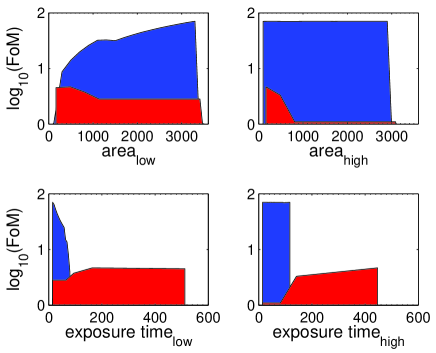
Figure 3: The distribution of survey parameters by FoM for the area (in sq. degrees, top) and exposure time (in minutes, bottom) for surveys observing 800 hours in the low redshift bin in combination with 700 hours in the high redshift bin. The shaded region delimits allowed surveys. The surveys observe either line (blue) or continuum (red) galaxies. The area of the low redshift bin is well determined (3393 sq. degs for line, 371 for continuum), but the area of the high redshift bin is not determined at all because this bin does not add to the FoM.

Table 7 demonstrates that observing either line or continuum galaxies at high redshift does not improve the FoM, no matter what type of galaxies are observed at low redshift. This manifests itself in the flatness of the FoM plots for the high redshift bin area and exposure time in Figure 3, and the corresponding width of the flexibility bars. The ineffectiveness of the high-redshift bin is due to the small energy density of the dark energy at this redshift for our assumed cosmological constant fiducial model, and may change for more general dark energy models.

5.2 Optimal redshift regime

In the previous subsection, we held fixed the limits of the two redshift regimes and the total time spent in each, whilst varying the area and exposure times of surveys for the four different galaxy samples. Here, we address the issue of the optimal redshift range for constraining dark energy models by allowing the total times ($\tau_{low}$ and $\tau_{high}$), the central redshift ($z_{i}$), and width ($dz_{i}$), of the two redshift regimes to vary as free parameters in our MCMC search. We still however impose the global redshift constraints of $0.5<z<1.5$ and $2.5<z<3.5$ to ensure we obtain realistic survey configurations.

The results of this search are presented in Figures 4 and 5, as well as in Table 8. First, we consider a single “low redshift” bin (surveys A for “blue” galaxies and C for “red” galaxies in Table 8), where the mean redshift and redshift widths are allowed to move. Note that now all the survey time is spent at low redshift ($\tau_{low}=1500$ hrs). As seen in Figure 4, these changes in survey time and redshift limits have a marked effect on the FoM, i.e, 218 compared to 72 for blue galaxies and 42 compared to 1.8 for red galaxies. The area of the survey increases in both cases, whilst the optimal redshift increases for the blue galaxies ($z_{low}=0.9\rightarrow 1.1$), and decreases for the red galaxies ($z_{low}=0.9\rightarrow 0.8$).

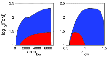
Figure 4: The distribution of survey parameters by FoM for the area and midpoint redshift for a single bin at low redshift for line-emission (blue) and continuum (red) strategies . The shaded region delimits allowed surveys. Note that since there is only one bin, all time is spent observing at this redshift (1500 hours).

We next consider the question of whether a high redshift bin adds to the Figure-of-Merit, and what the optimal splitting of total survey time between the two bins is. We consider the case of two redshift bins (“high” and “low”), where the high redshift galaxies are observed by line emission, and the total survey time is a constraint (i.e. $\tau_{low}+\tau_{high}=\tau_{total}=1500$ hrs). The results are presented in Table 8 and Figure 5.

The addition of a “high redshift” bin for line-emission galaxies (surveys B and D in the table) does not improve the FoM, it in fact gets slightly worse, 176 compared to 207 for a single low-redshift bin of line emission, or doesn’t change, 29 compared to 29 for a single low-redshift bin of continuum emission.

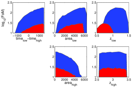
Figure 5: The distribution of survey parameters by FoM as for Fig. 3, with the position and widths of the two redshift bins being allowed to vary. Note that the red colour indicates the galaxy type at low redshift only (continuum), whereas the high redshift bin targets line-emission galaxies in both cases.

Table 8: Best fit survey parameters allowing the redshift bins to move (without and with a line-emission redshift bin at high redshift), with the flexibility bounds in brackets

	Survey
Survey Parameters	A	B	C	D
Low-z bin	Line	Line	Cont	Cont
- $A_{\rm low}$ (sq. degs)	6300 (4500-6300)	5600 (4500-6150)	6300 (3700-6300)	5448 (3100-6000)
- $\tau_{\rm low}$ (hrs)	1500 (-)	1400 (1100-1500)	1500 (-)	1400 (1100-1500)
- $z_{\rm low}$	1.1 (0.95-1.35)	1.08 (0.95-1.35)	0.74 (0.65-0.9)	0.72 (0.65-0.9)
- $dz_{\rm low}$	0.3 (0.12-0.5)	0.35 (0.14-0.48)	0.18 (0.11-0.26)	0.19 (0.11-0.26)
- exp. time (mins)	15	19	15	17
- num. dens $\times 10^{4}$ ($h^{3}$ Mpc-3)	6.5	7.1	3.7	4.5
High-z bin	-	Line	-	Line
- $A_{\rm high}$ (sq. degs)	-	150 (0-1200)	-	43 (0-1200)
- $\tau_{\rm high}$ (hrs)	-	100 (0-400)	-	100 (0-400)
- $z_{\rm high}$	-	3.15 (2.6-3.4)	-	2.9 (2.65-3.35)
- $dz_{\rm high}$	-	0.13 (0.1-0.5)	-	0.27 (0.1-0.5)
- exp time (mins)	-	60	-	240
- num. dens $\times 10^{4}$ ($h^{3}$ Mpc-3)	-	0.13	-	0.35
FoM	207	176	29	29

5.3 Optimal number of redshift bins

The analysis presented in Section 5.2 demonstrated the sensitivity of the FoM to both the location, and number, of redshift regimes, i.e., our optimization clearly preferred a single “low redshift” bin. Therefore, we study here the benefits of splitting this single “low redshift” bin into multiple thinner redshift bins, assuming these thinner bins are contiguous over the full redshift range of the single wider bin. We expect these thinner redshift bins to have worse measurements of $d_{A}(z)$ and $H(z)$, compared to the single wider bin (because their volumes will be smaller), but this disadvantage could be overcome by the increased number of distance measurements available for fitting the cosmological models (we do not consider correlations between the errors of different redshift bins). Therefore, we performed a MCMC search as a function of the number of “low redshift” bins and discovered that the FoM quickly saturated at $\simeq 260$ for all configurations with more than one “low redshift” bins, i.e., the optimal survey would split the single low-redshift regime into two equally–sized bins. These results should be revisited for different dark energy models.

5.4 Global Optimum

We find that the best Figure-of-Merit searching through all possible survey configurations is one which spends all its time at low redshift surveying an area of around 6000 sq. degs, targetting line-emission galaxies (survey A in Table 8). The medium redshift of the bin is about 1.1 and it will stretch from $z\sim 0.8-1.4$. The exposure time is 15 minutes per field-of-view. A additional high redshift bin is disfavoured.

This optimum is not highly peaked, as we can see by looking at Figure 4. The flattening of the FoM curve for area at about 6000 sq. degs and the flat plateau at the top of the $z_{low}$ curve indicates that deviations from these optimal values will result in only small changes in the Figure-of-Merit, also shown by the large width of the flexibility bars in Table 8. This shows that these results are robust against moderate changes in the survey design.

6 External Constraints

In the previous Section we focussed on optimizing the survey parameters to obtain the best constraints on the properties of dark energy, whilst keeping the constraint parameters fixed. We now consider the case where the current constraint parameters are changed or new constraints are added, and the resulting effects on the optimal survey FoM and configuration.

The constraint parameters cannot be considered as simple survey design parameters, as they are built in at an instrument level. Furthermore, the constraint parameters will be unbounded by FoM in one direction. For example a survey that runs for 5 years will always do better than a survey that lasts for only 3 years. However, the behaviour of the FoM will be different for different constraint parameters. The Figure-of-Merit of the best survey will continue to scale as the total survey time is increased, but may quickly asymptote to some maximal value in the case of the number of spectrograph fibres.

We consider three cases: (1) a extra constraint is imposed on the maximum area to be surveyed, motivated by the size of the input photometric catalogue; (2) the number of spectroscopic fibres is changed; and (3) the telescope aperture and field-of-view are changed. Finally, we consider how the optimal design changes if constraints from other dark energy surveys (of both supernovae and baryon acoustic oscillations), which will have been completed by the time that a WFMOS-like instrument is constructed, are included in the analysis.

6.1 Input Photometric Catalogue

The optimal surveys are those with the maximum possible area, surveying thousands of square degrees. However, a spectroscopic survey requires an input catalogue of photometrically pre-selected galaxies. How would the dark energy constraints be affected if the available area of the input catalogue is less than the optimal value?

Looking at Table 8 for a single redshift bin, we see that the flexibility bounds place a lower limit on the total survey area of 3000 sq. degs., compared to the optimal area of 6000 sq. degs. Such imaging surveys, whilst not yet in existence, are in the planning stages (for example the Dark Energy Survey (DES), see Abbott et al. 2005).

6.2 Number of fibres

In this Section we investigate the variation of the optimal Figure-of-Merit with the available number of spectrograph fibres, assuming a single survey bin at low redshift. We consider both line and continuum-emission survey strategies, including both “pessimistic” and “optimistic” versions of the number counts calculation, which correspond simply to decreasing and increasing the predicted number of $z\sim 1$ galaxies by 50%. We assume that the fibres are able to access any part of the field-of-view. We note that this is more challenging for Echidna systems (Kimura et al. 2003), which have a fairly restricted “patrol radius” for each fibre. The results can be seen in Figure 6.

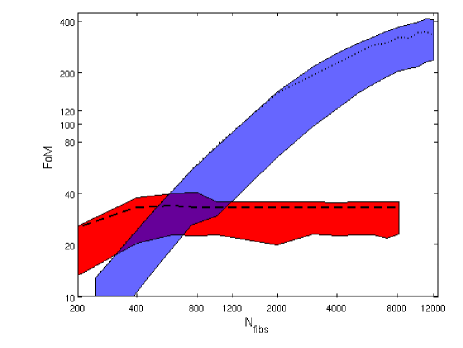
Figure 6: The variation of the FoM of the optimal survey with the total number of spectroscopic fibres, for both line-emission galaxies (dotted curve) and continuum galaxies (dashed curve), for a single bin at low redshift. The line-emission curve does not reach an asymptopic limit before 10,000 fibres, whereas the continuum curve reaches its asymptotic value at around 750 fibres. We also include the effect of varying the number counts models of the galaxies in a band between “pessimistic” and “optimistic” limits (line-emission in blue and continuum-emission in red). This extra freedom does not change the results concerning number of fibres. For a small number of fibres, the optimistic and default models give the same FoM, as the optimal surveys have reached the maximum number of pointings and smallest exposure time, and no more galaxies can be observed. We assume that fibres can access any part of the field-of-view.

The optimal value of the number of fibres for line-emission strategies is around 10,000 for a single low redshift bin. At this point the number density of galaxies sampled is more than sufficient that shot noise is negligible. The optimal value for the continuum case is about 750. We note that the large difference in fibre numbers between the two cases is due to the ability of the line-emission survey to access higher redshifts. These optimal numbers of fibres are not affected by shifting to a “pessimistic” or “optimistic” number counts model.

We note that the optimal survey configuration for 10,000 fibres only obtains successful redshifts for about 6000 galaxies, with the remaining targets possessing emission-line fluxes that fall below the minimum $S/N$ level and produce failed redshifts. Therefore, it is also interesting to consider the most efficient use of fibres. One method of quantifying this “fibre efficiency” is to plot the FoM per fibre as a function of fibre number, as shown in Figure 7. For line-emission galaxies, the most efficient number of fibres judged by this statistic is 2000, but this survey configuration has a significantly lower FoM compared to the optimal survey (151, compared to 328 for 10,000 fibres). A happy medium would be a total of 3000-4000 fibres.

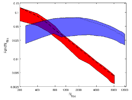
Figure 7: Constructed from the same data as Figure 6, but we now plot FoM/$n_{fibres}$ against the number of fibres, to find the most efficient use of the instrument.

6.3 Telescope Aperture and Field of View

In this Section we consider executing the galaxy surveys using a spectrograph differing from the WFMOS specifications presented in Table 2. We consider three alternate possibilities: reducing the WFMOS field-of-view from $1.5$ deg to $1.0$ deg diameter, using the AAOmega spectrograph on the Anglo-Australian Telescope (AAT), and using the Sloan Digital Sky Survey (SDSS) hardware.

The reduction of the field-of-view is a simple alteration, as it does not affect the exposure time required to obtain the redshift of a galaxy (and thus the number density for a given exposure), but only changes the total number of redshifts taken in a single pointing. Altering the telescope aperture and fibre aperture is a more complex change as it will affect the exposure times. This can be accommodated by changes in the parameters of the number counts calculator. The parameters for the different instruments considered are given in Table LABEL:instruments.

Table 9: Spectrograph parameters for different instruments. These are considered as alternate constraint parameters to those found in Table 2. The de-scope option for the WFMOS FoV is included in brackets.

Instrument	WFMOS	AAOmega	SDSS
Overhead time (mins)	10	5	30
Min time (mins)	15	60	30
$n_{fibres}$	3000	392	640
FoV (diameter in deg)	1.5 (1)	2	3
fibre aperture (arcsec)	1	2	3
effective mirror diameter (m)	8.0	3.5	2.5
Nod and shuffle	Yes	No	No

The smaller apertures and larger fibre diameters of the SDSS and AAOmega systems mean that their exposure times to obtain the same angular source density as a WFMOS survey are longer, but this is partially countered by a larger field-of-view which allows them to survey more of the sky per pointing. We compared the different hardware possibilities by finding the best Figure-of-Merit for a survey with a single bin at low redshift (where all other survey parameters are allowed to vary). The result of the previous section showed that the optimal targetted galaxy population changes with the number of fibres of the instrument, so we also compared targetting red (continuum) and blue (line emission) galaxies at low redshifts. The results are shown in Table 10.

Table 10: Best FoM for surveys conducted on telescopes with the given FoV and Aperture for different galaxy types

Telescope	Aperture	FoV	FoM
/Instrument		diameter	blue	red
Subaru/WFMOS	8m	1.5	207	29
Subaru/WFMOS	8m	1.0	141	16
AAT/AAOMega	3.5m	2	13	21
SDSS	2.5m	3	18	21

We find that line-emitting galaxies are strongly preferred as targets for WFMOS (regardless of field-of-view), whereas red galaxies are marginally preferred for SDSS and AAOmega, which only have a few hundred fibres. This is consistent with the result for WFMOS for a small number of fibres (see Fig. 6), where red galaxies are preferred. We find that the SDSS and AAT are almost equivalent in terms of Figure-of-Merit, as the smaller aperture of the SDSS system (and so longer exposure times) is balanced by the larger field-of-view and number of fibres. Considering the de-scope option of reducing the WFMOS field-of-view to 1 degree diameter, this reduces the survey area by a factor of 2, and thus the FoM drops by almost the same factor (in detail, since the number of fibres is held constant, the fibre density increases, which offsets the loss of area to some extent). In other words, equivalent results will be obtained by a 3-year survey with a 1.5-deg-diameter system and a 4.5-year survey with a 1-deg-diameter system.

6.4 Other Surveys

During the construction period of a WFMOS-like instrument, a number of other dark energy surveys will be performed. These measurements of the angular diameter distance and Hubble parameter in the case of BAO surveys, or luminosity distance in the case of Type Ia Supernovae (SN-Ia) surveys, will have already constrained some of the dark energy parameter space. By including the predictions for these surveys in our analysis, we can determine whether our optimal survey design changes. We consider two surveys that are currently underway: (1) WiggleZ, a baryon acoustic oscillation survey being carried out with the AAOmega spectrograph; and (2) the full five-year SuperNovae Legacy Survey and the Sloan Digitized Sky Survey II Supernova Survey (SNLS-SDSS).

The WiggleZ survey has the following parameters: Area = 1000 sq deg, $z=0.75$, $dz=0.25$, number density $=8.5\times 10^{-4}$ $h^{3}$ Mpc^-3, observing line-emission galaxies (Glazebrook et al. 2007). Using our fitting formula code (Blake et al. 2006) we find that this corresponds to measurement accuracies of 3.1% in $d_{A}$ and 5.2% in $H(z)$. This is easy to include in our optimization, as it counts as an extra measurement at a redshift of 0.75, without any time cost.

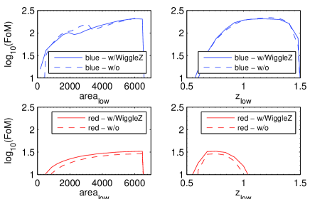
Figure 8: The Figure-of-Merit as a function of area (left) and redshift (right) for a single-bin survey at low redshift using either line emission (top) or continuum emission (bottom) galaxies, with (solid) and without (dashed) the WiggleZ measurement at $z=0.75$.

We find that the inclusion of the WiggleZ measurement has no effect on any of the survey parameters, as shown in Figure 8, as the curves with and without the WiggleZ survey are virtually identical. This is because the WFMOS measurement would produce a much more accurate measurement of dark energy properties.

The SNLS-SDSS SN-Ia survey will find around 1000 Supernovae distributed approximately evenly in the range $0.1<z<1$ (D. Andrew Howell and the SNLS collaboration 2004; SDSS-II Supernovae Survey Fall 2005). The measurement is the apparent magnitude ($m$) of the supernovae, defined as

$$m(z)=5\log_{10}d_{L}(z)+[M+25]\,.$$ (9)

The luminosity distance will give us information about the expansion, but we have the added complication of marginalizing over the absolute magnitude $M$. The supernova surveys therefore do not constrain the Hubble parameter $h$. The Fisher matrix for supernova surveys is (Tegmark et al, 1998; Kim et al, 2004)

$$F_{ij}=\frac{1}{\sigma_{m}^{2}}\int dz\,N(z)\frac{\partial m}{\partial p_{i}}\frac{\partial m}{\partial p_{j}}\,,$$ (10)

where $\sigma_{m}$ is the error in the magnitude and $N(z)$ is the number of SN-Ia in a redshift bin around $z$. We assume 100 SN-Ia in each of ten equally-spaced redshift bins from 0.1 to 1, setting $\sigma_{m}=0.12$. Appendix A details the evaluation of the Fisher matrix elements.

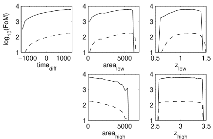
Figure 9: The Figure-of-Merit as a function of the survey parameters for a two-bin survey using line emission galaxies, with (solid) and without (dashed) the SNLS-SDSS SN-Ia measurement over the range $z=0.1-1$. Although the inclusion of the SN-Ia measurement greatly improves the FoM, it has no effect on the distribution of survey parameters with Figure-of-Merit, and does not change the parameters of the optimal survey.

The SN-Ia surveys and the WFMOS BAO survey are approximately equivalent in their effectiveness at investigating the dark energy, with the SN-Ia FoM being 158, compared to the WFMOS FoM of 207. When the two surveys are combined, we find once again that the inclusion of the SN-Ia measurement has no effect on the distribution of survey parameters with Figure-of-Merit, as show in Figure 9. However, the increase in the Figure-of-Merit is marked, improving from $\sim 207$ to $\sim 6250$, equivalent to a shrinkage of error ellipse area of about $\sqrt{6250/207}\simeq 5.5$ times. This is due to the complimentary nature of the two types of measurement.

7 Conclusions

In this paper we have conducted an optimization of the survey parameters of a WFMOS-like survey of the baryon acoustic oscillations in order to best constrain the concordance $\Lambda$CDM model. We use the determinant of the $w_{0},w_{a}$ Fisher matrix of the predicted errors on the dark energy as our Figure-of-Merit to choose between different surveys. We find that when optimizing for a cosmological constant ($\Lambda$) model of the dark energy ($w_{0}=-1$, $w_{a}=0$), a line-emission galaxy selection strategy is preferred over continuum emission. The optimal survey spends all the available survey time (1500 hours in this analysis) observing at low redshift, surveying an area of around 6000 sq. degs. The medium redshift of the bin is about 1.1 and it will stretch from $z\sim 0.8-1.4$. The optimal solutions are not highly peaked, and the flexibility bars are often considerable. Reducing the area by several hundred sq. degs and increasing the target density (for a fixed observing time) does not change the dark energy measurements by a significant amount.

We find that the measurement of the baryon acoustic oscillations in a high redshift ($z=3$) bin is not optimal for testing a $\Lambda$CDM model. This is due to the long exposure times for obtaining redshifts of LBGs compared to $z=1$ galaxies. In addition, the effect of the dark energy on the expansion of the universe is negligible at high redshift (assuming a cosmological constant) and so measuring the BAOs at this redshift (in addition to low redshift) makes only (at best) a small extra contribution to the Figure-of-Merit. If we consider other more exotic dark energy models with non-negligible energy density at high redshift, it may become more important and favoured by the IPSO method. Alternatively, the high-redshift BAOs could be measured with a Lyman-$\alpha$ survey “piggy-backed” on the low-redshift galaxy survey (McDonald & Eisenstein, 2006). However the high redshift part of the survey only serves to cross-check the paradigm and will not improve statistical error bars on the cosmological parameters. Even so, the high redshift bin shouldn’t be ruled out purely on this basis, as it may be responsible for completely new discoveries.

We also examine the optimal instrument design, analyzing the scientific benefit/penalties of different choices. In particular, increasing the number of fibres has a positive effect on the FoM, as more objects can be observed simultaneously, and a higher number density can be achieved for a given exposure time. This FoM increase continues until the number of fibres reaches some optimal value, at which point enough galaxies have been observed to easily beat shot noise effects, and the FoM stops increasing. This optimal value is around 10,000 fibres for line-emission strategies, and 750 for continuum emission. The large difference between the two strategies is due to the ability of the line-emission surveys to reach higher redshifts. We note that since 10,000 fibres only obtains successful redshifts for about 6000 galaxies, compared to most efficient number of fibres by this criterion is 2000. This survey configuration has a significantly lower FoM compared to the optimal survey (151, compared to 328 for 10,000 fibres), and so the optimum would be a value around 3000-4000 fibres. Note that if we were to include the effect of reconstructing the power spectra on small scales (Eisenstein et al. 2006b), this may increase the required number of fibres. Reconstruction increases the performance in measuring the BAOs for any number density, but works especially well at high number densities, and may therefore increase the optimal number density.

We find that including measurements made by other baryon oscillation and supernovae surveys in the total error analysis does not change the optimal survey, indicating that the analysis we do now should remain valid into the medium future.

Finally, we have demonstrated how the IPSO technique can be applied to “realistic” simulations of redshift surveys, including instrumental limitations such as fibre number, repositioning overheads and galaxy number counts models. Since the measurement of baryon acoustic oscillations is one method to measure the dark energy, IPSO could also be applied to the survey & instrumental design that use other methods such as weak lensing, integrated Sachs-Wolfe or cluster number counts, or even those with other science goals.

Appendix A Fisher matrix formalism and model definitions

We use the Fisher matrix formalism to compute the errors on the model parameters $p_{A}$, given the observational errors on the measured quantities $X_{i}$. Here $p_{A}$ includes the optimisation target parameters $\theta$ as well as other nuisance parameters. The Fisher matrix is the curvature at the peak of the likelihood,

$$F_{AB}=\frac{\partial^{2}(-\log{\cal L})}{\partial p_{A}\partial p_{B}}.$$ (11)

Its inverse is a local approximation to the covariance matrix and provides a lower limit for the errors on the model parameters via the Kramer-Rao bound.

We can rewrite the Fisher matrix via the chain rule to depend only on observational quantities,

$$F_{AB}=\sum_{ij}\frac{\partial X_{i}}{\partial p_{A}}F_{ij}\frac{\partial X_{j}}{\partial p_{B}}.$$ (12)

The observational Fisher matrix is taken to be the inverse of the data covariance matrix, $F_{ij}=C_{ij}^{-1}$.

In our case the model parameter vector is $\hat{p}=\{\Omega_{m},\omega_{m}\equiv\Omega_{m}h^{2},w_{0},w_{a}\}$ where the two $w_{i}$ parameters describe the dark energy equation of state $w$, the ratio of the pressure to density. We use the parametrisation

$$w(z)=w_{0}+w_{a}\frac{z}{1+z}.$$ (13)

We also assume that the universe is flat and that the influence of radiation is negligible so that $\Omega_{DE}=1-\Omega_{m}$.

From the observations we recover the comoving distance to redshift $z$, $r(z)$ (from the transverse modes) and its derivative $r^{\prime}(z)$ (from the radial modes). More precisely, we recover $y(z)\equiv r(z)/s$ and $y^{\prime}(z)\equiv r^{\prime}(z)/s$. The quantity $s$ is the comoving sound horizon at last scattering. By using the fitting formula described in a previous paper (Blake et. al, 2006) we also recover the fractional errors $x=\Delta y/y$ and $x^{\prime}=\Delta y^{\prime}/y^{\prime}$ for a given observational setup. We assume that the errors $x$ and $x^{\prime}$ are uncorrelated between each other and between redshift bins. In this case the covariance matrix is diagonal. Expressed in terms of these quantities the Fisher matrix becomes

$$F_{AB} = \sum_{i}\frac{1}{y(z_{i})^{2}}\frac{\partial y(z_{i})}{\partial p_{A}}\frac{\partial y(z_{i})}{\partial p_{B}}\frac{1}{x_{i}^{2}}$$ (15)

$$+\sum_{i}\frac{1}{y^{\prime}(z_{i})^{2}}\frac{\partial y^{\prime}(z_{i})}{\partial p_{A}}\frac{\partial y^{\prime}(z_{i})}{\partial p_{B}}\frac{1}{x_{i}^{{}^{\prime}2}}$$

Here the sums run over the observational bins. Separating $y$ into the contributions due to $r$ and $s$, and writing $D_{A}f\equiv\partial\log(f)/\partial p_{A}$ for the logarithmic derivative of a function $f$ we can write the above formula as

$$F_{AB} = \sum_{i}\frac{\left(D_{A}r(z_{i})-D_{A}s\right)\left(D_{B}r(z_{i})-D_{B}s\right)}{x_{i}^{2}}$$ (17)

$$+\sum_{i}\frac{\left(D_{A}r^{\prime}(z_{i})-D_{A}s\right)\left(D_{B}r^{\prime}(z_{i})-D_{B}s\right)}{x_{i}^{{}^{\prime}2}}$$

It remains to compute $D_{A}r$, $D_{A}r^{\prime}$ and $D_{A}s$.

The comoving distance is given by

$$r^{\prime}(z)=\frac{c}{H(z)}\;,\qquad r(z)=\int_{0}^{z}r^{\prime}(x)dx.$$ (18)

Since we are dealing only with logarithmic derivatives we find that all constants drop out, and we set $c=1$ from now on. For our simplified cosmological model the Hubble parameter is

$$H^{2}(z)=H_{0}^{2}\left({\Omega_{m}}(1+z)^{3}+(1-{\Omega_{m}})f(z;w_{0},w_{a})\right)$$ (19)

The function $f(z;w_{0},w_{a})$ describes the evolution of the energy density of the dark energy and can be integrated directly for our parametrisation of $w(z)$,

$$f(z;w_{0},w_{a}) = \exp\left\{3\int_{0}^{z}\frac{1+w(x)}{1+x}dx\right\}$$ (20)

$$= (1+z)^{3(1+w_{0}+w_{a})}\times$$

$$\exp\left\{-3w_{a}\frac{z}{1+z}\right\}$$

At this point we should rewrite the Hubble parameter in terms of our base parameter set. Specifically we have to replace $H_{0}^{2}=10^{4}{\omega_{m}}/{\Omega_{m}}$. Here we can again neglect the factor $10^{4}$ as it will drop out of the Fisher matrix computation. Eq. (19) is now

$$h(z)^{2}={\omega_{m}}\left((1+z)^{3}+(1/{\Omega_{m}}-1)f(z;w_{0},w_{a})\right).$$ (22)

As the redshift integration for $r(z)$ converges, we know that differentiation with respect to $p_{A}$ and integration over $z$ commute. It is therefore sufficient to calculate $\partial r^{\prime}(z)/\partial p_{A}$. For $r^{\prime}$ we have that $\partial_{A}r^{\prime}(z)=-\partial_{A}h(z)/h^{2}(z)$. Clearly then $D_{A}r^{\prime}(z)=-D_{A}h(z)$. Of course for $D_{A}r(z)$ we need to compute

$$D_{A}r(z)=\frac{\int_{0}^{z}\partial_{A}r^{\prime}(x)dx}{\int_{0}^{z}r^{\prime}(x)dx}.$$ (23)

We will now derive explicitely expressions for all $\partial_{A}r^{\prime}$.

$$\partial_{\omega_{m}}r^{\prime}(z) = -\frac{1}{2{\omega_{m}}h(z)}=-\frac{1}{2{\omega_{m}}}r^{\prime}(z)$$ (24)

$$D_{\omega_{m}}r^{\prime}(z) = -\frac{1}{2{\omega_{m}}}$$ (25)

(up to an irrelevant constant pre-factor). In this case we can perform formally the $z$ integration and find

$$D_{\omega_{m}}r(z)=-\frac{1}{2{\omega_{m}}}=D_{\omega_{m}}r^{\prime}(z).$$ (26)

For the next term we get

$$\partial_{\Omega_{m}}r^{\prime}(z)=-\frac{1}{2}\frac{\partial_{\Omega_{m}}h(z)^{2}}{h(z)^{3}}=\frac{1}{2}\frac{{\omega_{m}}f(z;w_{0},w_{a})}{{\Omega_{m}}^{2}h(z)^{3}}.$$ (27)

There do not seem to be any straightforward simplifications. As always, $D_{\Omega_{m}}r^{\prime}(z)=h(z)\partial_{\Omega_{m}}r^{\prime}(z)$. The derivative with respect to the dark energy parameters $w_{i}$ is just the same as before, except that we differentiate the $f$ instead,

$$\partial_{w_{i}}r^{\prime}(z) = -\frac{1}{2}\frac{\partial_{w_{i}}h(z)^{2}}{h(z)^{3}}$$ (28)

$$= -\frac{1}{2}\frac{{\omega_{m}}(1/{\Omega_{m}}-1)\partial_{w_{i}}f(z;w_{0},w_{a})}{h(z)^{3}}$$

where

$$\partial_{w_{0}}f(z;w_{0},w_{a}) = 3\log(1+z)f(z;w_{0},w_{a})$$ (29)

$$\partial_{w_{a}}f(z;w_{0},w_{a}) = 3\left(\log(1+z)-\frac{z}{1+z}\right)f(z;w_{0},w_{a})$$ (30)

For the logarithmic derivative of $s$ we use a numerical differentiation of the following formulae: the sound horizon at recombination is given by

$$s=\frac{c}{\sqrt{3}}\frac{1}{H_{0}\Omega_{m}^{1/2}}\int_{0}^{a_{r}}\frac{da}{(a+a_{\mathrm{e}qu})^{1/2}}\frac{1}{(1+R)^{1/2}}\,,$$ (31)

which can be evaluated (Efstathiou and Bond 1999) and gives

$$s = \frac{4000}{\sqrt{\omega_{b}}}\frac{\sqrt{a_{\mathrm{e}qu}}}{\sqrt{1+\eta_{\nu}}}$$ (32)

$$\ln\left\{\frac{[1+R(z_{r})]^{1/2}+[R(z_{r})+R_{\mathrm{e}qu}]^{1/2}}{1+\sqrt{R_{\mathrm{e}qu}}}\right\}{\mathrm{M}pc}\,,$$

where $\eta_{\nu}=0.6813$ is the ratio of the energy density in neutrinos to the energy in photons. The parameter $R=3\rho_{b}/4\rho_{\gamma}$ is numerically

$$R(a)=30496\omega_{b}a\,.$$ (33)

The scale factor at which radiation and matter have equal density is

$$a_{\mathrm{e}qu}^{-1}=24185\left(\frac{1.6813}{1+\eta_{\nu}}\right)\omega_{m}$$ (34)

and the redshift of recombination, $z_{r}$, is given by the following fitting-formula (Hu & Sugyiama 1996)

$$z_{r} = 1048\left(1+0.00124\omega_{b}^{-0.738}\right)\left(1+g_{1}\omega_{m}^{g_{2}}\right)\,,$$ (35)

$$g_{1} = 0.0783\omega_{b}^{-0.238}\left(1+39.5\omega_{b}^{0.763}\right)^{-1}\,,$$ (36)

$$g_{2} = 0.560\left(1+21.1\omega_{b}^{1.81}\right)^{-1}\,.$$ (37)

References

- [] Abbott, T., et al. [Dark Energy Survey Collaboration], 2005 (astro-ph/0510346.)
- [] Albrecht, A. and Bernstein, G., 2006a, preprint(astro-ph/0608269).
- [1] Albrecht, A., et al., 2006b, “Report of the Dark Energy Task Force,” preprint(astro-ph/0609591).
- [] Arnouts, S., 2005, ApJ. 619 L43-L46
- [] Barden, S., et al (The WFMOS feasibility study team), 2005, private communication
- [] Bassett, B.A., Corasaniti, P.S., Kunz, M., 2004, ApJ. 617 L1-L4
- [] Bassett B. A., 2005, Phys. Rev. D 71 083517.
- [] Bassett, B. A., Parkinson, D. and Nichol, R. C., 2005, ApJ. 626 L1
- [] Bassett, B. A., Nichol, R. C. and Eisenstein, D. J. 2005, astro-ph/0510272,
- [] Blake, C. and Glazebrook, K., 2003, ApJ. 594 665.
- [] Blake, C., Abdalla, F. B., Bridle, S. L., and Rawlings, S., 2004 New Astron. Rev. 48 1063
- [] Blake, C., Parkinson, D., Bassett, B. A., Glazebrook, K., Kunz, K. and Nichol, R. C., 2006, MNRAS, 365, 255
- [] Cannon, R., et al., 2006, MNRAS, 372, 425
- [] Carroll, S. M., 2001, Living Rev. Rel. 4, 1, astro-ph/0004075.
- [] Cole S. et al., 2005, MNRAS, 362, 505
- [] Carloni, S., Dunsby, P.K., Capozziello, S., Troisi, A., 2005, Class. Quant. Grav. 22, 4839.
- [] Cerny, V., 1985, J. Opt. Theory Appl., 45, 1, 41-51
- [] Chevallier, M., Polarski D., 2001, Int. J. Mod. Phys. D10, 213
- [] Cooper M. C.,S et al 2006 Mon.Not.Roy.Astron.Soc. 370, 198
- [] Corasaniti, P.S., Kunz, M., Parkinson, D., Copeland, E.J., Bassett, B.A., 2004, Phys.Rev. D 70 083006
- [] Damour, T., Kogan, I. I. & Papazoglou, A., 2002, Phys. Rev. D66, 104025.
- [] Deffayet, C., Dvali, G. & Gabadadze, G., 2002 Phys. Rev. D65, 04402.
- [] Efstathiou G. & Bond J.R., 1999, Mon.Not.Roy.Astron.Soc. 304, 75
- [] Eisenstein, D.J., et al., 2001, Astron. J., 122, 2267
- [] Eisenstein, D. J. , and White, M., 2004, Phys.Rev. D 70 103523
- [] Eisenstein, D. J. , et al., 2005, ApJ 633 560.
- [] Eisenstein, D. J. , Seo, H, and White, M., ApJ, 2006, submitted (astro-ph/0604361)
- [] Eisenstein, D. J. , Seo, H, Sirko, E., and Spergel, D., 2006b,, submitted (astro-ph/0604362)
- [] Glazebrook, K., Baldry, I., Moos, W., Kruk, J., McCandliss, S., 2005a, New Astron. Rev., 49, 374.
- [] Glazebrook, K., Eisenstein, D.J., Dey, A., Nichol, R.C., The WFMOS Feasibility Study Dark Energy Team, 2005b, preprint(astro-ph/0507457)
- [] Glazebrook, K. and Blake, C., 2005, ApJ. 631 1.
- [] Glazebrook, K., et al., 2007, astro-ph/0701876.
- [] Hastings, W. K., 1970, Biometrika, 57 97-109
- [] Hill, G., et al., 2005, New Astron. Rev., submitted
- [] Hopkins, A., 2004, ApJ, 615, 209
- [] Howell, D. A. [The SNLS Collaboration], 2004, astro-ph/0410595.
- [] Hu, W. and Haiman, Z. 2003, Phys.Rev. D 68 063004
- [] Hu, W. and Sugiyama, N., 1996 Ap J, 471, 542.
- [] Kim, A. G., Linder, E. V., Miquel, R. and Mostek, N., 2004 Mon. Not. Roy. Astron. Soc. 347 909.
- [] Kimura, M., et al., 2003, Proceedings of the SPIE, 4841, 974
- [] Kirkpatrick, S., Gelatt Jr., C. D., Vecchi, M. P., 1983, Science, 220, 4598, 671-680.
- [] Krauss, L. M., and Turner, M. S., 1995, Gen. Rel. Grav. 27 1137.
- [] Liddle, A.R., Mukherjee, P., Parkinson D. and Wang, Y., 2006, Phys. Rev. D 74 123506
- [] Linder, E. V., 2003, PRL 90, 091301.
- [] McDonald, P., and Eisenstein, D., 2006 astro-ph/0607122.
- [] Metropolis, N., Rosenbluth, A.W., Rosenbluth, M.N., Teller, A.H., and Teller, E., 1953, J. Chem. Phys. 21, 1087
- [Miller et al.(2001)] Miller, C. J., Nichol, R. C., & Batuski, D. J. 2001, ApJ, 555, 68
- [] Padmanabhan, N., et al., 2006, MNRAS, submitted (astro-ph/0605302)
- [] Perlmutter, S. et al., 1999, ApJ, 517, 565
- [] Peterson, J. B., Bandura, K., and Pen, U. L., 2006, astro-ph/0606104.
- [] Ratra, B., & Peebles, P. J. E., 1988, Phys. Rev. D 37, 3406
- [] Reiss, A. G., et al., 1998, Astron. J., 116, 1009
- [] The Sloan Digital Sky Survey Supernova Survey, 2005, http://sdssdp47.fnal.gov/sdsssn/pages/sdsssn-main.html
- [] Seo, H.J. and Eisenstein, D.J., 2003, ApJ 598 720.
- [] Shapley, A. E., Steidel, C. C., Pettini, M., and Adelberger, K. L., 2003, ApJ 588 65.
- [] Steidel, C. C., Adelberger, K. L., Giavalisco, M., Dickinson, M., and Pettini, M., 1999, ApJ 519 1
- [] Tegmark, M., Eisenstein, D. J. and Hu, W., 1998, astro-ph/9804168
- [] Willmer, C. N. A., et al., 2005, astro-ph/0506041
- [] Wetterich, C., 1988, Nuclear Phys. B 302, 668