A snapshot of the inner dusty regions of a R CrB-type variable

Abstract

Context. R Coronae Borealis (R CrB) variable stars are suspected to sporadically eject optically thick dust clouds causing, when one of them lies on the line-of-sight, a huge brightness decline in visible light. Direct detections with 8-m class adaptive optics of such clouds located at about 0.2-0.3 arcsec from the centre ($\sim$1 000 stellar radii) were recently reported by de Laverny & Mékarnia (2004) for RY Sgr, the brightest R CrB of the southern hemisphere.

Aims. Mid-infrared interferometric observations of RY Sgr allowed us to explore the circumstellar regions much closer to the central star ($\sim$20-40 mas) in order to look for the signature of any heterogeneities and to characterize them.

Methods. Using the VLTI/MIDI instrument, five dispersed visibility curves in the N band were recorded in May and June 2005 with different projected baselines oriented towards two roughly perpendicular directions. The large spatial frequencies visibility curves exhibit a sinusoidal shape whereas, at shorter spatial frequencies visibility curves follow a Gaussian decrease. These observations are well interpreted with a geometrical model consisting in a central star surrounded by an extended circumstellar envelope in which one bright cloud is embedded.

Results. Within this simple geometrical scheme, the inner 110 AU dusty environment of RY Sgr is dominated at the time of observations by a single dusty cloud which, at 10$\mu$m represents $\sim$10% of the total flux of the whole system, slightly less that the star flux. The cloud is located at about 100 stellar radii (or $\sim$30 AU) from the centre toward the East-North-East direction (or the symmetric direction with respect to centre) within a circumstellar envelope which FWHM is about 120 stellar radii. This first detection of a cloud so close to the central star, supports the classical scenario of the R CrB brightness variations in the optical spectral domain and demonstrates the feasibility of a temporal monitoring of the dusty environment of this star at a monthly scale.

1 Introduction

R Coronae Borealis (R CrB) variable stars are Hydrogen-deficient supergiants exhibiting erratic variabilities. Their visual light-curve is indeed characterized by unpredicted declines of up to 8 magnitudes with time-scale of weeks, the return to normal light being much slower (see Clayton, cla96 (1996), for a review). It has been accepted for decades that such fading could be due to obscurations of the stellar surface by newly formed dusty clouds. Over the years, several indices confirming this scenario were reported although no direct detections of such clouds have been performed. Recently, NACO/VLT near-infrared adaptive optics observations by de Laverny & Mékarnia (lav04 (2004), Paper 1 hereafter) detected clear evidences of the presence of such clouds around RY Sgr, the brightest R CrB variable in the southern hemisphere. New informations about the inner circumstellar regions of these stars were derived as, for instance, (i) several bright and large dusty clouds are present around R CrB variables, (ii) they have been detected in any directions at several hundred stellar radii of RY Sgr, (iii) they can be as bright as 2% of the stellar flux in the near-infrared,… This was the first direct confirmation of the standard scenario explaining R CrB variable stars light variations by the presence of heterogeneities in their inner circumstellar envelope.

However, the precise location of the formation of such dust clouds is still unclear. The brightest cloud detected in Paper 1 indeed lies at several hundred stellar radii from the center but it was certainly formed much closer. This cannot help to disentangle between the two commonly proposed scenarios regarding the location of the dust formation in the vicinity of R CrB variable stars in order to explain their fadings: either the dust is formed very close to the stellar surface ($\sim 2\leavevmode\nobreak\$R_∗ or even less) above large convection cells or it is formed in more distant regions at $\sim 20\leavevmode\nobreak\$R_∗ where the temperature is lower to form dust more easily (see Clayton cla96 (1996) and Feast feast (1997)). Nothing is also known about the physical and chemical properties of these clouds, witnesses of nucleation processes in a rather hot environment. Indeed, the temperature of the layers where they are formed is certainly too high for classical dust formation theories and departures from the chemical and thermodynamical equilibria have therefore to be invoked.

In the present Letter, we report on the interferometric detection of a dusty cloud in the very inner environment of RY Sgr, i.e. in regions located about one-tenth of the distance reported in Paper 1. We present in Sect. 2 the observations and their reduction. The interpretation of the collected visibility curves with a geometrical model is described in Sect. 3. We then validate the adopted model with respect to more complex geometries of the circumstellar environment of RY Sgr. In the last section, we finally discuss our results within the framework of our understanding of R CrB variable stars variability.

2 Observations and data reduction

N-band interferometric data of RY~Sgr were collected in 2005 with the VLTI/MID-infrared Interferometric instrument (MIDI; Leinert et al. lei03 (2003)). Seven runs were executed, using two different telescope pairs (UT1-UT4 and UT3-UT4) and five different baselines. Their orientations are shown in Fig. 1 (top panel). All observing runs were collected under rather good atmospheric conditions. The observations were executed in the so-called High-Sens mode, with 4 templates: acquisition, fringe search, fringe tracking, and photometry. These templates provide, in addition to the dispersed (7.5–13.5 $\mu$m) correlated flux visibilities, N-band adaptive-optics corrected acquisition images and spectro-photometric data for each baseline. We used the grism for wavelength dispersion ($\lambda/\Delta\lambda$=230) and HD~177716 as interferometric, spectrophotometric and imaging calibrator. The observing log is summarized in Table 1.

Table 1: MIDI observations log of RY Sgr and its calibrator.

		RY Sgr			HD 177716
Base	Date	UT Time	Proj. baseline		UT Time
			length	PA
			(m)	(deg)
UT3-4	2005 May 26	$e$   06:01-06:11	57	98	04:54-05:04
		$g$   10:11-10:21	57	135	10:36-10:46
UT1-4	2005 June 25	$a$   03:01-03:10	122	34	02:28-02:36
		$b$   03:12-03:20	123	36	03:44-03:52
		$c$   06:18-06:26	128	65	05:52-06:00
	2005 June 26	$d$   06:42-06:50	125	68	06:19-06:28
UT3-4	2005 June 28	$f$   05:28-05:36	62	110	05:05-05:13

Note: For baseline labels a-g, see Fig. 1.

The observations have been reduced using the MIA software. The fringe tracking of baselines $a$ and $c$ was not satisfactory and good scans were carefully selected based on the histogram of Fourier-Amplitude. The error on the visibilities were estimated by examining level and shape fluctuations of several calibrator visibility curves collected $\pm 2$ hours around every RY Sgr observations. We note that the uncertainties on the visibilities are mostly achromatic and are dominated by the fluctuations of the photometry between the fringe and photometric measurements. The error on the spectral shape of the visibility is smaller than 2% of the visibilities and is considered in the following as an important constraint of the model fitting process. The visibility curves are shown in Fig. 1. The MIDI spectrum of RY Sgr was calibrated using a template of HD 177716 (Cohen et al. coh99 (1999)) and a mean flux error of 12% was estimated from the level fluctuations of all collected spectra. The MIDI spectrum of RY Sgr is similar to the ISO one, but about 25% fainter (probably due to photometric variations and the smaller field-of-view of MIDI). Both spectra exhibit a slow decline between 7.5 and 13.5$\mu$m, compatible with a continuum dominated by hot dust emission. Finally, we processed the 8.7 $\mu$m acquisition images of a single 8m telescope (the FWHM of the beam is 225 mas) by using a shift and add procedure, and found that RY Sgr is unresolved. Moreover, no structures were resolved in these N-band images with a field-of-view of $\sim$2” and a rather low dynamics ($\sim$20-40).

3 Interpretation of the visibility curves

Figure 1 shows the visibility curves as a function of spatial frequency and position angle (PA). Let us recall that the shapes of these curves are determined both by an apparently monotonic change of the object geometrical characteristics between 7.5 and 13.5 $\mu$m and the linear decrease of the resolving power of the interferometer with wavelength. Nevertheless, in a first-order analysis, we neglect any variations with wavelength of the source geometry and tried to fit the curves with simple monochromatic geometric models. This approach gives us fundamental constraints to determine the global morphology of this object in the N-band. Morphological variations with wavelength will be discussed hereafter.

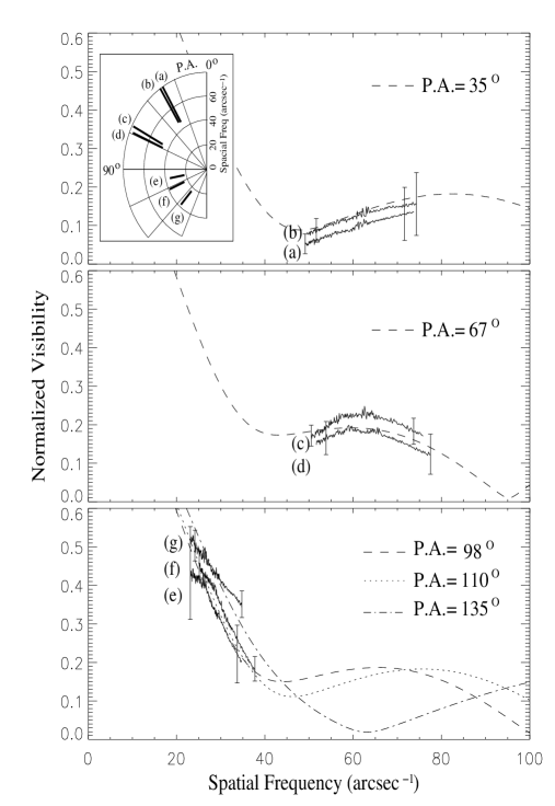
Figure 1: Observed visibilities as a function of spatial frequency and PA. The chart of the observed baselines, representing their projected lengths and PAs, is shown at the top-left corner, with the same labels as in Table 1. The different PAs are also indicated in each panel. The total error bars on the visibilities are shown at each curve extremities in order to illustrate their mean variations as a function of wavelength. The non-solid curves represent PA sections of the theoretical fit with parameters described in Sect. 3 and neglecting any morphological variations with wavelength.

We identify in the observed visibility curves two main signatures. At low spatial frequencies and PA $>$ 90° (baselines labeled $e$ to $g$), the visibility curves have a Gaussian shape while, at higher spatial frequencies and PA $<$ 90° (projected baselines labeled $a$ to $d$), they follow a sinusoidal shape, typical of a two-component signature. These interferometric signatures can be easily interpreted with a geometrical model consisting in a central star and a cloud (the sinusoidal component in the Fourier space), embedded within an extended circumstellar envelope (the Gaussian component).

We calculated theoretical visibility curves for this geometrical model and adjusted its parameters to obtain the most reasonable fit. Let us recall that the errors on the shape of the visibility curves are rather small compared to those on their level. We have therefore given a larger weight for the curve shapes than for their levels to adjust the fit. In this way, we estimated a separation for the cloud of 16$\pm 1$ mas from the central star and a PA of 75°$\pm$10°(modulo 180°, because of the central symmetry of the $u$-$v$ plane). We estimated the FWHM of the Gaussian CSE to be 18$\pm 3$ mas. The central star contributes to 10%$\pm 2\%$ of the total N-band flux of the whole system, close to the cloud contribution (8%$\pm 2\%$). The best fit of the visibility curves (with no morphological variations with wavelength, in particular the relative fluxes between its three components) for these parameter values are shown in Fig. 1.

In a more detailed analysis, we considered possible spectral variations of the model parameters. The modeled visibilities are displayed as a function of wavelength for each observed baseline in Fig. 2. We started by assuming that the estimated distance between the cloud and the centre as its PA have to be constant within the full N-band. The parameters that are allowed to vary in the observed wavelength range were the FWHM of the envelope and the relative fluxes of the star, the cloud, and the envelope, using the first order analysis presented above as a starting point. Very good fits were found with parameter values close to those given in the global analysis, confirming this first solution. In addition, we also found that the CSE FWHM slightly grows from 17 to 19 mas (within uncertainty of $\pm$3 mas) toward larger wavelengths, whereas no significant variation of the stellar and cloud fluxes were observed. Actually, although smaller errors on the visibility curves would help, there is a degeneracy when estimating any spectral variation of the flux of each component with the simple geometrical model considered above. For instance, we see in Fig. 1 that the shapes of the visibility curves $c$ and $d$ are slightly more bent than their theoretical fit. They could be better fitted either by slightly decreasing the stellar flux with increasing wavelength or by slightly increasing the cloud or the CSE contributions with increasing wavelength. A more complete coverage of the observed (u,v) plane is required to disentangle this degeneracy.

Figure 2: Visibility curves as a function of wavelength for the different baselines. Their respective lengths and PAs are indicated in each panel. The total error bars on the visibilities are shown at each curve extremities in order to illustrate their mean variations as a function of wavelength. Best theoretical fits (taking into account any morphological variations with wavelength, see end of Sect. 3) are shown as dashed lines.

4 Validity of the proposed model

Since the five collected baselines cover almost the whole (u,v)-plane, we can safely claim that we have detected the brightest clump in the dusty CSE of RY Sgr. However, the geometry of this CSE could be more complex than described above. We therefore discuss here the effects on the visibility curve of some departures in the proposed model.

First, the smoothness of the visibility curves leads us to discard the hypothesis of a dusty environment filled by several more or less bright clumps. Indeed, any other heterogeneities in the CSE would contribute with rather small perturbations to visibilities, slightly changing the shapes and levels of the curves. In order to test this hypothesis, we thus analysed the effects of the presence of another unresolved clump onto our best model. We then estimated in which conditions it could be confidently detected with the present dataset. Assuming the values estimated in Sect. 3 for the stellar flux and for the CSE flux and size, we found that none of the following heterogeneities would have been distinguishable in addition to the already detected cloud: (i) any cloud closer than typically 3-4 mas from the star because of the limited projected baselines ($\sim$130 m), (ii) any cloud closer than typically 3-4 mas around the main clump at the same PA, or (iii) any clump fainter than $\sim$1-2% of the total flux and located at a typical distance of 5-60 mas from the central star (depending on PA). We also point out that the circumstellar layers located beyond 60 mas are too extended in order to be efficiently explored with the MIDI instrument.

As another verification, we can also see in Fig. 1 that the visibility curves $e$ and $f$ with the lower spatial frequency range are almost straight and smooth and that the sinusoidal contribution is noticeable only at larger frequencies. Thus, any bright cloud located at a larger separation than estimated before would produce, in these two visibility curves, a sinusoidal modulation that is not observed. This would also not reproduce the relatively smoothed shape of the visibility curves $a$ and $b$. Therefore, we are confident in claiming that the contribution of an unique cloud as described in Sect. 3 well fits simultaneously the five visibility curves. Any contribution from any other structure must be much fainter than the main cloud already detected.

The strongest departure of the model with the observed visibilities is seen in curve $g$, the only dataset recorded in May 2005. We investigated whether this departure could be explained by a displacement of the cloud. Considering a typical escape velocity of 275 km s^-1 (Clayton et al. cla03 (2003)) for RY Sgr and a distance of about 1.9 kpc (see Paper 1), we estimate that this cloud could have moved radially by about 2-3 mas in one month but we found that such a displacement does not strongly affect the theoretical visibility curves. Another option is to add to the geometrical model a second cloud with about 5% of the total flux, at a separation of about 30 mas from the central star, and a PA of about 135°. This putative cloud has to be fainter than about 2% one month later in order to be compatible with the other visibility curves. This may indicate a large dilution of the cloud but the lack of data at high spatial frequencies for PA $>$ 90° does not allow us to clearly verify that possibility.

Finally, we point out that the inclusion of any additional features to the geometrical model could certainly help to better adjust the shapes of the theoretical visibility curves but without providing more precise information. Indeed, the more we increase the complexity of a geometrical model the more degenerated its parameters remain. In any case, any other features that could be present in the CSE of RY Sgr would probably be faint or very close to the central star, contributing only by small perturbations to the visibility curves.

5 Discussion

The collected VLTI/MIDI observations are well interpreted with the simple geometrical model of the dusty environment of RY Sgr described in Sect. 3. Owing to this unprecendented study, we can claim that we have explored with a dynamic range better than 20 the inner 60 mas of the RY Sgr environment. That corresponds to about 110 AU (following Paper 1, we assume a distance of about 1.9 kpc and a photospheric angular radius of $\sim$0.15 mas for the central star). We can estimate that the CSE has a FWHM of about 120 R_∗, or $\sim$35 AU and the detected cloud lies at about 100 R_∗ from the central star ($\sim$ 30 AU). This is the closest dusty cloud ever detected around a R CrB-type variable since the first direct detection with the ESO/NACO instrument (see Paper 1). However, such a distance is still too large to disentangle between the two different scenarios proposed for the formation location of dusty clouds around R CrB variables, either at $\sim$2 R_∗ or $\sim$20 R_∗ from the central star. Interferometric observations with larger baselines and at smaller wavelength could help to settle this issue. Using longer baselines in mid-IR is not an easy task: RY Sgr can safely be observed with the VLTI 1.8m Auxiliary Telescopes with baselines up to $\sim$50m, then the correlated flux drops below the MIDI sensitivity limit. Observing at shorter wavelengths with the VLTI/AMBER near-IR recombiner appears to be a better solution. The clouds close to the star should be hotter, improving slightly the contrast, the spatial resolution is strongly increased and the accuracy better than in the N band. Moreover, the closure phase provided by the use of three telescopes simultaneously is a powerful additional constraint, helping for the time monitoring of this kind of objects.

Moreover, assuming an improbable maximum value of about 275 km s^-1 for the velocity projected on the sky of the detected cloud, one can estimate that its ejection occurred more than $\sim$6 months before the epoch of the observations. We found in the AAVSO light-curves of RY Sgr that between early 2002 and the time of our observations two dimming events occurred about 8 and 6 months before the VLTI observations. Their durations were around 40 days and 4 months, and their recovering to maximum light took about 10 days and 2–3 months, respectively. The cloud detected with MIDI was probably not one of those responsible for the dimming reported by AAVSO since this would require too fast a displacement between the line-of-sight (epoch of the minimum of brightness in the optical) and its location at the date of the MIDI observations. The detected cloud could, however, be related to a series of ejections that produced the dimmings seen in the AAVSO light-curves. With such an hypothesis, R CrB-type variables could experience intense periods of material ejection. And, only part of the lost matter was up to now detected during a dimming episode.

Finally, we emphasize that the observations presented here represent a snapshot obtained within one month, June 2005. We still do not know how the detected structures evolve with time, what is their radial velocity compared to the one of the dusty wind and how long are they steady. Since dust clouds are detected rather far from the central star, we suspected in Paper 1 that they are steady over periods of a few years. They probably move away from the central star leading to less obscuration of the stellar surface and the return to normal light would then not be caused by the evaporation of the clouds close to the stellar photosphere as it has been suggested. Time series of visibility curves collected over several months could give crucial informations about any displacement of the heterogeneities found around R CrB variables. This would definitively prove that (i) a dimming event would be related to an ejection of a dusty cloud on the line-of-sight and to a sporadic ejection of stellar material towards any other direction and, (ii) the duration of the return to maximum of brightness would simply result from the displacement of a cloud away from the line-of-sight.

- (1) Clayton, G.C. 1996, PASP, 108, 225
- (2) Clayton, G.C., Geballe, T.R., & Luciana, L. 2003, ApJ, 595, 412
- (3) Cohen, M., Walker R.G., Carter B., et al. 1999, AJ 117, 1864
- (4) de Laverny, P., Mékarnia, D. 2004 A&A, 428, L13, Paper 1
- (5) Feast, M.W., 1997, MNRAS 285, 339
- (6) Leinert Ch., et al., 2003, Msngr, 112, 13