Probing the Coupling between Dark Components of the Universe

Zong-Kuan Guo,^a, Nobuyoshi Ohta^a, and Shinji Tsujikawa^b,
a Department of Physics, Kinki University, Higashi-Osaka, Osaka 577-8502, Japan
^b Department of Physics, Gunma National College of Technology, Gunma 371-8530, Japan

Abstract

We place observational constraints on a coupling between dark energy and dark matter by using 71 Type Ia supernovae (SNe Ia) from the first year of the five-year Supernova Legacy Survey (SNLS), the cosmic microwave background (CMB) shift parameter from the three-year Wilkinson Microwave Anisotropy Probe (WMAP), and the baryon acoustic oscillation (BAO) peak found in the Sloan Digital Sky Survey (SDSS). The interactions we study are (i) constant coupling $\delta$ and (ii) varying coupling $\delta(z)$ that depends on a redshift $z$, both of which have simple parametrizations of the Hubble parameter to confront with observational data. We find that the combination of the three databases marginalized over a present dark energy density gives stringent constraints on the coupling, $-0.08<\delta<0.03$ (95% CL) in the constant coupling model and $-0.4<\delta_{0}<0.1$ (95% CL) in the varying coupling model, where $\delta_{0}$ is a present value. The uncoupled $\Lambda$CDM model ($w_{X}=-1$ and $\delta=0$) still remains a good fit to the data, but the negative coupling ($\delta<0$) with the equation of state of dark energy $w_{X}<-1$ is slightly favoured over the $\Lambda$CDM model.

PACS number(s): 98.80.Es, 98.80.Cq

I Introduction

Recent observations of Supernova Ia (SNIa) suggest that the universe has entered a stage of an accelerated expansion with a redshift $z\lesssim 1$ rie98 ; per99 ; ast05 . This has been confirmed by precise measurements of the spectrum of the Cosmic Microwave Background (CMB) anisotropies spe03 ; spe06 as well as the baryon acoustic oscillations (BAO) in the Sloan Digital Sky Survey (SDSS) luminous galaxy sample eis05 . As is well known, all usual types of matter with positive pressure generate attractive forces, which decelerate the expansion of the universe. Given this, a dark energy component with negative pressure was suggested to account for the invisible fuel that drives the current accelerated expansion (see Refs. review ; CST for reviews).

The simplest candidate for dark energy is a cosmological constant $\Lambda$ (vacuum energy), which corresponds to a constant equation of state $w_{X}=-1$. This model, the so-called $\Lambda$CDM, provides an excellent fit to a wide range of astronomical data so far. However, in such a model there exists a theoretical problem of cosmic coincidence: why is the vacuum density comparable with the critical density at the present epoch in the long history of the universe? One possible approach to alleviating this problem is to assume that the “cosmological constant” is not a constant but is a dynamical component with a slowly evolving and spatially homogeneous scalar field called quintessence quin (see Refs. early for early works and Refs. rec for the reconstruction of quintessence potentials). In such models the resolution of the cosmic coincidence problem typically leads to a fine-tuning of model parameters.

Given the fact that the amount of dark matter is comparable to that of dark energy in the present universe, it is natural to consider an interaction between the two components. Originally cosmological consequences of a scalar field coupled to the matter were studied in Ref. coupleearly . Amendola ame00 considered interaction between a quintessence field $\phi$ and dark matter with a coupling $Q$ that satisfies the relation $T^{\mu}_{\nu(\phi);\mu}=QT_{(m)}\phi_{;\mu}$ between energy momentum tensors. In fact this type of interaction appears in the context of scalar-tensor theories stensor , $f(R)$ gravity models fR , varying mass dark matter/neutrino models Come ; Huey ; das05 ; neutrino and phantom dark energy models guo04 . Interestingly the equation of state of dark energy can extend to the region $w_{X}<-1$ if the mass of dark matter depends on a quintessence field Huey ; das05 . The presence of the coupling can also provide an accelerated scaling attractor along which the ratio of the energy densities of dark energy and dark matter is a constant. Then this may be useful to solve the coincident problem because the present universe can be a global attractor with a dark energy fraction $\Omega_{X}\simeq 0.7$.

However, the coupling $Q$ to realize the accelerated scaling attractor is too large to ensure the presence of a standard matter dominated epoch ame00 . In fact there exists the so-called “$\phi$ matter-dominated epoch” ($\phi$MDE) during which an effective equation of state is given by $w_{\rm eff}=2Q^{2}/3$ ame00 ; CST ; GNST . Amendola ame00 showed that the coupled quintessence model with an exponential potential is not consistent with observational data of CMB unless the coupling $Q$ is smaller than the order of 0.1, but in this case there is no scaling accelerated attractor. Instead the system finally approaches a scalar-field dominated attractor with $w_{\rm eff}=-1$ and $\Omega_{X}=1$, in which case the coincident problem is not solved.

There are many other scalar-field dark energy models such as K-essence, tachyon, phantom and dilatonic ghost condensates. For a general Lagrangian density $p(\phi,X)$ with a kinetic term $X=-(1/2)(\nabla\phi)^{2}$ and a constant coupling $Q$, the existence of scaling solutions required to solve the coincident problem restricts the Lagrangian density to the form $p=X\,g(Xe^{\lambda\phi})$, where $g$ is an arbitrary function and $\lambda$ is a constant Piazza . Recently it has been shown that for the vast class of this generalized Lagrangian that include most of scalar-field dark energy models, the matter era is not followed by the accelerated scaling attractor AQTW . Thus it is still a challenging task to construct coupled scalar-field models which can solve the coincidence problem without using fine-tuned varying couplings stationary .

Since the origin of dark energy is not yet known, there are several different approaches dal01 ; zim01 ; maj04 ; Wei ; ame06 to implementing couplings without restricting to scalar-field models (see also Refs. Pavo -man05 for a number of interesting aspects of interacting dark energy). The approach we adopt in this paper is to introduce an interaction of the form $\Gamma\rho_{m}$ on the rhs of conservation equations, see (2) and (3). While this is basically a fluid description of dark energy, Eqs. (2) and (3) include the aforementioned scalar-field coupling by setting $\Gamma=Q\dot{\phi}$. Since the interaction rate $\Gamma$ measured by the Hubble rate $H$ is generally important to discuss the strength of an energy transfer, we introduce a dimensionless coupling $\delta$ in the form $\delta=\Gamma/H$. This is an approach a number of authors adopted dal01 . One can constrain the strength of the interaction observationally by assuming that $\delta$ is a constant (as in the constant $Q$ case discussed above). In fact the authors in Ref. ame06 recently placed observational constraints on the coupling by using the SNIa data with a parametrization of the dark energy equation of state $w_{X}=w_{0}+w_{1}z$.

It is also possible to address the varying $\delta$ case. For example, Dalal et al. dal01 assumed that the ratio of dark energy and dark matter has a relation $\rho_{X}/\rho_{m}\propto a^{\xi}$, where $a$ is a scale factor and $\xi$ is a constant. For a constant equation of state of dark energy, the coupling $\delta$ is known as a function of the redshift $z$ maj04 , see Eq. (12). Since the strength of the coupling decreases for larger $z$, this scenario can address the situation in which the interaction is weak during the matter era but becomes strong in the dark energy dominated epoch.

Observational constraints on the coupling $\delta=\Gamma/H$ have been obtained by using SNIa data maj04 ; ame06 . In this paper, we carry out likelihood analysis of coupled dark energy models by using 71 high-redshift SNe Ia from the first year of the five-year SNLS, the CMB shift parameter from the three-year WMAP observations and the BAO peak found in the SDSS. We concentrate on two classes of interacting models: (i) a constant coupling $\delta$ and (ii) a varying coupling $\delta(z)$ with the relation $\rho_{X}/\rho_{m}\propto a^{\xi}$. Throughout this paper, the dark energy equation of state $w_{X}$ is assumed to be a constant. In both models, we have three free parameters $(\delta,w_{X},\Omega_{X0})$, where $\Omega_{X0}$ is the present energy fraction of dark energy (in the varying coupling model $\delta$ is replaced by the present value $\delta_{0}$). We find that the combination of the three databases places stringent constraints on the model parameters since the CMB shift parameter is sensitive to the value of the coupling. Our results also indicate that the concordance $\Lambda$CDM model still remains a good fit to the data, but the negative coupling ($\delta<0$) with $w_{X}<-1$ is slightly favoured over the $\Lambda$CDM model.

II Interactions between dark energy and dark matter

In this section, we explain the form of the interaction between dark energy and dark matter. The background metric is described by the flat Friedmann-Robertson-Walker (FRW) metric with a scale factor $a$:

$${\rm d}s^{2}=-{\rm d}t^{2}+a^{2}(t){\rm d}{\bf x}^{2}\,,$$ (1)

where $t$ is a cosmic time. Quite generally we can write the conservation equations in the forms

$$\dot{\rho}_{m}+3H\rho_{m}=+\Gamma\rho_{m}\,,$$ (2)

$$\dot{\rho}_{X}+3H(\rho_{X}+p_{X})=-\Gamma\rho_{m}\,,$$ (3)

where $H=\dot{a}/a$ is a Hubble rate, $\rho_{m}$ and $\rho_{X}$ are the energy densities of dark matter and dark energy respectively, and $p_{X}$ is the dark energy pressure density with the equation of state $w_{X}=p_{X}/\rho_{X}$. If we consider a scalar-field model of dark energy, the interaction term is typically given by $\Gamma=Q\dot{\phi}$, where the constant $Q$ characterizes the strength of the coupling ame00 ; GNST . Amendola obtained the constraint on the coupling as $Q<0.08$ by using the information of the CMB power spectrum.

We note that the origin of dark energy is not yet identified as a scalar field. In this work we take a different approach to constraining the strength of the interaction without assuming scalar-field models. We measure $\Gamma$ in terms of the Hubble parameter $H$ and define the dimensionless coupling

$$\delta=\Gamma/H\,.$$ (4)

Note that a positive $\delta$ implies a transfer of energy from dark energy to dark matter, and vice versa. From Eqs. (2) and (3) it is clear that the total energy density is conserved. Neglecting the contributions of (uncoupled) baryon and radiation components the Friedmann equation is given by

$$3H^{2}=\kappa^{2}(\rho_{m}+\rho_{X})\,,$$ (5)

where $\kappa^{2}=8\pi G$ with $G$ being gravitational constant.

In the following, we first discuss the case in which $\delta$ is a constant. Then the analysis is extended to the case in which $\delta$ varies in time and the ratio of the energy densities of dark energy and dark matter scales as $\rho_{X}/\rho_{m}\propto a^{\xi}$.

II.1 Constant coupling models

For constant $\delta$ Wei ; ame06 , Eq. (2) is easily integrated to give

$$\rho_{m}=\rho_{m0}a^{-3+\delta}=\rho_{m0}(1+z)^{3-\delta}\,,$$ (6)

where the subscript “0” represents the present values. Note that $z$ is a redshift which is defined by $z=a_{0}/a-1$, where $a_{0}$ is normalized as $a_{0}=1$. Equation (6) shows that the interaction leads to a deviation from the usual conservation relation $\rho_{m}\propto a^{-3}$.

We assume that $w_{X}$ is a constant. Then substituting Eq. (6) into Eq. (3), we obtain the following integrated solution

$$\rho_{X} = \rho_{X0}(1+z)^{3(1+w_{X})}$$

$$+\rho_{m0}\frac{\delta}{\delta+3w_{X}}\left[(1+z)^{3(1+w_{X})}-(1+z)^{3-\delta}\right].$$

Using the Friedmann equation (5), we find

$$E^{2}(z) = \Omega_{X0}(1+z)^{3(1+w_{X})}$$

$$+\frac{1-\Omega_{X0}}{\delta+3w_{X}}\left[\delta(1+z)^{3(1+w_{X})}+3w_{X}(1+z)^{3-\delta}\right],$$

where $E(z)=H(z)/H_{0}$ and $\Omega_{X0}=\kappa^{2}\rho_{X0}/(3H_{0}^{2})$. Thus we have three free parameters $(\delta,w_{X},\Omega_{X0})$ when we confront models with observations. This allows us to parameterize a wide range of possible cosmologies in a simple fashion.

In the high redshift region ($z\gg 1$), it follows from Eq. (II.1) that $\rho_{X}$ behaves as $\rho_{X}\simeq-\rho_{m0}\,\delta/(\delta+3w_{X})(1+z)^{3-\delta}$ for $3w_{X}<-\delta$. This means that the energy density of dark energy becomes negative for $\delta<0$. Since such a negative energy appears in phantom models phantom and also modified gravity models fR ; APT2 , we do not exclude the possibility of the negative coupling. Note also that in the high redshift region we have the scaling relation $\rho_{X}/\rho_{m}=-\delta/(\delta+3w_{X})$. If $|\delta|$ is much smaller than 1, the ratio satisfies the relation $|\rho_{X}/\rho_{m}|\ll 1$ provided that $w_{X}$ is of order $-1$.

With the parametrization given above, we can classify the models into the following four types in the ($w_{X}$,$\delta$) plane: (i) decaying phantom characterized by $\delta>0$ and $w_{X}<-1$, (ii) decaying quintessence characterized by $\delta>0$ and $w_{X}>-1$, (iii) created quintessence characterized by $\delta<0$ and $w_{X}>-1$, and (iv) created phantom characterized by $\delta<0$ and $w_{X}<-1$, as shown in Fig. 1.

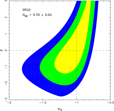
Figure 1: Probability contours from the SNLS data only at 68.3%, 95.4% and 99.7% confidence levels in the ($w_{X},\delta$) plane marginalized over $\Omega_{X0}$ with priors $\Omega_{X0}=0.72\pm 0.04$ and $\delta<3$ in the constant coupling models. The horizontal and dashed lines represent the uncoupled “XCDM” models and the coupled $\Lambda$CDM models respectively, and their crossing point corresponds to the standard $\Lambda$CDM model. In this case we have the constraint $-1.78<\delta<3$ (95% CL).

In this plane, the horizontal dashed line represents the uncoupled models with $\delta=0$ and the vertical dashed line represents the coupled $\Lambda$CDM models with $w_{X}=-1$.

II.2 Varying coupling models

When $\delta$ varies in time, Eq. (2) together with Eq. (4) gives

$$\rho_{m}=\rho_{m0}a^{-3}e^{\int\delta\;{\rm d}(\ln a)}\,.$$ (9)

Let us now consider a situation in which the ratio of dark energy and dark matter has the following relation dal01 :

$$\frac{\rho_{X}}{\rho_{m}}=\frac{\rho_{X0}}{\rho_{m0}}a^{\xi},$$ (10)

where $\xi$ is a constant which quantifies the severity of the coincidence problem. In the absence of the coupling $\delta$ with constant $w_{X}$, the energy density of dark energy scales as $\rho_{X}\propto a^{-3(1+w_{X})}$. Here the ratio $\rho_{X}/\rho_{m}$ is proportional to $a^{-3w_{X}}$, namely, the $\xi=-3w_{X}$ case in Eq. (10). Note that the standard $\Lambda$CDM model corresponds to $w_{X}=-1$ and $\xi=3$.

The general case $\xi\neq-3w_{X}$ indicates the existence of an interaction between dark matter and dark energy. Using the relation (10), we find that the coupling $\Gamma$ is given by $\Gamma=-H(\xi+3w_{X})\Omega_{X}(z)$, where $\Omega_{X}(z)=\kappa^{2}\rho_{X}/(3H^{2})$. This shows that $\delta$ varies according to the change of $\Omega_{X}$ as

$$\delta(z)=-(\xi+3w_{X})\Omega_{X}(z)\,.$$ (11)

When $\xi=-3w_{X}$, this reduces to $\delta=0$. Since $\Omega_{X}(z)$ is given by $\Omega_{X}(z)=\left[(\rho_{m0}/\rho_{X0})(1+z)^{\xi}+1\right]^{-1}$ under the condition (10), the coupling can be written as

$$\delta(z)=\frac{\delta_{0}}{\Omega_{X0}+(1-\Omega_{X0})(1+z)^{\xi}}\,,$$ (12)

where $\delta_{0}=-(\xi+3w_{X})\Omega_{X0}$. If $\xi>0$, $\delta(z)$ decreases for higher $z$.

Note that the $\xi=0$ case gives a constant coupling $\delta(z)=\delta_{0}$. Since this corresponds to an exact scaling solution $\rho_{X}\propto\rho_{m}$, one cannot realize the matter dominated epoch followed by a late-time acceleration. This constant $\delta$ case is different from the one we discussed in subsection A. In fact the solutions (6) and (II.1) do not satisfy the relation (10).

From Eqs. (2) and (3) together with Eq. (10), the total energy density $\rho_{T}=\rho_{m}+\rho_{X}$ satisfies

$$\frac{{\rm d}\ln\rho_{T}}{{\rm d}a}=-\frac{3}{a}\left[1+w_{X}\left(\frac{\rho_{m0}}{\rho_{X0}}a^{-\xi}+1\right)^{-1}\right]\,,$$ (13)

which can be integrated to give

$$\rho_{T}=\rho_{T0}\,a^{-3}\left[1-\frac{\rho_{X0}}{\rho_{T0}}(1-a^{\xi})\right]^{-3w_{X}/\xi}\,.$$ (14)

Then the Friedmann equation (5) gives

$$E^{2}(z)=(1+z)^{3}\left[1-\Omega_{X0}+\Omega_{X0}(1+z)^{-\xi}\right]^{-3w_{X}/\xi}\,.$$ (15)

From Eq. (10), we find that the energy density of dark energy is given by

$$\rho_{X}=\rho_{T}\frac{\Omega_{X0}}{\Omega_{X0}+(1-\Omega_{X0})(1+z)^{\xi}}\,.$$ (16)

We have three parameters ($\xi$, $w_{X}$, $\Omega_{X0}$) in this model. Since $\delta_{0}$ is related to these variables by the relation $\delta_{0}=-(\xi+3w_{X})\Omega_{X0}$, one can instead vary three parameters ($\delta_{0}$, $w_{X}$, $\Omega_{X0}$) when we carry out likelihood analysis. Thus the model (15) is a simple parametrization that implements the variation of the coupling $\delta$. Note that both $\rho_{T}$ and $\rho_{X}$ are positive as long as $0<\Omega_{X0}<1$. Hence $\rho_{X}$ remains positive in the high-redshift region even for $\delta<0$ unlike the constant coupling model.

The coupling affects the evolution of some quantities of interest, such as the age of the universe and the deceleration parameter. Given $w_{X}$ and $\Omega_{X0}$, the age of the universe and the transition redshift at which the universe switches from deceleration to acceleration become larger as the value of $\delta_{0}$ increases from negative to positive. In the next section, we place observational constraints on the strength of the coupling.

III Constraints from Recent Observations

In this section, we study the viability of interacting models presented in the previous section by using recently released SNLS data ast05 in conjunction with the BAO peak in the SDSS eis05 and the CMB shift parameter wan06 .

Recently Astier et al. ast05 have compiled a new sample of 71 high-redshift SNe Ia, in the redshift range $0.2<z<1.0$, discovered during the first year of the 5-year SNLS. This data set is arguably the best high-redshift SN Ia compiled data, since the multi-band, rolling search technique and careful calibration are adopted. The luminosity distance $d_{L}(z)$ to supernovae is given by review ; CST

$$d_{L}(z)=H_{0}^{-1}(1+z)\int_{0}^{z}\frac{{\rm d}z^{\prime}}{E(z^{\prime})}\,.$$ (17)

The baryon oscillations in the galaxy power spectrum are imprints from acoustic oscillations prior to recombination, which are also responsible for the acoustic peaks seen in the CMB temperature power spectrum. The physical length scale associated with the oscillations is set by the sound horizon at recombination, which can be estimated from the CMB data spe06 . Measuring the apparent size of the oscillations in a galaxy survey allows one to measure the angular diameter distance at the survey redshift. Although the acoustic features in the matter correlations are weak on large scales, Eisenstein et al. eis05 have successfully found the peaks using a large spectroscopic sample of luminous red galaxies from SDSS yor00 . This sample contains 46,748 galaxies covering 3816 square degrees out to a redshift of $z=0.47$. They found a parameter $A$, which is independent of dark energy models eis05 . From Eq. (5) in their paper eis05 , we write it as

$$A=\sqrt{\Omega_{m0}}\,E(z_{1})^{-1/3}\left[\frac{1}{z_{1}}\int_{0}^{z_{1}}\frac{{\rm d}z^{\prime}}{E(z^{\prime})}\right]^{2/3},$$ (18)

where $z_{1}=0.35$ and $A$ is measured to be $A=0.469\pm 0.017$. In our analysis, we combine these measurements.

The CMB shift parameter $\cal{R}$ captures the correspondence between the angular diameter distance to last scattering surface and the relation of the angular scale of the acoustic peaks to the physical scale of the sound horizon bon97 . Its value is expected to be mostly model-independent, which can be extracted accurately from CMB data. The shift parameter $\cal{R}$ is given by wan04

$${\cal R}=\sqrt{\Omega_{m0}}\int_{0}^{z_{{\rm rec}}}\frac{{\rm d}z^{\prime}}{E(z^{\prime})}\,,$$ (19)

where $z_{\rm rec}$ is the redshift of recombination. It provides a useful constraint on evolving dark energy models since the integral over $E(z)$ extends to high redshifts. The recent analysis of the three-year WMAP data spe06 gives ${\cal R}=1.70\pm 0.03$ at $z_{\rm rec}=1089$ wan06 .

III.1 Constant coupling models

Let us first consider observational constraints on constant coupling models. In Fig. 1, we show probability contours from SNLS when we take a prior for $\Omega_{X0}$ such that the probability distribution is a Gaussian with a mean of $0.72$ and a standard deviation given by $\sigma=0.04$. We also assume the condition $\delta<3$ to exclude the possibility that dark matter behaves as a phantom matter [see Eq. (6)]. The phantom dark matter is problematic for successful structure formation. Then we find that the SNLS data gives a weak constraint on the coupling as $-1.78<\delta<3$ at the 95% confidence level. When we choose the wider range of the prior for $\Omega_{X0}$, the constraint becomes weaker.

Figure 2 shows the case in which the BAO data is taken into account in addition to the SNLS data without a prior for $\Omega_{X0}$. Compared to Fig. 1, the allowed range of $w_{X}$ is reduced. However we still have a rather large region of a parameter space for $\delta$, i.e., $-1.73<\delta<3$ (95% CL).

We have also carried out a likelihood analysis without any prior for $\delta$ and found that even the large coupling such as $\delta=20$ with $w_{X}\sim-0.7$ is within the $2\sigma$ observational contour bound. This reflects the fact that the SNIa and BAO data give constraints only around low redshifts $z<{\cal O}(1)$. The models can fit the data even for $\delta\gg 1$ because of the dominance of the $\delta(1+z)^{3(1+w_{X})}$ term instead of the usual $3w_{X}(1+z)^{3-\delta}$ term on the rhs of Eq. (LABEL:model1). This tells us how it is important to include other data in a high-redshift region ($z\gg 1$) in order to rule out models with problematic couplings ($\delta>3$).

In fact the CMB shift parameter provides a stringent constraint on the coupling. In Fig. 3 we plot observational contours from the joint analysis of SNLS, CMB and BAO data in the ($w_{X},\delta$) plane marginalized over $\Omega_{X0}$ (left panel) and in the ($\Omega_{X0},\delta$) plane marginalized over $w_{X}$ (right panel). Note that we do not put any prior for $\delta$ in these analysis. We find that the coupling is severely constrained: $-0.08<\delta<0.03$ (95% CL) in both marginalizations. This comes from the fact that the CMB data do not allow a large deviation from the standard matter-dominated epoch.

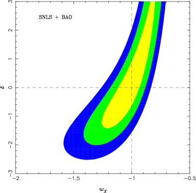
Figure 2: Probability contours from the SNLS and BAO data in the ($w_{X},\delta$) plane marginalized over $\Omega_{X0}$ without a prior for $\Omega_{X0}$ and with a prior $\delta<3$ in the constant coupling models. In this case we have the constraint $-1.73<\delta<3$ (95% CL).

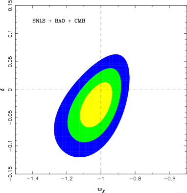
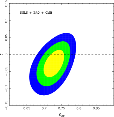
Figure 3: Probability contours from the combination of SNLS, BAO and CMB data in the constant coupling models. The left panel shows observational contours in the ($w_{X},\delta$) plane marginalized over $\Omega_{X0}$ without a prior for $\Omega_{X0}$, whereas the right panel shows contours in the ($\Omega_{X0},\delta$) plane marginalized over $w_{X}$ with no prior for $w_{X}$. The best-fit model parameters correspond to $\delta=-0.03$, $w_{X}=-1.02$ and $\Omega_{X0}=0.73$ with $\chi^{2}=60.94$. In this case we have the constraint $-0.08<\delta<0.03$ (95% CL).

The combined analysis of three databases constrains the equation of state and the present energy fraction of dark energy to $-1.16<w_{X}<-0.91$ and $0.69<\Omega_{X0}<0.77$ (95% CL). It is interesting to note that the allowed observational contours are widely spread in the phantom region ($w_{X}<-1$) with a negative coupling ($\delta<0$), see Fig. 3. The best-fit parameters are found to be $\delta=-0.03$, $w_{X}=-1.02$ and $\Omega_{X0}=0.73$ with $\chi^{2}=60.94$, which is slightly favoured over the $\Lambda$CDM model.

III.2 Varying coupling models

We now proceed to the varying coupling models in which $\delta$ depends upon $z$ in the form (12). In Fig. 4 we show observational contours from the combined analysis of SNLS$+$BAO$+$CMB data in the planes (i) $(w_{X},\delta_{0})$ marginalized over $\Omega_{X0}$ (left panel) and (ii) $(\Omega_{X0},\delta_{0})$ marginalized over $w_{X}$ (right panel). We find that the present coupling, the dark energy equation of state and the present dark energy density are constrained to be $-0.4<\delta_{0}<0.1$, $-1.18<w_{X}<-0.91$ and $0.69<\Omega_{X0}<0.77$ at the 95% confidence level. The best-fit parameters correspond to $\delta=-0.11$, $w_{X}=-1.03$ and $\Omega_{X0}=0.73$ with $\chi^{2}=60.94$. Similarly to the constant coupling case, the SNIa and BAO data do not provide stringent constraints on $\delta_{0}$, but inclusion of the CMB data significantly reduces the allowed region of the coupling. Since $\delta(z)$ decreases for larger $z$, the observational constraints on $\delta_{0}$ is not so severe compared to the constant coupling models. We also find that the phantom models ($w_{X}<-1$) with a negative coupling ($\delta_{0}<0$) have a wider allowed parameter space compared to three other divided regions in the left panel of Fig. 4.

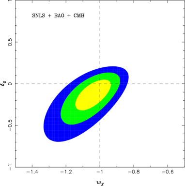
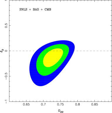
Figure 4: Probability contours from the joint analysis of the SNLS, BAO and CMB data in the varying coupling models. The left panel shows observational contours in the $(w_{X},\delta_{0})$ plane marginalized over $\Omega_{X0}$ without prior for $\Omega_{X0}$, whereas the right panel shows contours in the ($\Omega_{X0},\delta$) plane marginalized over $w_{X}$ without prior for $w_{X}$. The best-fit parameters correspond to $\delta=-0.11$, $w_{X}=-1.03$ and $\Omega_{X0}=0.73$ with $\chi^{2}=60.94$. In this case we have the constraint $-0.4<\delta_{0}<0.1$ (95% CL).

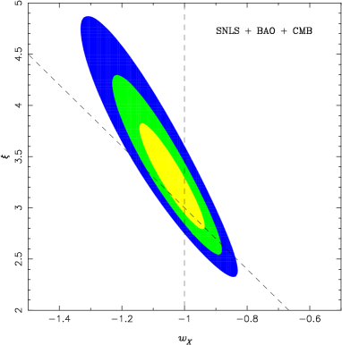
Figure 5: Probability contours in the varying coupling models in the $(w_{X},\xi)$ plane marginalized over $\Omega_{X0}$. The line $\xi=-3w_{X}$ corresponds to the uncoupled models. In this case we have the constraint $2.66<\xi<4.05$ (95% CL).

As we see from Fig. 5, the $\Lambda$CDM model, which corresponds to the point $(w_{X},\xi)=(-1,3)$, is within the 1$\sigma$ contour bound. We remind that the uncoupled models are characterized by the line $\xi=-3w_{X}$. Thus, provided that the points are not on the line $\xi=-3w_{X}$, the coupled models are allowed observationally in the parameter regions $2.66<\xi<4.05$ (95% CL). From Fig. 5 it is obvious that the scaling models with $\xi=0$ are excluded from the data.

IV Conclusions

In this paper, we have studied interacting models of dark energy in which the coupling $\delta$ between dark matter and dark energy is given by (4) together with conservation equations (2) and (3). We discussed two different models: (i) constant $\delta$ case, and (ii) varying $\delta$ case which has a redshift dependence given in (12). The latter type of couplings appears by imposing the relation $\rho_{X}/\rho_{m}\propto a^{\xi}$ between the energy densities of two dark components. Assuming that the equation of state of dark energy $w_{X}$ is a constant, we obtain the convenient forms of the Friedmann equations (LABEL:model1) and (15) to confront with observational data.

We have placed observational constraints on the strength of the coupling $\delta$ by using the recent data of SNLS, the CMB shift parameter and the SDSS baryon acoustic oscillations (BAO). In both constant and varying coupling models, the supernova data alone do not provide stringent constraints on the coupling. Adding the BAO data generally reduces the allowed range of $w_{X}$, but the coupling $\delta$ of order unity is not still ruled out. This reflects the fact that the BAO and SN Ia data are sensitive to the value of $w_{X}$ or $\Omega_{X0}$ rather than $\delta$. However the combined analysis of SNLS$+$BAO$+$CMB shows that the allowed region of the coupling is significantly reduced compared to the case without the CMB data. This is associated with the fact that a large coupling leads to the change of the cosmological evolution during the matter-dominated epoch, thus modifying the CMB angular-diameter distance.

By the joint analysis of SNLS$+$BAO$+$CMB, we have obtained observational constraints on the strength of the coupling: (i) $-0.08<\delta<0.03$ (95% CL) for the constant coupling models and (ii) $-0.4<\delta_{0}<0.1$ (95% CL) for the varying coupling models (here $\delta_{0}$ is a present value). We also find that the best-fit values exist in the phantom region ($w_{X}<-1$) with a negative coupling ($\delta<0$) in both constant and varying coupling models. The uncoupled $\Lambda$CDM model ($w_{X}=-1$ and $\delta=0$) still remains a good fit to the data. Nevertheless it is interesting to note that the negative coupling with a dark energy with $w_{X}<-1$ is slightly favoured over the $\Lambda$CDM model.

There exist coupled dark energy models Huey ; das05 that give $w_{X}<-1$ without using a negative kinetic energy of a scalar field (called “super-acceleration” in Ref. das05 ). This can be realized by considering scalar-field dependent masses of dark matter particles. It was shown in Ref. das05 that this super-acceleration model satisfies a number of observational constraints, which is consistent with our results that the equation of state $w_{X}<-1$ is favoured.

In this work we did not take into account observational constraints from matter density perturbations $\delta_{m}$ which is also affected by the presence of the coupling mper . It was shown in Ref. Fabris that the inclusion of matter density perturbations can place a stronger constraint on the coupling $\delta$ compared to the analysis using the background evolution only. The future galaxy surveys such as KAOS and PANSTARS will further provide good data of the matter power spectrum with a high accuracy, which can offer a possibility to put severe constraints on the coupling. This may provide us an exciting possibility to reveal the origin of dark energy and dark matter.

References

- (1) A. G. Riess et al., Astron. J. 116, 1009 (1998); Astron. J. 117, 707 (1999).
- (2) S. Perlmutter et al., Astrophys. J. 517, 565 (1999).
- (3) P. Astier et al., Astron. Astrophys. 447, 31 (2006)
- (4) D. N. Spergel et al. [WMAP Collaboration], Astrophys. J. Suppl. 148, 175 (2003).
- (5) D. N. Spergel et al., arXiv:astro-ph/0603449.
- (6) D. J. Eisenstein et al. [SDSS Collaboration], Astrophys. J. 633, 560 (2005).
- (7) V. Sahni and A. A. Starobinsky, Int. J. Mod. Phys. D 9, 373 (2000); V. Sahni, Lect. Notes Phys. 653, 141 (2004); S. M. Carroll, Living Rev. Rel. 4, 1 (2001); T. Padmanabhan, Phys. Rept. 380, 235 (2003); P. J. E. Peebles and B. Ratra, Rev. Mod. Phys. 75, 559 (2003).
- (8) E. J. Copeland, M. Sami and S. Tsujikawa, Int. J. Mod. Phys. D 15, 1753 (2006).
- (9) R. R. Caldwell, R. Dave and P. J. Steinhardt, Phys. Rev. Lett. 80, 1582 (1998); I. Zlatev, L. M. Wang and P. J. Steinhardt, Phys. Rev. Lett. 82, 896 (1999).
- (10) Y. Fujii, Phys. Rev. D 26, 2580 (1982); L. H. Ford, Phys. Rev. D 35, 2339 (1987); C. Wetterich, Nucl. Phys B. 302, 668 (1988); B. Ratra and J. Peebles, Phys. Rev D 37, 321 (1988); Y. Fujii and T. Nishioka, Phys. Rev. D 42, 361 (1990).
- (11) A. A. Starobinsky, JETP Lett. 68, 757 (1998); D. Huterer and M. S. Turner, Phys. Rev. D 60, 081301 (1999); T. Chiba and T. Nakamura, Phys. Rev. D 62, 121301 (2000); M. Sahlen, A. R. Liddle and D. Parkinson, Phys. Rev. D 72, 083511 (2005); Z. K. Guo, N. Ohta and Y. Z. Zhang, Phys. Rev. D 72, 023504 (2005); S. Tsujikawa, Phys. Rev. D 72, 083512 (2005); Z. K. Guo, N. Ohta and Y. Z. Zhang, Mod. Phys. Lett. A 22, 883 (2007).
- (12) J. Ellis, S. Kalara, K. A. Olive and C. Wetterich, Phys. Lett. B 228, 264 (1989); T. Damour and K. Nordtvedt, Phys. Rev. D 48, 3436 (1993); T. Damour and A. M. Polyakov, Nucl. Phys. B 423, 532 (1994).
- (13) L. Amendola, Phys. Rev. D62, 043511 (2000).
- (14) L. Amendola, Phys. Rev. D 60, 043501 (1999).
- (15) L. Amendola, D. Polarski and S. Tsujikawa, Phys. Rev. Lett. 98, 131302 (2007).
- (16) M. Doran and J. Jaeckel, Phys. Rev. D 66, 043519 (2002); D. Comelli, M. Pietroni and A. Riotto, Phys. Lett. B 571, 115 (2003); H. Ziaeepour, Phys. Rev. D 69, 063512 (2004); M. Axenides and K. Dimopoulos, JCAP 0407 (2004) 010.
- (17) G. Huey and B. D. Wandelt, Phys. Rev. D 74, 023519 (2006).
- (18) S. Das, P. S. Corasaniti and J. Khoury, Phys. Rev. D 73, 083509 (2006).
- (19) P. Q. Hung, arXiv:hep-ph/0010126; M. Li, X. Wang, B. Feng and X. Zhang, Phys. Rev. D 65, 103511 (2002); M. Li and X. Zhang, Phys.Lett. B 573, 20 (2003); R. Fardon, A. E. Nelson and N. Weiner, JCAP 0410, 005 (2004); H. Li, B. Feng, J. Q. Xia and X. Zhang, Phys. Rev. D 73, 103503 (2006); A. W. Brookfield, C. van de Bruck, D. F. Mota and D. Tocchini-Valentini, Phys. Rev. Lett. 96, 061301 (2006); Phys. Rev. D 73, 083515 (2006).
- (20) Z. K. Guo and Y. Z. Zhang, Phys. Rev. D 71, 023501 (2005); R. G. Cai and A. Wang, JCAP 0503, 002 (2005); Z. K. Guo, R. G. Cai and Y. Z. Zhang, JCAP 0505, 002 (2005); R. Curbelo, T. Gonzalez and I. Quiros, Class. Quant. Grav. 23, 1585 (2006); B. Chang et al., JCAP 01, 016 (2007).
- (21) B. Gumjudpai, T. Naskar, M. Sami and S. Tsujikawa, JCAP 0506, 007 (2005).
- (22) F. Piazza and S. Tsujikawa, JCAP 0407, 004 (2004); S. Tsujikawa and M. Sami, Phys. Lett. B 603, 113 (2004).
- (23) L. Amendola, M. Quartin, S. Tsujikawa and I. Waga, Phys. Rev. D 74, 023525 (2006).
- (24) L. Amendola and D. Tocchini-Valentini, Phys. Rev. D 64, 043509 (2001).
- (25) N. Dalal, K. Abazajian, E. Jenkins and A. V. Manohar, Phys. Rev. Lett. 87, 141302 (2001).
- (26) W. Zimdahl, D. Pavon and L. P. Chimento, Phys. Lett. B521 (2001) 133; W. Zimdahl and D. Pavon, Gen. Rel. Grav. 35, 413 (2003); L. P. Chimento, A. S. Jakubi, D. Pavon and W. Zimdahl, Phys. Rev. D 67, 083513 (2003).
- (27) E. Majerotto, D. Sapone and L. Amendola, arXiv:astro-ph/0410543.
- (28) H. Wei and S. N. Zhang, Phys. Lett. B 644, 7 (2007).
- (29) L. Amendola, G. Camargo Campos and R. Rosenfeld, Phys. Rev. D 75, 083506 (2007).
- (30) D. Pavon, S. Sen and W. Zimdahl, JCAP 0405, 009 (2004); G. Olivares, F. Atrio-Barandela and D. Pavon, Phys. Rev. D 71, 063523 (2005); Phys. Rev. D 74, 043521 (2006); S. del Campo, R. Herrera, G. Olivares and D. Pavon, Phys. Rev. D 74, 023501 (2006).
- (31) U. Franca and R. Rosenfeld, Phys. Rev. D 69, 063517 (2004).
- (32) A. V. Maccio et al., Phys. Rev. D 69, 123516 (2004).
- (33) M. Nishiyama, M. a. Morita and M. Morikawa, arXiv:astro-ph/0403571.
- (34) S. Nojiri, S. D. Odintsov and S. Tsujikawa, Phys. Rev. D 71, 063004 (2005); S. Nojiri and S. D. Odintsov, Phys. Rev. D 72, 023003 (2005); Gen. Rel. Grav. 38, 1285 (2006).
- (35) G. Calcagni, S. Tsujikawa and M. Sami, Class. Quant. Grav. 22, 3977 (2005); S. Tsujikawa, Phys. Rev. D 73, 103504 (2006).
- (36) S. Das and N. Banerjee, Gen. Rel. Grav. 38, 785 (2006).
- (37) H. Wei and R. G. Cai, Phys. Rev. D 71, 043504 (2005); Phys. Rev. D 73, 083002 (2006); H. Zhang and Z. H. Zhu, Phys. Rev. D 73 043518 (2006); H. Wei and R. G. Cai, arXiv:astro-ph/0607064.
- (38) X. Zhang, Phys. Lett. B 611, 1 (2005); Mod. Phys. Lett. A 20, 2575 (2005).
- (39) B. Wang, Y. g. Gong and E. Abdalla, Phys. Lett. B 624, 141 (2005); D. Pavon and W. Zimdahl, Phys. Lett. B 628 206 (2005); B. Wang, C. Y. Lin and E. Abdalla, Phys. Lett. B 637, 357 (2006); H. Li, Z. K. Guo and Y. Z. Zhang, Int. J. Mod. Phys. D 15, 869 (2006).
- (40) T. Koivisto, Phys. Rev. D 72, 043516 (2005).
- (41) D. F. Mota and D. J. Shaw, Phys. Rev. Lett. 97, 151102 (2006).
- (42) Z. G. Huang, H. Q. Lu and W. Fang, Class. Quant. Grav. 23, 6215 (2006); arXiv:hep-th/0610018.
- (43) B. Hu and Y. Ling, Phys. Rev. D 73, 123510 (2006).
- (44) S. Lee, G. C. Liu and K. W. Ng, Phys. Rev. D 73, 083516 (2006).
- (45) N. J. Poplawski, Phys. Rev. D 74, 084032 (2006).
- (46) H. M. Sadjadi and M. Alimohammadi, Phys. Rev. D 74, 103007 (2006); H. M. Sadjadi and M. Honardoost, Phys. Lett. B 647, 231 (2007).
- (47) S. A. Bonometto, L. Casarini, L. P. L. Colombo and R. Mainini, arXiv:astro-ph/0612672.
- (48) N. Tetradis, J. D. Vergados and A. Faessler, Phys. Rev. D 75, 023504 (2007).
- (49) R. Rosenfeld, Phys. Rev. D 75, 083509 (2007).
- (50) M. R. Setare, Phys. Lett. B 642, 1 (2006); Phys. Lett. B 642, 421 (2006); JCAP 01, 023 (2007); arXiv:hep-th/0701085.
- (51) R. Bean and J. Magueijo, Phys. Lett. B 517, 177 (2001); R. Bean, Phys. Rev. D 64 123516 (2001).
- (52) M. Szydlowski, Phys. Lett. B 632, 1 (2006); M. Szydlowski, T. Stachowiak and R. Wojtak, Phys. Rev. D 73, 063516 (2006).
- (53) M. Manera and D. F. Mota, Mon. Not. Roy. Astron. Soc. 371, 1373 (2006); A. Arbey, Phys. Rev. D 74, 043516 (2006); A. Arbey, arXiv:astro-ph/0506732; M. C. Bento et al., Phys. Rev. D 73, 103521 (2006); M. C. Bento et al., Phys. Rev. D 73, 043504 (2006).
- (54) R. R. Caldwell, Phys. Lett. B 545, 23 (2002).
- (55) L. Amendola, R. Gannouji, D. Polarski and S. Tsujikawa, Phys. Rev. D 75, 083504 (2007).
- (56) Y. Wang and P. Mukherjee, Astrophys. J. 650, 1 (2006).
- (57) D. G. York et al., Astron. J. 120, 1579 (2000).
- (58) J. R. Bond, G. Efstathiou and M. Tegmark, Mon. Not. Roy. Astron. Soc. 291, L33 (1997).
- (59) Y. Wang and P. Mukherjee, Astrophys. J. 606, 654 (2004).
- (60) L. Amendola, Phys. Rev. D 69, 103524 (2004); L. Amendola, S. Tsujikawa and M. Sami, Phys. Lett. B 632, 155 (2006).
- (61) J. C. Fabris, I. L. Shapiro and J. Sola, JCAP 0702, 016 (2007).