Variable VHE $\gamma$-ray emission from Markarian 501

Abstract

The blazar Markarian 501 (Mrk 501) was observed at energies above 0.10 TeV with the MAGIC telescope from May through July 2005. The high sensitivity of the instrument enabled the determination of the flux and spectrum of the source on a night-by-night basis. Throughout our observational campaign, the flux from Mrk 501 was found to vary by an order of magnitude. Intra-night flux variability with flux-doubling times down to 2 minutes was observed during the two most active nights, namely June 30 and July 9. These are the fastest flux variations ever observed in Mrk 501. The $\sim$20-minute long flare of July 9 showed an indication of a 4$\pm$1 min time delay between the peaks of F($<$0.25 TeV) and F($>$1.2 TeV), which may indicate a progressive acceleration of electrons in the emitting plasma blob. The flux variability was quantified for several energy ranges, and found to increase with the energy of the $\gamma$-ray photons. The spectra hardened significantly with increasing flux, and during the two most active nights, a spectral peak was clearly detected at 0.43 $\pm$ 0.06 TeV and 0.25 $\pm$ 0.07 TeV, respectively for June 30 and July 9. There is no evidence of such spectral feature for the other nights at energies down to 0.10 TeV, thus suggesting that the spectral peak is correlated with the source luminosity. These observed characteristics could be accommodated in a Synchrotron-Self-Compton (SSC) framework in which the increase in $\gamma$-ray flux is produced by a freshly injected (high energy) electron population.

1 Introduction

The large inferred luminosities of Active Galactic Nuclei (AGNs) led to a standard model of beamed AGN emission, with the ultimate energy source being the release of gravitational potential energy of matter from an accretion disk surrounding a super-massive black hole (Rees, 1984). Particularly interesting for the Very-High-Energy $\gamma$-ray (VHE) community are the blazars, whose relativistic plasma jets point at the observer. Distinctive features of blazars are their continuum emission, clearly non-thermal from radio to VHE frequencies and characterized by two broad bumps peaking at, respectively, IR/X-ray and $\gamma$-ray frequencies (Blandford & Rees, 1978; Urry & Padovani, 1995; Ulrich et al, 1997), and their strong variability, implying flux variations by a factor of $\sim$$>$ 10 over timescales of $\sim$$<$ 1 hour to months (flares; see Ulrich et al. 1997).

So far, 13 AGNs have been detected at VHE energies. Except for M87 (Aharonian et al, 2003, 2006), all these sources belong to the ’high-peaked BL Lac’ (HBL) sub-class of blazars, which are characterized by a spectral energy density (SED) in which both maxima occur at relatively high frequency (e.g., respectively at hard X-rays and HE/VHE $\gamma$-rays). The detection of $\gamma$-rays from blazars leads to some important considerations about the relevant radiation processes and the physical properties of the emitting regions. Most notably, the very detection of VHE radiation, implying $\gamma$-ray transparency in the emitting region, requires the presence of relativistic beaming to decrease the intrinsic energy density of the soft target photons inside the source. The beaming reduces this value because it simultaneously decreases the intrinsic energy density of the photons and, having reduced the energy of the relevant $\gamma$-ray photons, it increases the energy of the soft target photons relevant to e^± production, hence (for typical spectra) decreasing their number density (McBreen 1979; (Blandford & Königl, 1979). Bassani & Dean 1981; (Mattox et al, 1993); Dondi & Ghisellini 1995).

Two classes of emission models have been proposed to explain the TeV emission from blazars: leptonic and hadronic models.
(i) In the case of the most popular leptonic models, the same population of non-thermal electrons (and possibly positrons) responsible for the radio-to-X-rays SED is also responsible for $\gamma$-ray  emission, through Compton up-scattering of the synchrotron photons off their own parent electrons – the Synchrotron-Self-Compton (SSC) process (Marscher et al, 1985; Maraschi et al, 1992; Böttcher, 2002). In other models, electrons scatter ’external’ photons that originate outside the jet (External Compton (EC) models). In BL Lacs the lack of strong emission lines suggests a minor role of ambient photons and hence supports the SSC models.
(ii) In hadronic models, the TeV radiation is produced by hadronic interactions of the highly relativistic baryonic outflow with the ambient medium, and/or by interactions of ultra-high-energy protons with synchrotron photons produced by electrons (Mannheim & Biermann, 1992), with the jet magnetic field (Aharonian et al, 2000), or with both (Mücke et al, 2003; Atoyan et al, 2003; Mannheim, 1993).
However, hadronic models are challenged by the blazars’ observed X-ray versus VHE correlation and very rapid $\gamma$-ray variability. The SSC model is then widely believed to explain the dominant emission process in blazar jets (not always in its simplest one-zone realization, as required by e.g. ’orphan flares’: see Krawczynski et al (2004) and Gliozzi et al (2006)).

In this framework, the importance of high-quality data on blazar VHE emission can not be overestimated. In particular, valuable information can be obtained investigating: (i) the rapid, possibly energy-dependent, flux variability; (ii) the X-ray/optical versus VHE correlation; and (iii) the X-ray and VHE spectral variability, with a potential energy shift of the Synchrotron and Compton peaks. Simultaneous multi-wavelength observations of such rapid variability can provide stringent tests to emission models, in particular on acceleration processes in jets. In the case of nearby ($z$$<$0.1) sources, the extinction due to pair production by interaction of the blazar-emitted TeV photons with the (not well known) optical/IR Extragalactic Background Light (EBL) photons is probably minor, and thus there is a smaller uncertainty in the determination of the intrinsic spectral features of the object.

In this paper we report about detailed measurements of the VHE emission of Mrk 501, demonstrating the capability of the MAGIC Telescope in the precision study of blazar physics. The BL Lac object Mrk 501 was the second established TeV-blazar (Quinn et al, 1996; Bradbury et al, 1997). After a phase of moderate emission for about a year following its discovery as a TeV source, in 1997 Mrk 501 went into a state of surprisingly high activity and strong variability, becoming $>$10 times brighter (at energies $>$1 TeV) than the Crab Nebula (Aharonian et al, 1999a, b). In 1998-1999 the mean flux dropped by an order of magnitude (Aharonian et al, 2001). It is worth noticing that the HEGRA observations (with a threshold energy of $\sim$0.5 TeV) did not see spectral variations during the 1997 outburst, whereas it did observe in 1998-1999 a significantly softer low-state energy spectrum than in 1997. The CAT telescope (with a threshold energy of  0.25 TeV), on the other hand, did detect spectral variations during 1997 (Djanati-Ataïet al, 1999; Piron, 2000, 2001).

The structure of the paper is as follows. In sect. 2 we briefly describe the MAGIC data taking and analysis. In sects. 3 and 4 we present and discuss the Mrk 501 VHE lightcurve (hereafter LC), spectrum and their variability, during the observation campaign. In sect.5 we discuss the long-term light curve of Mrk 501, short-term flux variability, flux-spectrum correlations, and the overall SED of this object. Finally, sect. 6 summarizes our main results.

2 The MAGIC Telescope and the data analysis

2.1 The instruments

The observations in the VHE domain were carried out with the Major Atmospheric Gamma-ray Imaging Cherenkov (MAGIC) telescope, located on the Canary island of La Palma (28.8^o$N$, 17.9^o$W$) at the Roque de los Muchachos Observatory (about 2200 m above see level). MAGIC started regular observations in the fall of 2004 and, with a main mirror diameter of 17 m, it is currently the world’s largest single-dish IACT. Further details about the characteristics and performance of MAGIC can be found elsewhere (Baixeras et al, 2004; Paneque, 2004; Cortina et al, 2005; Gaug, 2006).

The MAGIC Collaboration also operates the optical KVA telescope (35 cm). Simultaneously with the MAGIC observations, Mrk 501 was regularly observed with KVA as a part of the Tuorla Observatory blazar monitoring program. In this paper we also use 2-10 keV data taken with the RXTE satellite’s All-Sky-Monitor (RXTE/ASM) quasi-simultaneously with our MAGICobservations.

2.2 Source observation

The source was observed during 30 nights between May and July 2005, with an overall observation time of 54.8 hours. In order to maximize the time coverage of this source, observations were carried out also in the presence of moonlight (34.1 hours, i.e. 62% of the total observing time). It is important to note that many of these ’moon observations’ were performed when the moon was only partly illuminated, and mostly located at a large angle (60^o-90^o) with respect to the position of Mrk 501. This kept the Night Sky Background (NSB) of these observations rather low and comparable to that of the moonless observations. The observations were mostly performed in the so-called ’on mode’ in which the telescope points exactly to the source (on-data), and thus its (optical) image is right in the center of the camera. The telescope was also operated in ’off mode’, in which it points to regions of the sky where there are no known $\gamma$-ray sources (off-data). These observations were carried out at comparable zenith angle (ZA) and NSB conditions, and can therefore be used to estimate the background content of the on-data. The off-data observation time amounts to 3.5 hours.

The data were screened for hardware problems, non-optimal weather conditions, and too high NSB light. In addition, the very few runs with ZA larger than 30^o that survived those filters were also removed, in order to have a more uniform data set. The number of nights surviving these selection cuts is 24, with a total net observation time of 31.6 hours. These observation nights, together with the corresponding net times and ZA ranges of the data acquisition, are listed in Table 1.

2.3 Data analysis

The analysis used in this paper is based on the Hillas image parameters ALPHA, WIDTH, LENGTH, DIST and SIZE to quantify the camera image, see Hillas (1985). These parameters are calculated using the calibrated signals from the individual pixels of the camera. The procedures used to calibrate the PMT signals in MAGIC are described in detail in Gaug (2006) and Albert et al (2006): here we used the Sliding Window signal extractor, and performed the calibration with the Excess Noise Factor method. Only PMT signals with more than 10 photoelectrons (8 photoelectrons for pixels in the boundary of an image) which occur within a time window of 6.6 ns (2 FADC slices) of the neighbouring pixel signal were used. The minimum total image light content (SIZE) considered in this analysis is 150 photelectrons. The signal/background separation is achieved by applying dynamical cuts (defined as 2nd order polynomial functions of logSIZE) on the parameters WIDTH, LENGTH (shape parameters) and DIST (position of the image). The background contained in the on-data after the $\gamma$/hadron separation cuts is estimated by means of a 2nd-order polynomial fit (with no linear term) to the ALPHA distribution from the normalized (according to the on-off observation times) off-data.

The energy of the incoming $\gamma$-rays is essentially proportional to the light content of the image (SIZE), with corrections according to the values of LENGTH, DIST and LEAKAGE. The energy resolution achieved with this parameterization is about 20-30%, slightly depending on the event’s energy. Because of the finite experimental resolution, the distribution of the excess events ($\gamma$-candidates) versus the reconstructed energy is a convolution of the (true) energy distribution of excess events and a realistic energy resolution function. The determination of the true energy spectrum from the reconstructed one is achieved by means of an unfolding procedure (Anykeyev et al, 1991). We used the iterative method described in Bertero (1989).

In this analysis, 90-99% of the background images are removed by the selection cuts, while 50-60% of the $\gamma$-ray signals are kept. The resulting collection area after analysis cuts is $\stackrel{{\scriptstyle\scriptstyle>}}{{{}_{\sim}}}0.5\cdot 10^{5}~{}m^{2}$ down to 0.20 TeV. The analysis threshold energy, commonly defined as the peak of the differential event-rate spectrum after all cuts, is $\sim$ 0.15 TeV. The lowest $\gamma$-ray energy used in the calculation of the energy spectra is 0.10 TeV. In the LC analysis, however, the minimum energy considered is 0.15 TeV  (i.e. the threshold energy). Below this energy the collection area drops fast, increasing rapidly both systematic and statistical errors in the measured flux. Keeping the measurement errors small is essential for the study of flux variations, one of the main goals of this work.

In order to check the reliability of the used analysis chain, we analyzed data from the Crab Nebula taken in December 2005, under similar instrumental and environmental conditions to those of Mrk 501. The obtained results were in perfect agreement with data published previously (Hillas et al, 1998; Aharonian et al, 2004; Wagner et al, 2005), which shows that the analysis procedures used produce reliable results.

The results from the MAGIC Mrk 501 data analysis are summarized in Table 1. The table shows the integrated flux (above 0.15 TeV) and the resulting fit to the differential (energy) photon spectra with a simple power-law (PL) model (see eq. 5), for each observing night. The fit was obtained using all the spectral points above 0.10 TeV. Only statistical errors are reported in Table 1. The systematic errors on the energy determination are estimated as $\sim$20% which, for a spectral index of 2.5, would produce a systematic shift of 50% in the flux level (normalization factor of the PL function from Table 1). The systematic error in the calculated spectral indices is evaluated as $\sim$0.1. In the table we quote the combined significance which is calculated following the prescription given by Bityukov et al (2006) as

$$S_{comb}=\frac{\sum S_{i}}{\sqrt{n}}$$ (1)

where $S_{i}$ is the significance corresponding to the (differential) energy bin $i$, and $n$ is the number of energy bins (measurements). The significance of each energy bin is calculated according to eq.(5) of Li & Ma (1983), which is more suitable than eq.(17) from the same paper, since in all nights the $\gamma$-ray signal is clear and hence its existence is not in doubt. The combined significance is used to compare the quality of the $\gamma$-ray signals from different observing nights.

3 Lightcurve of Mrk 501 during the MAGIC observations

In this section we report on the broadband, optical to $\gamma$-ray, LC of Mrk 501 during May-July 2005.

3.1 Overall lightcurve at $\gamma$-ray, X-ray, and optical frequencies

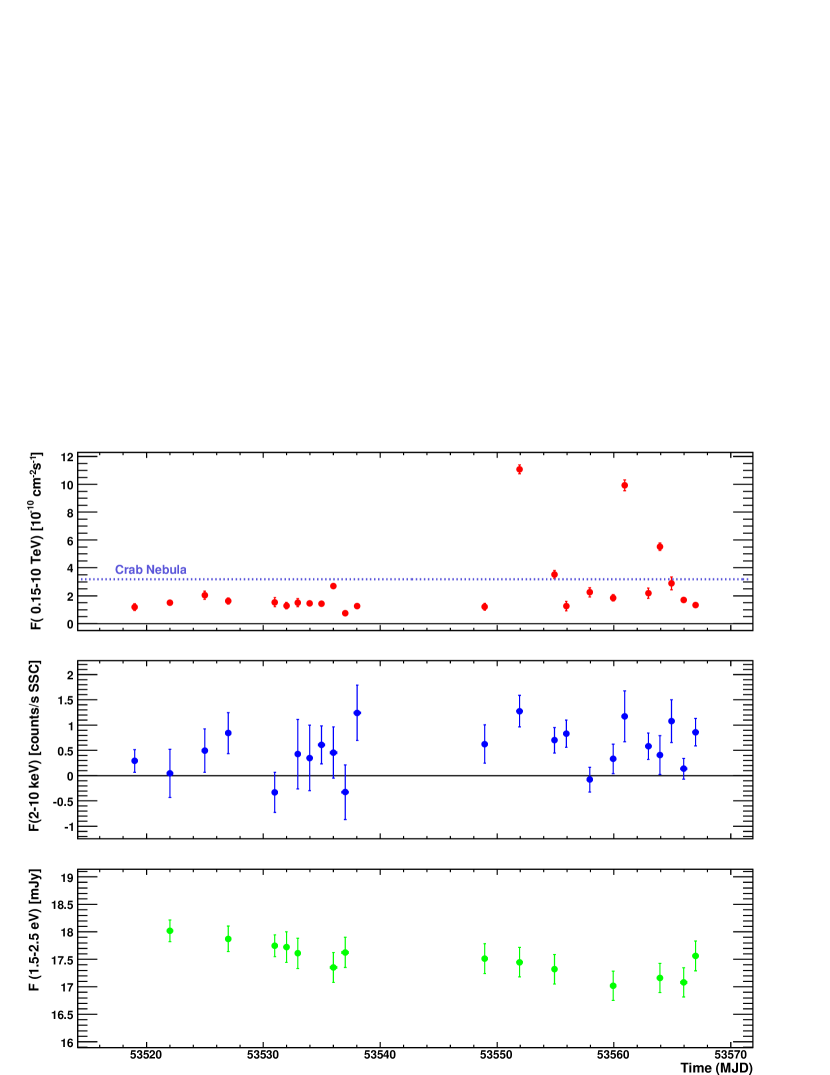
Figure 1: Multi-frequency LC during the MAGIC observations of Mrk 501 (May-July 2005). Top) MAGIC flux above 0.15 TeV. The Crab flux is also shown for comparison (lilac dotted horizontal line). Middle) $RXTE$/ASM 2-10 keV flux. Bottom) KVA $\sim$1.5-2.5 eV flux. Error bars denote 1$\sigma$ statistical uncertainties. The X-ray/optical data were selected to match the MAGIC data within a time window of 0.2 days.

The overall LC of Mrk 501 during the MAGIC observation campaign is shown in Fig. 1. The observed flux is shown in three energy bands: VHE (0.15TeV-10TeV), X-rays (2keV-10keV), and optical (1.5eV-2.5eV) as measured by MAGIC, RXTE/ASM  and KVA, respectively. The X-ray and optical fluxes are computed as weighted averages using RXTE/ASM and KVA measurements taken simultaneously with the MAGIC observations plus/minus a time tolerance of 0.2 days. A smaller time tolerance substantially decreases the number of X-ray points that can be used. The flux level of the Crab Nebula (lilac-dashed horizontal line in the top plot) is also shown in Fig. 1 for comparison. The Crab Nebula flux was obtained by applying the very same analysis as described in Sect. 2.3 to the MAGIC Crab Nebula data taken during December 2005 under observing conditions similar to those for Mrk 501. The estimated Crab Nebula flux level is therefore roughly affected by the same systematics as the fluxes obtained for Mrk 501. We found $F_{\rm Crab}$($>$$0.15\,$TeV)=(3.2$\pm$0.1)$\times$$10^{-10}$ cm^-2s^-1, thereafter referred to as Crab Unit (c.u.). For simplicity, only the Crab Nebula flux level, and not the associated error (which is irrelevant for the comparison) is shown in the LC.

The measured VHE flux from Mrk 501 was at about 0.5 c.u. during most of the observation nights (Table 1). During several nights, however, its flux significantly exceeded 0.5 c.u., and during one night (MJD 53536.947) it showed a substantially lower flux (0.24$\pm$0.04 c.u.). Often, Mrk501 showed large flux variations in consecutive nights. An example of these rapid flux variations are the MJD 53535.934 and 53536.947 with respective fluxes of 0.84$\pm$0.04 c.u. and 0.24$\pm$0.04 c.u.; the MJD 53554.906 and 53555.914 with respective fluxes of 1.11$\pm$0.09 c.u. and 0.40$\pm$0.11 c.u.; and the MJD 53563.921 and 53564.917 with respective fluxes of 1.74$\pm$0.09 c.u. and 0.91$\pm$0.15 c.u.. Besides, the VHE flux from Mrk 501 was outstanding during the MJD 53551.905 (June 30) and 53560.906 (July 09) with 3.48$\pm$0.10 c.u. and 3.12$\pm$0.12 c.u., respectively. During these two nights the source was in a very active state. Note, however, that the night before the July 9 flare the emitted flux was 0.58$\pm$0.07 c.u., i.e. close to the average flux of the entire campaign. Mrk 501 therefore showed a remarkably fast VHE variability during this campaign.

Unlike in VHE $\gamma$-rays, no significant flux variation was recorded in the X-ray and optical bands. In the case of the X-ray data, however, although the sensitivity of the RXTE/ASMinstrument was clearly inadequate to reveal short-term 2-10 keV flux variability in Mrk 501’s emission, the flux appears to be higher in the second portion of the LC. The optical flux, on the other hand, shows only a modest variation, a $\sim$$5\%$ monotonic decrease during the entire observational campaign.

3.2 Multi-frequency correlations

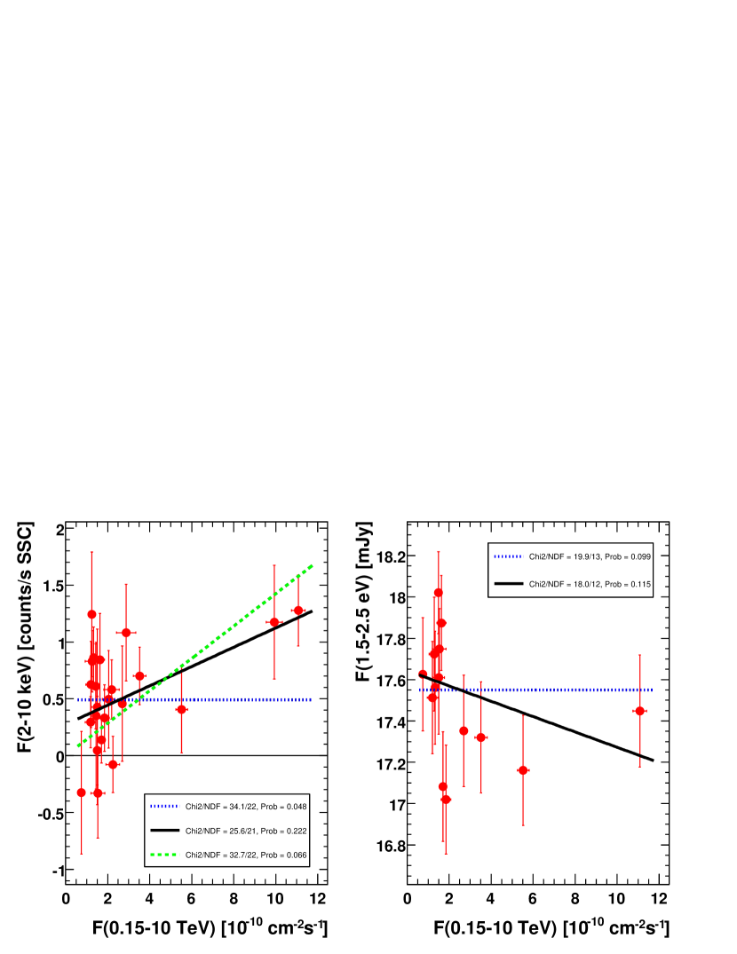
Figure 2: VHE versus X-ray (left) and optical (right) flux correlation during the MAGIC observation campaign. The data points are the same as in Fig. 1. The blue dotted lines denote constant fits; black solid and green dashed lines correspond to linear fits with/without offset (see insets for goodness-of-fits values).

The correlations of our observed VHE $\gamma$-ray data with X-ray and optical data are shown in Fig. 2, the gamma points being the same as shown in the light curve of Fig. 1. It can be seen that the measurement uncertainties of the X-ray and optical fluxes are comparatively large, which makes possible different dependencies of the X-ray flux on the $\gamma$-ray flux. We fit the VHE/X-ray data with a constant and with a linear function, obtaining the highest probability for the linear function. For the relation VHE/optical data, the two fits are nearly equally probable. All fit results are shown in the insets of Fig. 2, including for the VHE/X-ray data also a fit forcing the linear function through the origin.

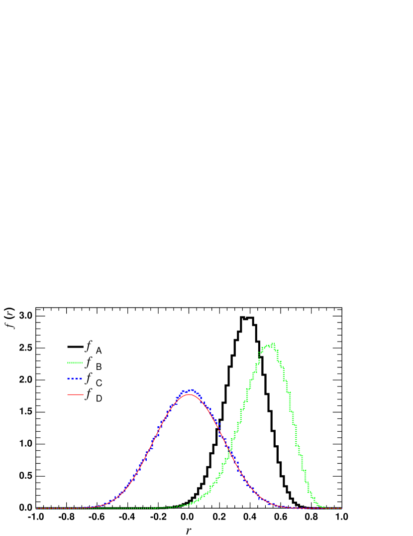
Figure 3: Probability density functions of the correlation coefficient between $\gamma$-ray and X-ray fluxes: $f_{A}$ data, $f_{B}$ perfectly correlated case, $f_{C}$ uncorrelated case, and $f_{D}$ analytical solution in the uncorrelated case. See text for further details.

For the VHE/X-ray correlation, one obtains a linear correlation coefficient of 0.49. Investigating the uncertainty of this result, we used a procedure of Monte Carlo-generated correlations, as described in detail by Ferenc & Hrupec (2007); Hrupec (2007). For all points (corresponding VHE and X-ray fluxes), multiple (we used 100 000) possible sets of measurements are generated, using random differences derived from the (Gaussian) errors assigned to each point. For each set of generated points, a correlation coefficient is obtained, resulting for a large number of measurements in the probability density function (pdf) of correlation coefficients $f_{A}(r)$ shown in Fig. 3, which corresponds to the measured correlation and the assigned errors. This pdf correctly expresses the effect of the measurement uncertainties. The same procedure can be applied to hypothetical fully correlated data: to this end, the data points are shifted onto the straight line from the fit with the highest probability (black line in left-hand plot of Fig. 3), maintaining the original error assignments. In the case of hypothetical uncorrelated data, the points are randomly distributed in the VHE/X-ray plane. Sets of Monte Carlo measurements are then generated as before. The resulting pdfs express the probability to obtain certain values of correlation coefficients, given respectively no correlation ($f_{C}(r)$ in Fig. 3) or full correlation ($f_{B}(r)$ in Fig. 3) with our error assumptions. For comparison purposes, Fig. 3 also shows the analytical pdf function for the uncorrelated case, $f_{D}(r)$ (described in chapter 9 and appendix C of (Taylor, 1997)), which does not take into account measurement errors. Note that $f_{C}(r)$ is very similar to $f_{D}(r)$. This is not surprising, since the smearing does not increase the randomness of the already randomized seed event. The width of the probability density distribution $f_{D}(r)$ depends exclusively on the number of points in the data sample (23 in our case). On the other hand, $f_{B}(r)$ is significantly affected by the measurement errors; even under the hypothesis of a fully correlated case, the probability to obtain values for the correlation coefficient larger than 0.8 is very small.

A measure of the probability of correlation can be derived from the comparison of the probability density distribution $f_{A}(r)$ for the actual measurement with the distributions for the two extreme correlation cases, $f_{B}(r)$ and $f_{C}(r)$. Given the results in Fig. 3, it is evident that $f_{A}(r)$ is similar to $f_{B}(r)$, but, despite a sizable overlap, rather different from $f_{C}(r)$. For a quantitative comparison, we followed the robust method from Poe et al (2005), which is based on the convolution of empirical probability density distributions. The comparison of a pair of probability density functions $f_{X}(r)$ and $f_{Y}(r)$ leads to the probability that these two distributions are statistically consistent, $P(f_{X}(r),f_{Y}(r))$. The resulting value for the probability of agreement between our data points and the fully correlated case, $P_{X,\gamma}(f_{A},f_{B})$, is $0.55\pm 0.15$, being the quoted error a systematical error estimated through variations in the initial values used in the Monte Carlo method (Ferenc & Hrupec, 2007; Hrupec, 2007). The probability that our measurement came as a result of a statistical fluctuation of an entirely uncorrelated physics case, on the other hand, is significantly lower; $P_{X,\gamma}(f_{A},f_{C})$ is $0.15\pm 0.05$. The probability for the first scenario to be true and for the second to be false is $P_{X,\gamma}(f_{A},f_{B})(1-P_{X,\gamma}(f_{A},f_{C}))=0.47$, and the probability for the opposite is $(1-P_{X,\gamma}(f_{A},f_{B}))P_{X,\gamma}(f_{A},f_{C})=0.067$, which indicates that the correlation scenario is significantly more likely.

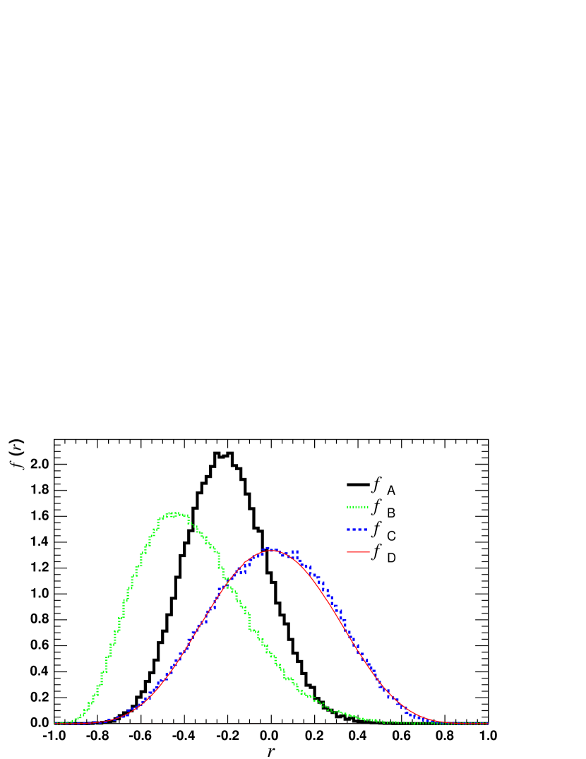
Figure 4: Probability density functions of the correlation coefficient between $\gamma$-ray and optical fluxes: $f_{A}$ data, $f_{B}$ perfectly correlated case, $f_{C}$ uncorrelated case, and $f_{D}$ analytical solution in the uncorrelated case. See text for further details.

The same method was applied to the optical and $\gamma$-ray flux values of Fig. 2 (right-hand plot). The corresponding probability density functions are presented in Fig. 4. In this case, the resulting linear correlation coefficient is -0.27, indicating a small anti-correlation; yet the probabilities $P_{{\rm opt},\gamma}(f_{A},f_{B})$$=$0.60$\pm$0.25, and $P_{{\rm opt},\gamma}(f_{A},f_{C})$=0.55$\pm$0.25 are practically equal, which suggest that neither the anti-correlated, nor the uncorrelated scenario may be reliably excluded. The probability for the first scenario to be true and for the second to be false is 0.27, while the probability for the opposite case is 0.22, which confirms the previous conclusion.

3.3 Intra-day $\gamma$-ray flux variations

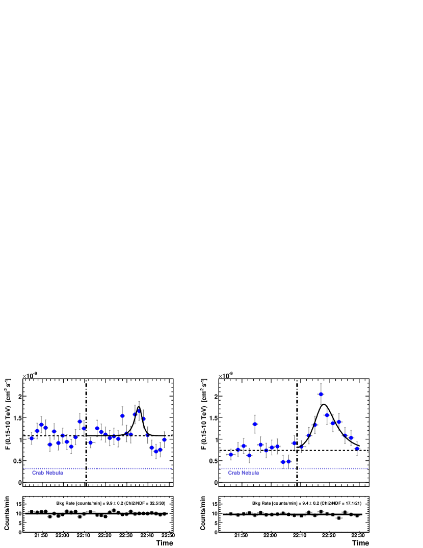
Figure 5: Integrated-flux LCs of Mrk 501 for the flare nights of June 30 and July 9. Horizontal bars represent the 2-minute time bins, and vertical bars denote 1$\sigma$ statistical uncertainties. For comparison, the Crab emission is also shown as a lilac dotted horizontal line. The vertical dot-dashed line divides the data into ’stable’ (i.e., pre-burst) and ’variable’ (i.e., in-burst) emission. The horizontal black dashed line represents the average of the ’stable’ emission. The solid black curve represents the best-fit flare model (see eq. 2). The bottom plots show the mean background rate during each of the 2-minute bins of the LCs. The insets report the mean background rate during the entire night, resulting from a constant fit to the data points. The goodness of such fit is also given.

During the two nights with the highest VHE activity, namely June 30 and July 9, Mrk 501 clearly showed intra-night flux variations. The corresponding LC in the 0.15-10 TeV band is shown in Fig. 5 with a time binning of $\sim$2 minutes. For comparison, the Crab Nebula flux is shown as a lilac dashed horizontal line. The vertical dot-dashed line divides the data into a region of relatively ’stable’ (pre-burst) emission and one of ’variable’ (in-burst) emission. The background rate after the gamma/hadron selection cuts was evaluated during these two nights, and is shown in the bottom panels of Fig. 5. These rates were found to be constant along the entire night. Consequently, the variations seen in the upper panels of Fig. 5 correspond to actual variations of the VHE $\gamma$-ray flux from Mrk501, thus ruling out detector instabilities or atmospheric changes.

A constant line fit to the whole LC gives a $\chi^{2}/NDF=47.9/30$ (probability $p=2.0\times 10^{-2}$) for the night of June 30, and a $\chi^{2}/NDF=80.6/21$ ($p=6.4\cdot 10^{-9}$) for the night of July 9. The emission above 0.15 TeV during the two nights is therefore statistically inconsistent with being constant and it is more reasonable to only fit the first part, i.e. the ’stable’ emission, with a constant - and not the entire LC. A constant fit to the ’stable’ portion of the LCs gives $\chi^{2}/NDF=13.4/12$ ($p$=0.34) for June 30, and $\chi^{2}/NDF=17.8/11$ ($p$=0.09) for July 9 (see Fig. 5). The probability that the ’variable’ parts of the LCs are compatible with the ’stable’ flux level is given by $\chi^{2}/NDF=34.5/18$ ($p=1.1\times 10^{-2}$) for June 30 and $\chi^{2}/NDF=83.3/10$ ($p=1.1\cdot 10^{-13}$) for July 9, respectively. We therefore measured intra-night flux variations in both nights.

The flare’s amplitude and duration, as well as its rise/fall times, can be quantified according to

$$F(t)=a+\frac{b}{2^{-\frac{t-t_{0}}{c}}+2^{\frac{t-t_{0}}{d}}}$$ (2)

(Schweizer, 2004). This model parameterizes a flux variation (flare) superposed on a stable emission: $F(t)$ asymptotically tends to $a$ when $t\rightarrow\pm\infty$. The parameter $a$ is the assumed constant flux at the time of the flare (cf. the horizontal black dashed lines in Fig. 5); $t_{0}$ is set to the time corresponding to the point with the highest value in the LC; and $b,c,d$ are left free to vary. The latter two parameters denote the flux-doubling rise and fall times, respectively, and can be converted into the characteristic rise/fall times by multiplying them by $1/ln2$. The resulting fits using eq. 2 are shown in Fig. 5, and their parameter values are reported in Table 2. In both cases, the measured rise/fall flux-doubling times are $\sim$2 minutes, which yields characteristic rise/fall times of 2/ln2 $\sim$3 minutes. These are the shortest flux-variation timescales ever measured from Mrk 501, at any wavelength.

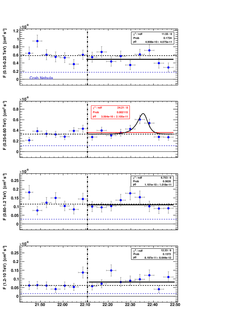
Figure 6: LC for the night June 30 with a time binning of 4 minutes, and separated in different energy bands, from the top to the bottom, 0.15-0.25 TeV, 0.25-0.6 TeV, 0.6-1.2 TeV, 1.2-10 TeV. The vertical bars denote 1$\sigma$ statistical uncertainties. For comparison, the Crab emission is also shown as a lilac dotted horizontal line. The vertical dot-dashed line divides the data into ’stable’ (i.e., pre-burst) and ’variable’ (i.e., in-burst) emission emission. The horizontal black dashed line represents the average of the ’stable’ emission. The ’variable’ (in-burst) of all energy ranges were fit with a constant line. The results of the fits are given in the insets. The constant line fit on the energy range 0.25-0.6 TeV was not satisfactory (see inset in figure); yet this LC could be fit with the flare model described by equation 2 (see table 3 for the resulting parameters).

Because of the steeply falling spectra, the low-energy events dominate the LCs shown in Fig. 5, and tend to hide any higher-energy features. We therefore split the data into four distinct energy ranges: 0.15-0.25 TeV, 0.25-0.6 TeV, 0.6-1.2 TeV and 1.2-10 TeV. The corresponding LCs for the night June 30 are shown in Fig. 6. Due to the reduced photon statistics, we increased the time binning from 2 minutes to 4 minutes. We found that only the energy range 0.25-0.6 TeV shows a clear flux variation; a constant line fit gave $\chi^{2}/NDF=24.2/8$ ($p=2\cdot 10^{-3}$). The other energy ranges are compatible with a constant line fit, showing only a slight overall flux level variation with respect to the LC in the ’stable’ part. Therefore, if there is a flux variation, it is too small to be significantly seen in our data. Note that, among the 4 energy ranges used, the 0.25-0.60 GeV energy range is the one with the highest sensitivity for flux variations. The ’variable’ LC from the energy range 0.25-0.60 TeV was then fitted using equation 2, fixing $t_{0}$ to the time of the highest point in the LC. The resulting parameters of the fit are reported in table 3; the rise/fall flux-doubling times are comparable to those ones obtained using the integrated LC above 0.15 TeV.

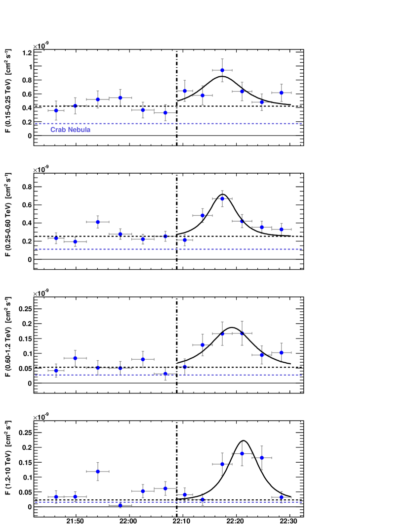
Figure 7: LC for the night July 9 with a time binning of 4 minutes, and separated in different energy bands, from the top to the bottom, 0.15-0.25 TeV, 0.25-0.6 TeV, 0.6-1.2 TeV, 1.2-10 TeV. The vertical bars denote 1$\sigma$ statistical uncertainties. For comparison, the Crab emission is also shown as a lilac dotted horizontal line. The vertical dot-dashed line divides the data into ’stable’ (i.e., pre-burst) and ’variable’ (i.e., in-burst) emission emission. The horizontal black dashed line represents the average of the ’stable’ emission. The ’variable’ (in-burst) of all energy ranges were fit with a flare model described by equation 2, where $c=d$ (rise=fall time). All parameters were left free in the fit. All light curves were considered simultaneously in the fit (combined fit). The resulting parameters from this combined fit are reported in table 4.

The same exercise on the flare July 9 gave a significantly different result, as shown in Fig. 7. The flare is visible essentially in all energy ranges. In order to study possible time shifts between the different energy ranges, we fit all LCs simultaneously (combined fit) with a flare model described by equation 2. In order to remove one degree of freedom and facilitate the fit procedure, we assume a symmetric flare with equal rise and fall flux-doubling times; that is $c=d$ in equation 2. The resulting parameters from this combined fit are shown in table 4. The combined fit gave $\chi^{2}/NDF=14.0/12$ ($p=0.3$), which implies that the measured flare is compatible with being symmetric. The rise/fall flux-doubling time is about 2 minutes for all the energy ranges. It is interesting to note that the position of the peak of the flare for the different LCs seems to vary somewhat with energy. The time difference between the highest energy range and the lowest energy range is 239 $\pm$ 78 seconds. If instead, the energy range 0.25-0.6 TeV is selected as the lowest energy range, which has a better defined flare (and thus a better determination of the peak position), the time difference is 232 $\pm$54 seconds.

In order to evaluate the significance of this time shift, we performed the same fit, but this time using a common $t_{0}$ for all LCs. The resulting fits are shown in Fig. 8, and the resulting parameters from the fit in table 5. The combined fit gave $\chi^{2}/NDF=26.6/15$ ($p=0.04$), which implies that such a situation is unlikely, and consequently that the time shift of 4 $\pm$ 1 min between the highest and the lowest energies is more probable.

Investigating the reliability of the time delay obtained from the combined fit, we performed a cross-correlation analysis on the LCs from July 9 with the methodology described in section 3.2. For this study we used LCs with 2 min time bins from the energy ranges 0.25-0.6 TeV and 1.2-10 TeV. The correlation coefficient and probability of correlation were computed after introducing time shifts of 2 min (one bin in the LCs). We obtained the highest values for a time lag of 4 minutes; which is consistent with the results from the combined fit shown above.

We want to point out that this is the first time that a possible time delay between flares at different energies is observed at VHE $\gamma$-ray energies, although such time lags have been detected for some TeV blazars at X-ray frequencies, viz. Mrk 421 (Ravasio et al, 2004) and PKS 2155-304 (Zhang et al, 2006a, b). If the observed VHE time lag is assumed real, this suggests that we are observing the underlying dynamics of the relativistic electrons in both the synchrotron and IC emission, and the observation, therefore, supports SSC models.

It should be also noted that the relative amplitude of the flux variations observed in the LC for July 9 with respect to the baseline emission, is significantly larger at the highest energies. This can be seen from the ratio $b/a$, where $a$ and $b$ are the coefficients in eq. 2 describing, respectively, the baseline and amplitude of the flare (see table 4): $b/a=3.6\pm 1.0$ and 17$\pm$4 for, respectively, the 0.25-0.6 TeV and 1.2-10 TeV bands. The July 9 LC also shows some significant flux variation in its ’stable’ part: in the highest-energy band, where activity is most conspicuous, a constant fit gives a $\chi^{2}/NDF=20.6/5$ ($p=9.6\cdot 10^{-4}$).

In summary, during the 2005 MAGIC observations of Mrk 501 we detected variability at VHE frequencies with flux-doubling times down to 2 minutes. This is about 50 times faster than the shortest previously observed variability-times at VHE frequencies for Mrk501 (Hayashida et al, 1998; Quinn et al, 1999; Aharonian et al, 1999a; Djanati-Ataïet al, 1999), and about 5 times shorter than the shortest observed variability for Mrk 421 (Gaidos, 1996). The above presented flux-variations are among the shortest ever observed in blazars, see also Aharonian et al (2007). It is interesting to note that the Mrk 501 flux-doubling rise times observed by MAGIC in the VHE range are rather comparable to the shortest variability times observed at X-ray frequencies which were reported by Xue & Cui (2005): a flare with a total duration of 15 minutes with a flux variation of 30%. The authors, however, reported the presence of substructures, which point to the existence of variability on timescales shorter than 15 minutes. It is worth mentioning that for both X-ray and $\gamma$-ray  the shortest flux varitions occurred when the source was not in an exceptionally high emission state.

3.4 Quantification of the variability

Mrk 501 has shown energy-dependent flux variations throughout the entire MAGIC observational campaign. We followed the description given in Vaughan et al (2003) to quantify the flux variability by means of the fractional variability parameter $F_{var}$, as a function of energy. In order to account for the individual flux measurement errors ($\sigma_{err,i}$), we used the ’excess variance’ (Nandra et al, 1997; Edelson et al, 2002) as an estimator of the intrinsic source variance. This is the variance after subtracting the expected contribution from measurement errors. For a given energy range, the $F_{var}$ is calculated as

$$\mbox{$F_{var}$}=\sqrt{\frac{S^{2}-<\sigma_{err}^{2}>}{<F_{\gamma}>^{2}}}$$ (3)

where $<F_{\gamma}>$ is the mean photon flux, $S$ the standard deviation of the $N$ flux points, and $<\sigma_{err}^{2}>$ the average mean square error, all determined for a given energy bin. The uncertainty on $F_{var}$ is estimated according to:

$$\Delta\mbox{$F_{var}$}=\sqrt{\Big{(}\sqrt{\frac{1}{2N}}\cdot\frac{<\sigma_{err}^{2}>}{<F_{\gamma}>^{2}\cdot\mbox{$F_{var}$}}\Big{)}^{2}+\Big{(}\sqrt{\frac{<\sigma_{err}^{2}>}{N}}\frac{1}{<F_{\gamma}>}\Big{)}^{2}}$$ (4)

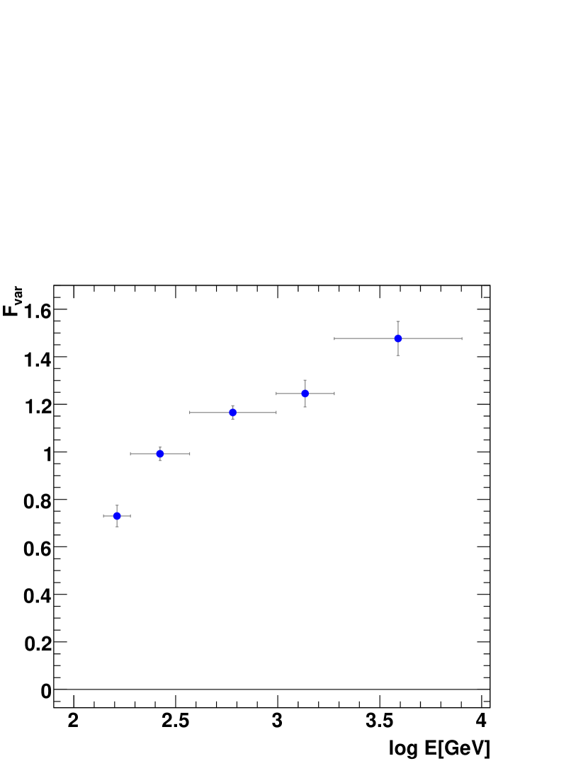
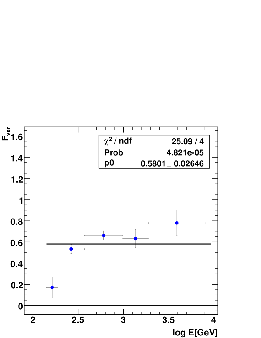
Figure 9: Fractional variability parameter as derived for 5 energy bins. Vertical bars denote 1$\sigma$ uncertainties, horizontal bars indicate the width of each energy bin. The left plot includes all data. The right plot includes all but the June 30 and July 9 data. The black horizontal line in the right panel results from a constant fit to the data points (see inset for fit parameters).

Fig. 9 shows the derived $F_{var}$ values for 5 logarithmic energy bins, spanning from 0.14 TeV to 8 TeV. The left-hand plot includes all data, while the right-hand plot includes all data except for the two active nights. The result indicates a larger-amplitude flux variation at higher energies, which is clearly discernible even when the active-state data are excluded (the null probability being $p$$\sim$$10^{-5}$).

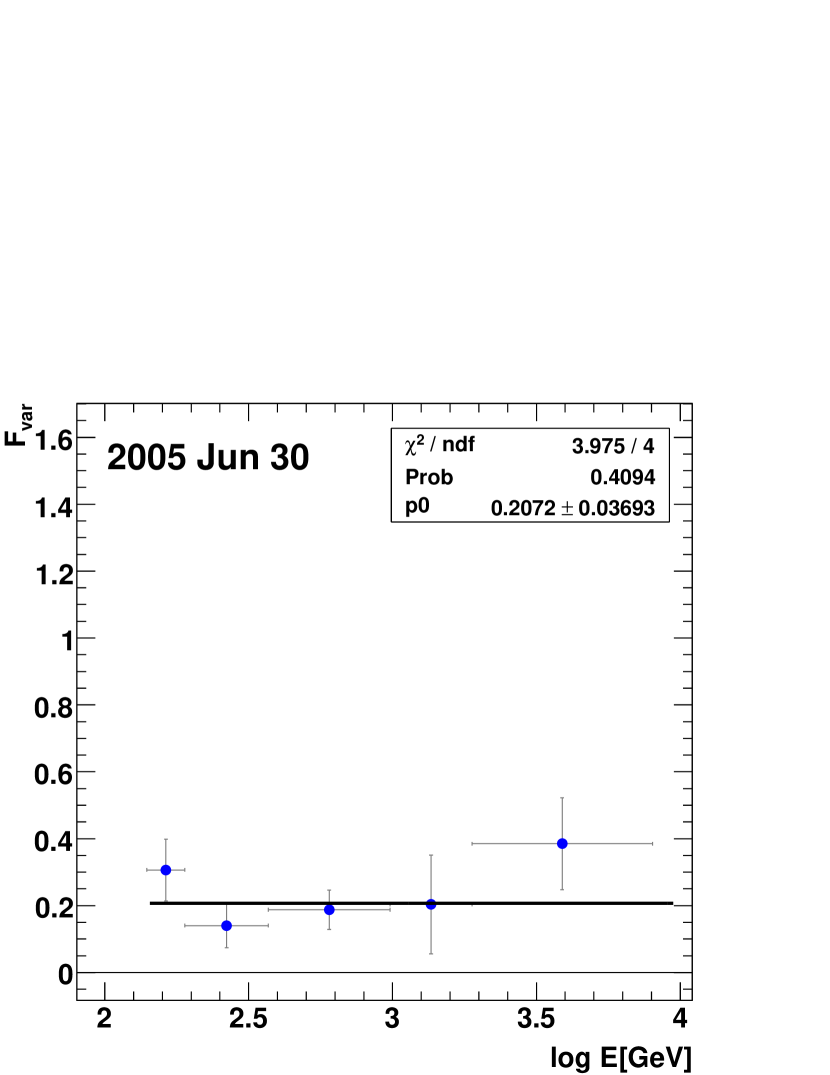
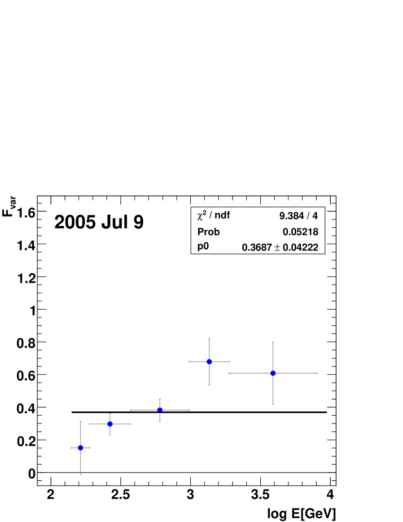
Figure 10: Fractional variability parameter as computed for the nights of June 30 and July 9. Vertical bars denote 1$\sigma$ uncertainties, horizontal bars indicate the width of each energy bin. The black horizontal lines are the result of a constant fit to the data points (see inset for fit parameters).

Fig. 10 shows the $F_{var}$ values as derived for the individual active nights of June 30 and July 9. The flux variability in these nights is smaller than for the entire observational campaign, as one would expect from simple inspection of Fig. 1. In the night of June 30, $F_{var}$ does not increase significantly with energy. In contrast to June 30, there is a clear increase of $F_{var}$ with energy in the night of July 9 - in spite of the larger error bars coming from a shorter observation time and a lower mean flux.

In summary, during the year 2005 MAGIC observations, the VHE $\gamma$-ray flux variability of Mrk 501 was found to significantly increase with energy, on time scales from months to less than an hour. A similar effect (on timescales $\sim$$>$ 1/2 hr) was also detected in X-rays in 1997, 1998, and 2000 (Gliozzi et al (2006), based on RXTE data). Another X-ray evidence was found for the TeV blazar: PKS 2155-304 (Zhang et al, 2006b). The largest X-ray $F_{var}$ value in X-rays for Mrk 501 was $\sim$0.6-0.7 in the highest energy bin at 10-20 keV, and it was found in June 1998 and July-September 2000 (Gliozzi et al (2006)). In 1997 however, despite Mrk 501 showed the highest X-ray (2-10 keV) fluxes from the last ten years, the largest observed $F_{var}$ value in X-rays  was only $\sim$0.4. It is interesting to note that, in the VHE $\gamma$-ray range, we observe a maximum $F_{var}$ of $\sim$$>$ 0.6, which increases to $\sim$$>$ 1.2 when the two active nights are included. This suggests that Mrk 501 is more variable in VHE $\gamma$-rays than in X-rays.

4 VHE Spectra

The differential photon spectra of Mrk 501 were parameterized with a simple power-law (PL) function:

$${dF\over dE}=K_{0}\cdot\Big{(}\frac{E}{0.3\mbox{TeV}}\Big{)}^{-a}$$ (5)

where $K_{0}$ is a normalization factor and $a$ the photon index. The MAGIC sensitivity permits to derive VHE spectra of Mrk 501 on a daily basis, independent of its flux level, a real asset for unbiased precision studies of blazars. The PL spectral parameters for each single night are reported in Table 1.

During our observations the VHE emission of Mrk 501 showed a very dynamic behaviour, with significant spectral variability on a timescale of days (see Sect. 4.1 and 4.2). Nevertheless, most of the data are well described by the simple PL function of eq. 6. This does not hold for the two flaring nights of June 30 and July 9 which are therefore discussed separately in Sect. 4.3 and 4.4.

4.1 Spectral index vs. flux

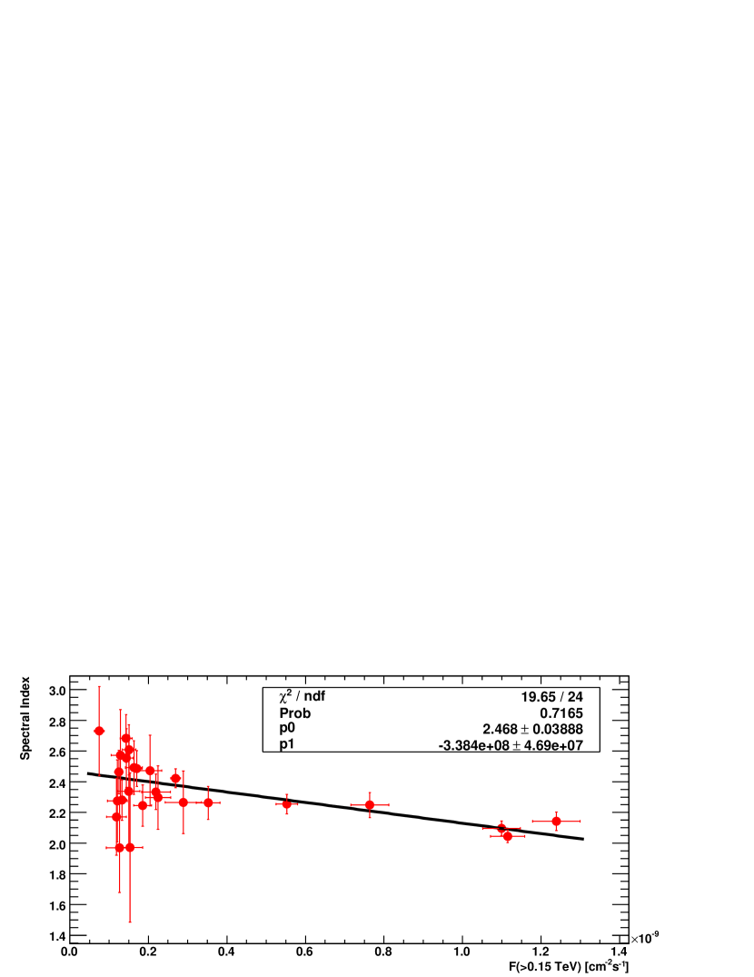
Figure 11: Correlation between spectral shape and integrated flux above 0.15 TeV. Each point denotes a single night of observation. The error bars denote 1$\sigma$ uncertainties. The June 30 and July 9 data were split chronologically into two data sets each, corresponding to the pre-flare (’stable’) and in-flare (’variable’) emission shown in figure 5.

The Mrk 501 VHE spectrum was measured on a night-by-night basis, which allowed investigating possible correlations between the PL spectral index and intensity, as it is shown in Fig. 11. The data of June 30 and July 9 were again split into the ’stable’ and ’variable’ part (see Fig. 5) and consequently, Fig. 11 contains 26 instead of 24 points. The data points are well described by a linear fit; but a constant is clearly excluded ($\chi^{2}/NDF=74.7/25$, i.e. $p=7.4\cdot 10^{-7}$). On average, the Mrk 501 spectrum hardens when the emission increases. Such a correlation was already reported by Pian et al (1998); Tavecchio et al (2001), although on substantially longer timescales.

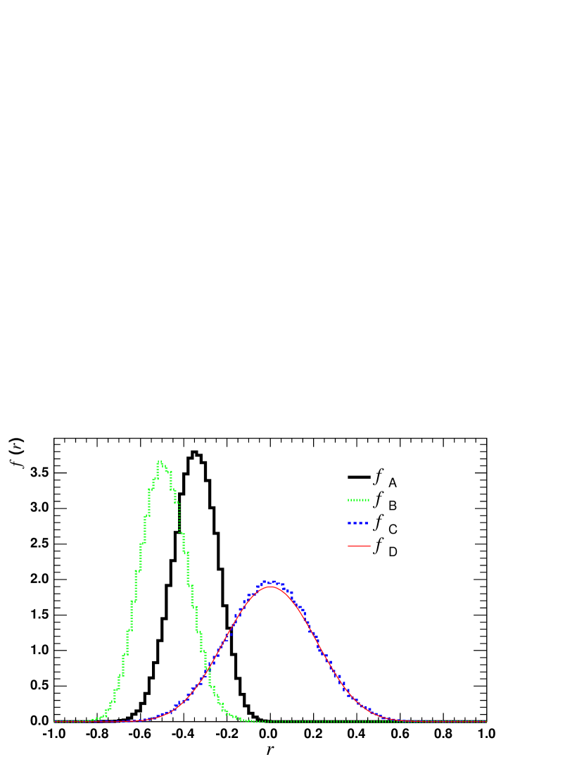
Figure 12: Probability density functions of the correlation coefficient between spectral index and $\gamma$-ray fluxes: $f_{A}$ data, $f_{B}$ perfectly correlated case, $f_{C}$ uncorrelated case, and $f_{D}$ analytical solution in the uncorrelated case. See text for further details.

In order to test the ansatz of a linear correlation in spectral index versus $\gamma$-ray flux (see Fig. 11), we applied a correlation analysis as described in Sect. 3.2. The linear fit indicates anti-correlation ($\chi^{2}/{\rm ndf}=19.65/24$, $p$$=$$0.72$). The correlation factor is -0.48, and the corresponding probability distributions are shown in Fig. 12. We find the probability $P_{\alpha,\gamma}(f_{A},f_{B})=0.35$, to be higher than $P_{\alpha,\gamma}(f_{A},f_{C})=0.12$, which supports a modest anti-correlation.

Similar, the probability for the first scenario to be true and for the second to be false is $P_{{\alpha},\gamma}(f_{A},f_{B})(1-P_{{\alpha},\gamma}(f_{A},f_{C}))=0.30$, while the probability for the opposite case is $(1-P_{{\alpha},\gamma}(f_{A},f_{B}))P_{{\alpha},\gamma}(f_{A},f_{C})=0.08$. In conclusion, this correlation study indicates a spectral hardening with increased flux.

4.2 Spectra at different flux levels

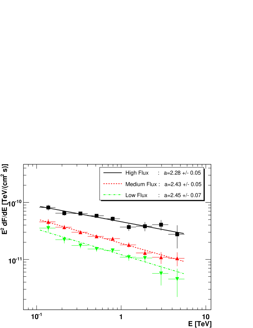
Figure 13: Measured spectra of Mrk 501 for three different $>$0.15 TeV flux levels: low (green down triangles), medium (red up triangles), and high (black squares). Vertical bars denote 1$\sigma$ uncertainties, horizontal bars denote energy bins. Lines show power-law best fits. See table 6 for fit parameters.

In order to investigate the spectra at different flux levels, the diurnal data were combined into three groups, depending on whether the integral flux above 0.15 TeV, $F_{0.15\,{\rm TeV}}$ (measured in Crab Units (c.u.)), was low ($F_{0.15\,{\rm TeV}}$$<$$0.5~{}\mbox{c.u.}$), medium ($0.5~{}\mbox{c.u.}$$<$$F_{0.15\,{\rm TeV}}$$<1.0~{}\mbox{c.u.}$), or high ($1.0~{}\mbox{c.u.}$$<$$F_{0.15\,{\rm TeV}}$). Based on the chosen flux limits the low-, medium- and high-flux data sets consist of 12, 8 and 2 nights, respectively (see table 1 for detailed statistics). The data from June 30 and July 9 will be discussed in Sect. 4.3 and are not included in the analysis here. The differential photon spectrum for all three flux regions together with the PL fit results are shown in Fig. 13; the fit parameters are also listed in table 6. Even with such a simple parameterization, our data do suggest a spectral hardening with increasing flux. The results of this analysis are consistent with the trend seen in Fig. 11 and discussed in sect. 4.1.

The HEGRA CT system measured the spectra of Mrk 501 in 1998-1999, at a time when its flux level was substantially below the one of the Crab ($\sim$1/3 c.u.). The observation covered 122 hours (Aharonian et al, 2001). The reported spectrum could be fitted with a PL in the energy range 0.5-10 TeV, giving a spectral index of 2.76 $\pm$ 0.08. It is interesting to note that this spectral index is slightly softer than the 2.45 $\pm$ 0.07 we obtained for the low flux (17 hours of observation, $\sim$0.4 c.u.) in the energy range 0.1-6 TeV. This spectral shape difference might be caused by a possible softening of the spectra above 1-2 TeV. Note that the fits to the spectra measured by MAGIC are mostly constrained by the points below 2 TeV (due to low photon statistics at the highest energies), while the fits to the spectra measured by HEGRA are mostly constrained by the points above 1 TeV. Certainly, a factor contributing to the softening of the spectra at the highest energies is the $\gamma$-ray extinction due to pair production by interaction with the Extragalactic Background Light (EBL). According to Kneiske et al (2004), the attenuation of $\gamma$-rays coming from Mrk 501 is $\sim$30% at 1 TeV and $\sim$50% at 10 TeV, while it is $\leq$15% for energies below 0.5 TeV.

4.3 Spectra during active nights

The differential photon spectra from June 30 and July 9 were fitted with the simple PL described in eq. 5 as well as with the log-parabolic function:

$${dF\over dE}~{}=~{}K_{0}\cdot\Big{(}\frac{E}{0.3\,TeV}\Big{)}^{-a-b\cdot log_{10}\big{(}\frac{E}{0.3\,TeV}\big{)}}\,.$$ (6)

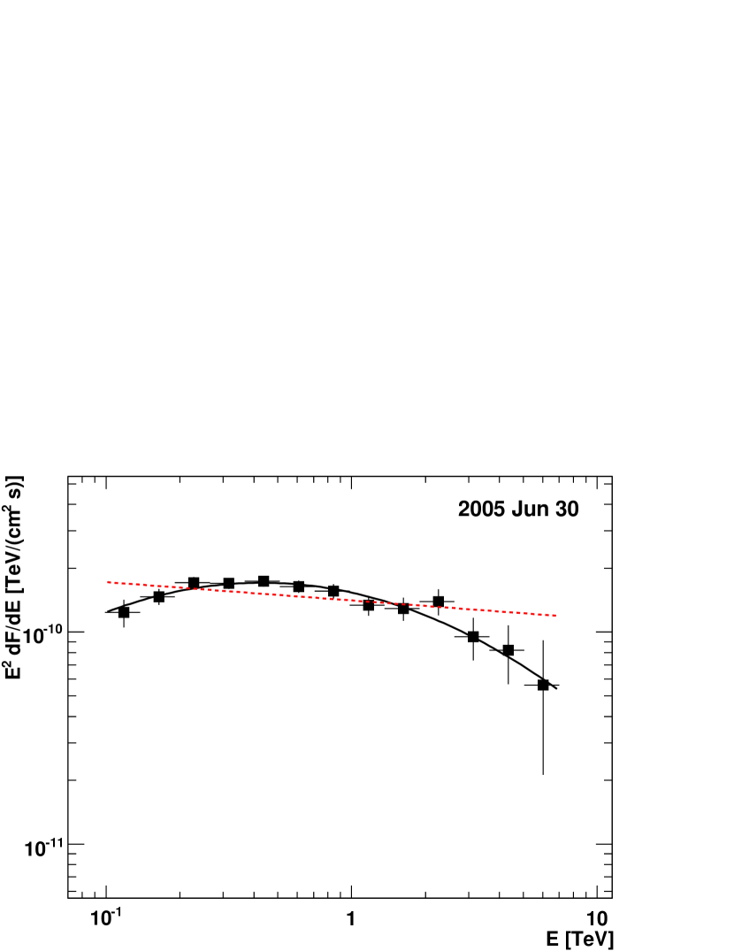
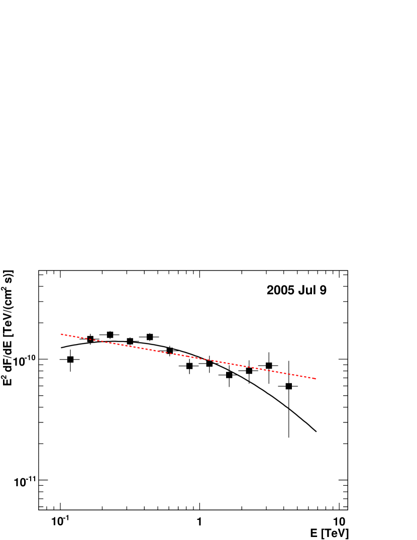
Figure 14: Measured spectra for the nights of June 30 and July 9 when Mrk 501 flared. Bars as in Fig. 13. Spectral fits are a power-law (red dashed line; see eq. 5) and a log-parabolic function (black solid line; see eq. 6). See table 7 for fit parameters.

Here, $K_{0}$ is a normalization factor, $a$ is the spectral index at 0.3 TeV, and $b$ is a curvature parameter (for $b$$>$0 the spectrum hardens/softens at energies below/above 0.3 TeV). The log-parabola is a simple function to describe curved spectra and, as pointed out by Massaro et al (2004, 2006), can be directly related to the intrinsic physical processes occurring in the source. The results of both, the power law and the log-parabolic functions are reported in Table 7. Since the log-parabolic fit describes the data more accurately than the PL fit, this suggests that the differential photon spectra of the two flaring nights are curved. The spectra and their fits are shown in Fig. 14. Note that the peak of the energy spectrum is located in the covered energy range in both nights.

The peak location in a spectrum described by eq. 6 is given by:

$$E_{peak}~{}=~{}10^{\frac{2-a}{2b}}\cdot 0.3~{}\mbox{TeV}$$ (7)

with an associated uncertainty of

$$\Delta E_{peak}~{}=~{}E_{peak}\cdot\frac{ln10}{2b}\cdot\sqrt{V_{aa}+V_{bb}\cdot\Big{(}\frac{a-2}{b}\Big{)}^{2}-2V_{ab}\cdot\Big{(}\frac{a-2}{b}\Big{)}}$$ (8)

where $V_{aa},V_{bb}$ and $V_{ab}$ are the coefficients of the covariance matrix. Using these equations one finds that the peak locations are 0.43$\pm$0.06 TeV and 0.25$\pm$0.07 TeV for the spectra measured during June 30 and July 9, respectively. It should be noted that these spectra are not corrected for EBL absorption, and are therefore not intrinsic to Mrk 501. After correction for EBL absorption the spectral peaks are shifted towards higher energies (see Sect. 5.5).

The detection of a spectral curvature and measurement of the peak location was first reported by the Whipple and CAT collaborations (Samuelson et al, 1998; Djanati-Ataïet al, 1999; Piron, 2000, 2001) based on 1997 Mrk 501 data. However, in those studies the spectra were not corrected for the EBL absorption. Such correction is relevant because the measured curvature in those energy spectra occurred essentially above 1-2 TeV, where current EBL models predict a $\geq$40% attenuation. Below 1 TeV, little (if at all) curvature could be seen within the quoted 1$\sigma$ statistical errors. Therefore, we suggest that the curvature and peak location reported in those studies may be significantly affected (if not dominated) by the EBL absorption. On the other hand, the spectral curvature in the MAGIC data is dominated by points below 1 TeV, since the higher-energy points hardly constrain the fit due to their substantially larger error bars. The curvature we measure thus is affected, but not dominated by EBL absorption.

4.4 Intra-night spectral variations

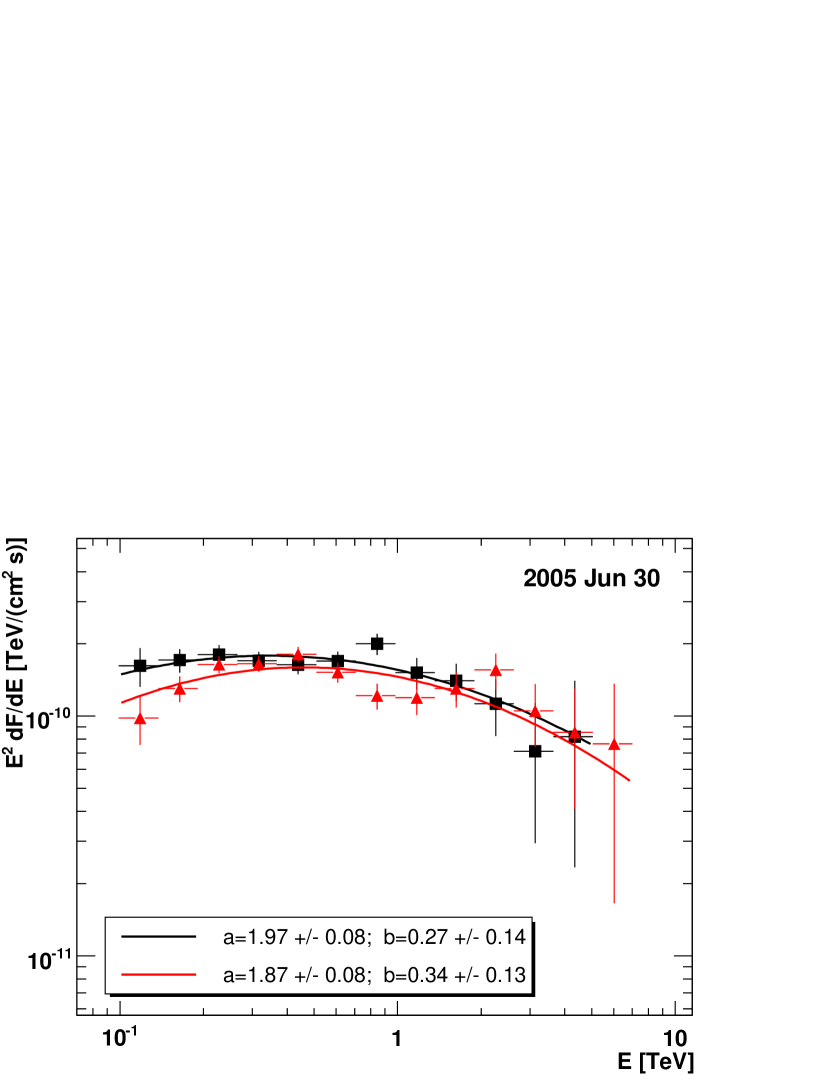
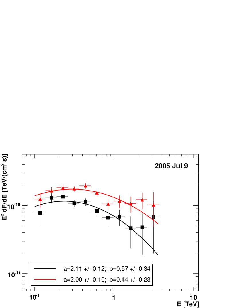
Figure 15: The spectra of Mrk 501 in the nights of June 30 and July 9 corresponding to the pre-burst (’stable’) and in-burst (’variable’) emission (see sect. 3.3 and Fig. 5). Black squares/red triangles denote ’stable’/’variable’ emission. Bars as in Fig. 13. The insets show the log-parabolic fit parameters (see eq. 6).

As discussed in section 3.3, during the active nights of June 30 and July 9 the VHE emission of Mrk 501 can be divided into a ’stable’ (pre-burst) and ’variable’ (in-burst) part. In order to study potential changes in the spectral shape, we derived the differential photon spectrum for the two parts of each night (Fig. 5). Since each spectrum is based on $\leq$1/2 hr exposure this procedure certainly increases the statistical errors. The four spectra were fitted with the log-parabolic function in eq. 6, which is preferred over the simple PL function (see sect. 4.3). The results of the fit, as well as other relevant information (e.g., net observing time, significance of the signal, goodness of fit) are reported in Table 8. The spectra and the corresponding fits are plotted in Fig. 15. In both nights, there is marginal ($~{}1\sigma$) evidence for a spectral hardening during the flare.

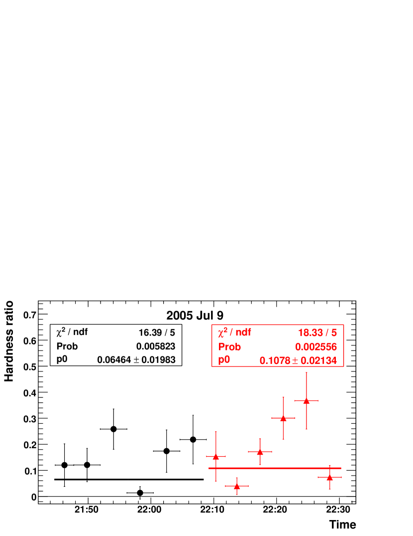
Figure 16: Hardness ratio $F(1.2-10~{}\mbox{TeV})/F(0.25-1.2~{}\mbox{TeV})$ vs $Time$ for the nights of June 30 and July 9. Horizontal bars represent the 4-minute time bins, and vertical bars denote 1$\sigma$ statistical uncertainties. Black squares and red triangles denote pre-burst (’stable’) and in-burst (’variable’) emission respectively (see sect. 3.3 and Fig. 5). The lines result from a constant fit to the data points (see insets for fit parameters).

We also studied the time-evolution of the hardness ratio, defined as the ratio
F(1.2-10 TeV)/F(0.25-1.2 TeV) and which is computed directly from the LCs shown in Fig. 6 and Fig. 7. The resulting graph is shown in Fig. 16. The hardness ratios for the pre-burst and in-burst part are quantified by means of a constant fit. In both nights the hardness ratio is somewhat larger (1-2$\sigma$) in the in-burst than in the pre-burst part, in agreement with the observed spectral hardening (see Fig. 15). It is worth noting that the hardness ratios for the pre-burst and in-burst time windows of June 30 are statistically compatible with being constant, those of July 9 are much less so, as shown in the insets of Fig. 16.

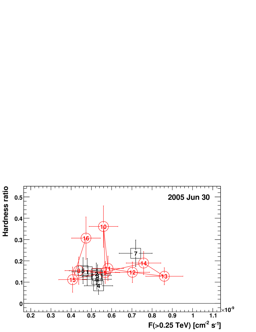
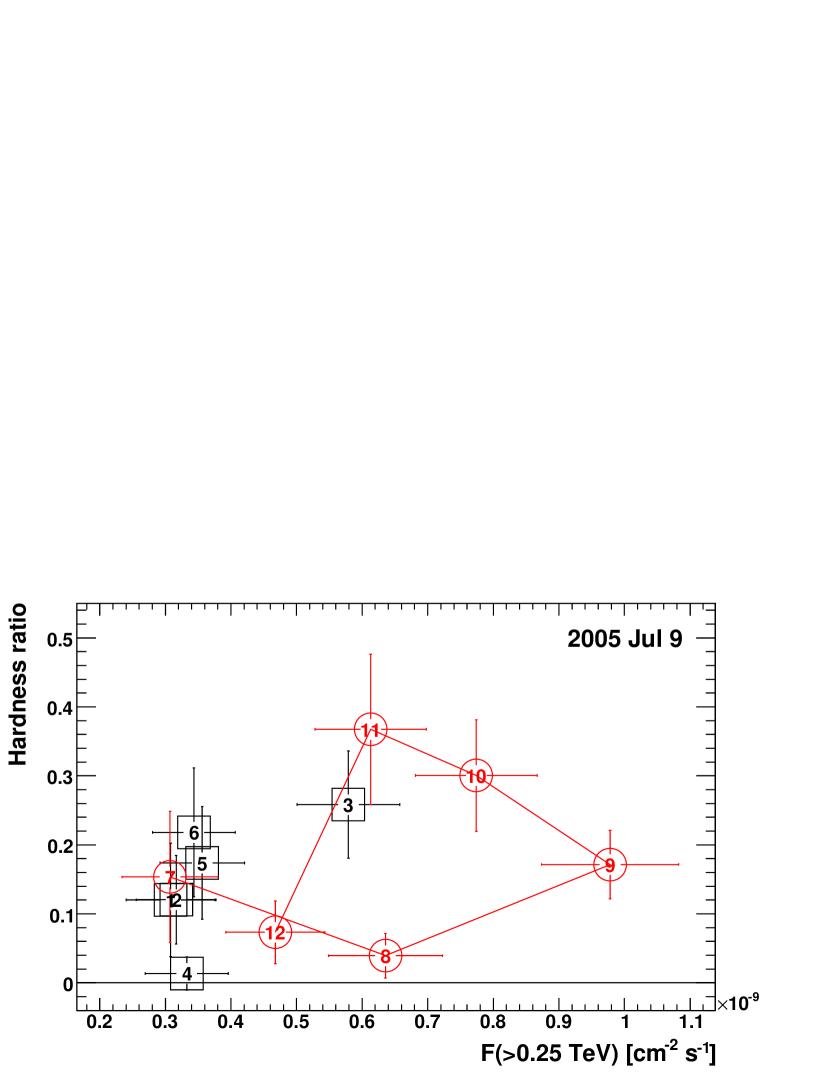
Figure 17: Hardness ratio $F(1.2-10~{}\mbox{TeV})/F(0.25-1.2~{}\mbox{TeV})$ vs $F(>0.25~{}\mbox{TeV})$ for the nights of June 30 and July 9. Horizontal and vertical bars denote 1$\sigma$ statistical uncertainties. Black open squares and red open circles denote pre-burst (’stable’) and in-burst (’variable’) emission respectively (see sect. 3.3 and Fig. 5). The numbers inside the markers denote the position of the points in the LCs. The consecutive (in time) points of the in-burst LC are connected by red lines for better clarity.

The evolution of the hardness ratio with the emitted flux above 0.25 TeV is shown in Fig. 17. Both nights show some evidence for a larger spread in the in-burst part than in the pre-burst part. The evolution of the in-burst points from June 30, however, is somewhat chaotic, while the evolution of the in-burst points from July 9 shows a clear loop pattern rotating counterclockwise. The physical interpretation of this feature is given in section 5.3. Concluding, a spectral hardening with increased emission characterizes the VHE emission of Mrk 501 also at short timescales.

5 Discussion

In this section we discuss the VHE light curve of Mrk 501 for May - July 2005 in comparison to previous IACT observations made from the years 1997 through 2000. We also discuss the observed rapid flux variability in the framework of a basic model of gradual electron acceleration. The broadband spectral features of Mrk 501 and the intrinsic VHE spectra from different activity states are discussed in the framework of a basic SSC model. We also model the ensuing intrinsic VHE spectra – corresponding to different activity states – in an SSC framework.

5.1 Historical light curve

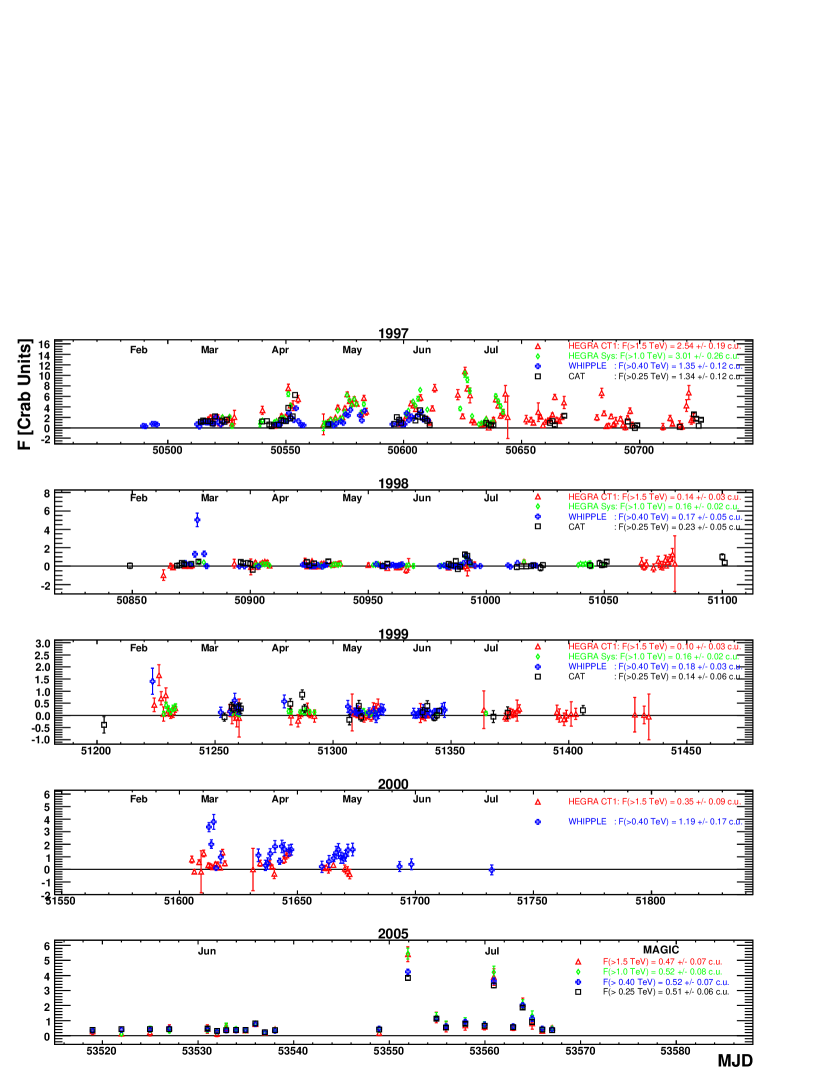
Figure 18: Single-night VHE LCs of Mrk 501 obtained with various IACTs during several years. Vertical error bars denote 1$\sigma$ statistical uncertainties. Instruments and corresponding mean fluxes are reported for each observational campaign separately. The MAGIC data were reprocessed to match the energy ranges covered by previous instruments.

It is interesting to examine Mrk 501’s VHE activity in 2005, as measured by MAGIC  in perspective to that recorded in 1997-2000 by other IACTs such as HEGRA CT1 (Kranich, 2000), HEGRA CT System (Multi-Messenger-Group, 2006), Whipple (Quinn et al, 1999), and CAT (Djanati-Ataïet al, 1999; Piron, 2001). The long-term Mrk 501 lightcurve covering the years 1997 to 2005 is shown in Fig. 18. For easier comparison among instruments covering different energy ranges, the integral flux values are given in Crab Units (c.u.). The mean fluxes for each year and instrument are shown in the insets of Fig. 18. They were derived using the exposure times as statistical weights (whenever this information was available), and excluding data points $>$ 3$\sigma$ away from each mean value, to permit a better comparison. For MAGIC, mean fluxes were computed in the other IACTs’ energy bands. In 1997, when Mrk 501 was much brighter than the Crab, Whipple and CAT fluxes were in mutual agreement, but they significantly differed from the HEGRA CT System and HEGRA CT1 fluxes; the reasons being (i) the highest-flux nights (May–July 1997) happened to be covered by HEGRA CT and CT1 but not by Whipple and CAT; and (ii) the highest threshold energies of HEGRA CT and CT1, together with the fact that when Mrk 501 is active its spectrum becomes significantly harder than the Crab’s (see Sects. 4.1 and 4.2), hence fluxes measured in Crab units are larger at higher energies. In 1998 and 1999 the various IACT data agreed on a flux of $\sim$0.15-0.20 c.u., i.e. an order of magnitude lower than in 1997. In 2000, March through May, the mean VHE flux of Mrk 501 increased to a level of 0.35$\pm$0.09 (HEGRA CT1) and 1.19$\pm$0.17 (Whipple), the main reason for the discrepancy being that HEGRA CT1 missed the nights with highest flux measured by Whipple. In 2005, May through July, the mean baseline VHE flux from Mrk 501 was $\sim$0.5 c.u., significantly lower than in 1997 and 2000, but higher than in 1998 and 1999.

A 23-day flux periodicity was claimed by Kranich (2000) using data from HEGRA CT1. Recently, Osone (2006) confirmed the 23-day periodicity at VHE frequencies and extended it to X-rays (based on ASM/RXTE data) using a more sophisticated time analysis. This periodic modulation in the VHE emission of Mrk 501 may be evidence of a binary black hole system with separation of the order of the gravitational radius, as suggested by Rieger & Mannheim (2000, 2002), or selective absorption of $\gamma$-rays in the radiation of a hot spot orbiting in the inner part of the accretion disk, as pointed out by Bednarek & Protheore (1997b). This periodicity was not seen in the 1998-2000 campaigns, when the source was apparently not very active. This might indicate that such a periodicity in the emitted flux occurs only when the source shows very high activity. The MAGIC 2005 data did not have the required coverage for such a timing analysis.

5.2 Interpretation of the measured fast flux variations and energy dependent time delays

The very short flux-doubling time and the energy-dependent time delays of the flux variations can give us information on the acceleration processes occurring in Mk501. In this section we argue that gradual electron acceleration in the emitting plasma can provide a natural explanation of the observed time structures.

i) Flare decay timescale.

Let us assume that the maximum energies of electrons accelerated in the relativistic blob are determined by their radiation energy losses on synchrotron and IC processes, as expected in the SSC model. The acceleration time should then equal the energy loss time scale

$$\tau_{\rm acc}~{}=~{}\tau_{\rm cool},$$ (9)

where

$$\tau_{\rm acc}~{}=~{}E_{\rm e}^{\prime}/{\dot{P}}_{\rm acc}=E_{\rm e}^{\prime}/(\xi cE_{\rm e}^{\prime}/R_{\rm L})\approx 0.1\,E_{\rm e}^{\prime}/\xi B~{}~{}~{}{\rm s}.$$ (10)

Here $E_{\rm e}^{\prime}$ is the electron energy (in TeV) in the blob, ${\dot{P}}_{\rm acc}$ is the rate of energy gain during the acceleration process, $B$ (in G) is the magnetic field strength in the acceleration region, $R_{\rm L}$ is the electron Larmor radius, and $\xi$ is the acceleration efficiency. The cooling time of electrons can be expressed by

$${{1}\over{\tau_{\rm cool}}}={{1}\over{\tau_{\rm syn}}}+{{1}\over{\tau_{\rm IC}}}.$$ (11)

Then, the cooling time can be expressed by only the synchrotron cooling time

$$\tau_{\rm cool}=\tau_{\rm syn}/(1+\eta),$$ (12)

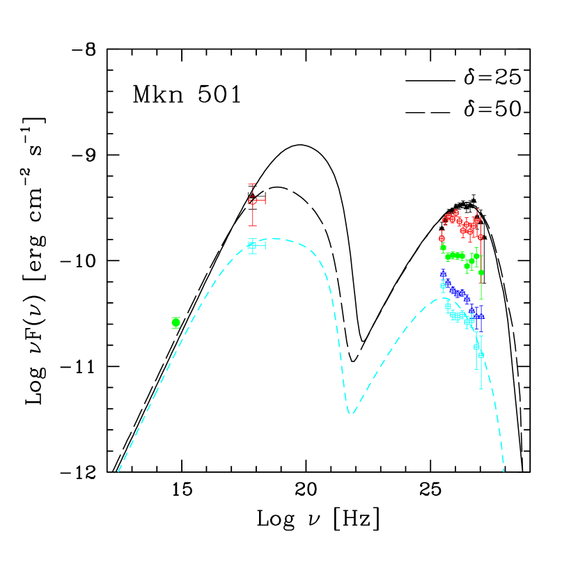
Figure 21: Overall SED from Mrk501. The optical data from the KVA Telescope is represented with a green full circle; the X-ray data from RXTE/ASM depicted with a black full triangle for June 30, red open circle for July 9, and light blue open square for the other nights (combined); the VHE data from MAGIC are represented as black full triangles (June 30), red open circles (July 9), green full circles (’high flux’ data-set), dark blue open triangles (’medium flux’ data-set), and light blue open squares (’low flux’ data-set). See Sect. 4.2 for definitions of high, medium and low flux data-sets. Vertical error bars denote 1$\sigma$ statistical uncertainties. The VHE spectra are corrected for EBL extinction using (Kneiske et al, 2004)’s ’Low’ EBL model. The highest and the lowest state were fit with a one zone SSC model (described in Tavecchio et al (2001)). See table 9 and section 5.5 for details of the modeling.

where $\eta\equiv\tau_{\rm syn}/\tau_{\rm IC}$, $\tau_{\rm syn}~{}=~{}E_{\rm e}^{\prime}/{\dot{P}}_{\rm syn}$, ${\dot{P}}_{\rm syn}=4\pi\sigma_{\rm T}cU_{\rm B}\gamma_{\rm e}^{2}/3$, $\sigma_{\rm T}$ is the Thomson cross section, $c$ the velocity of light, $U_{\rm B}=B^{2}/8\pi$ is the energy density of the magnetic field, $\gamma_{\rm e}=E_{\rm e}^{\prime}/mc^{2}$, and $m$ is the electron rest mass. The parameter $\eta$ corresponds to the ratio of the power emitted by electrons in IC and synchrotron processes, respectively (which is reciprocal to the coresponding cooling times $\tau_{\rm syn}/\tau_{\rm IC}$). The MAGIC $\gamma$-ray and corresponding RXTE/ASM X-ray data permit to constrain $\eta$ to $\lesssim$ 0.7. The modelling of the SED presented in section 5.5 (see, Fig. 21), however, suggests that $\eta$ is more likely of the order of $\sim 0.2$. We therefore used $\eta$=0.2 in all the following estimates. By comparing Eqs. 9,10 and 12 and setting $E_{\rm e}^{\prime}\approx E_{\rm TeV}/\delta$ TeV (where $\delta$ is the Doppler factor of the relativistically-moving emitting plasma blob and $E_{\rm TeV}$ is the electron energy (in TeV) in the observer’s frame, we obtain the condition on the acceleration efficiency of electrons,

$$\xi~{}\approx~{}10^{-3}BE_{\rm TeV}^{2}(1+\eta)\delta^{-2}.$$ (13)

If the observed decay timescale of the flare, $\tau_{\rm f}$, is also due to radiative processes, then,

$$\tau_{\rm cool}~{}=~{}\tau_{\rm f}\delta\,.$$ (14)

Inserting Eq. 12 into Eq. 14, and expanding $\tau_{\rm syn}$ and ${\dot{P}}_{\rm syn}$, permits to estimate $B$ in the cooling region:

$$B~{}\approx~{}11.2[(1+\eta)\cdot(E_{\rm TeV}\tau_{\rm f})]^{-1/2}~{}~{}~{}{\rm G},$$ (15)

with $\tau_{\rm f}$ in seconds. If electron acceleration and cooling are co-spatial, Eq. 13 becomes

$$\xi~{}\approx~{}1.1\times 10^{-2}{{E_{\rm TeV}^{3/2}\cdot(1+\eta)^{1/2}}\over{\tau_{\rm f}^{1/2}\delta^{2}}}$$ (16)

For the parameters of the July 9 flare Mrk501, the characteristic flux variability time $\tau_{\rm f}\approx 3$ minutes (see Sect. 3.3) and $E_{\rm TeV}\approx 1$, we obtain $B\approx 0.8$ G and $\xi\approx 0.9\times 10^{-3}\delta^{-2}$. Note, that this estimate of the magnetic field in the emission (acceleration) region of Mrk 501 is consistent with previous estimates, based on a homogeneous SSC model and the assumption of a very short variability timescale such as for the April 15-16 1997 flare (see e.g., Fig 3c in Bednarek & Protheore (1999)).

ii) Energy-dependent time delay in peak flare emission.

The time delay between the peaks of F($<$0.25 TeV) and F($>$1.2 TeV) during the July 9 flare, can be interpreted as due to the gradual acceleration of electrons in the relativistic blob. As reported in section 3.3, under the assumption that the shape of the flares is the same in the two energy ranges, the time delay is $\Delta\tau_{\rm H-L}=4\pm 1$ minutes.

Within the above framework, the time delay should correspond to the difference between the acceleration times of electrons to energies $E_{\rm TeV}^{\rm L}\approx 0.25$ and $E_{\rm TeV}^{\rm H}\approx 1.2$, according to

$$\tau_{\rm acc}^{\rm H}-\tau_{\rm acc}^{\rm L}~{}=~{}\Delta\tau_{\rm H-L}\delta.$$ (17)

Assuming for simplicity that the electron energies are determined by the energies of the emitted VHE radiation, i.e. ${E_{\rm e}^{{}^{\prime}{\rm L}}}$$\approx$$E_{\rm TeV}^{{}^{\prime}{\rm L}}/\delta$ and ${E_{\rm e}^{{}^{\prime}{\rm H}}}$$\approx$$E_{\rm TeV}^{{}^{\prime}{\rm H}}/\delta$, we can use Eq. 10 to model the acceleration time of electrons in eq.17. Finally, by reversing Eq. 17, we get another limit on the electron acceleration efficiency,

$$\xi~{}\approx~{}0.1{{(E_{\rm TeV}^{\rm H}-E_{\rm TeV}^{\rm L})}\over{B\delta^{2}\Delta\tau_{\rm H-L}}}.$$ (18)

Applying the observed values of $E_{\rm TeV}^{\rm H}$, $E_{\rm TeV}^{\rm L}$, $\Delta\tau_{\rm H-L}$ and the estimate of $B$ from Eq. 15 (which is valid if electron acceleration and cooling are co-spatial) we obtain $\xi$$\approx$$0.5\times 10^{-3}\delta^{-2}$, which is roughly the same value as determined above using the exponential flux decay time. Note that diffusion and/or spatial dishomogeneities might increase the volume where electrons cool down, thus making the magnetic field in the cooling region lower than that of the acceleration region. That would imply that the estimated values for the parameter $\xi$ using equations 16 and 18 are upper and lower limits, respectively.

We conclude that the time delay of the flare peak emission in different ranges of energy can result from the gradual acceleration of the emitting electrons in the blob. The inferred blazar Doppler factors, $\delta\sim 10-15$ (e.g. Costamante et al (2002)), imply a relatively inefficient acceleration, $\xi\sim 10^{-5}$. This value is significantly lower than required by the observations of $\gamma$-ray emission from the pulsar wind nebulae in which leptons are accelerated in the shock wave in the relativistic pulsar wind. For example, in the Crab Nebula $\xi$ has to be of the order of $\sim 0.1$, since leptons are accelerated clearly above $10^{3}$ TeV (approximately $10\%$ of the maximum available potential drop through the pulsar magnetosphere). Therefore, the physics of the acceleration process in the relativistic jets of BL Lacs and relativistic shocks in the pulsar wind nebulae may differ significantly.

A somewhat more speculative issue that blazar emission permits to explore concerns non-conventional physics. Energy-dependent arrival times are predicted by several models of Quantum Gravity, which quantify the first-order effects of the violation of Lorentz symmetry. One could, therefore, speculate that the observed time difference is explained by such models, although source-inherent effects could certainly not be excluded. A more detailed investigation of such interpretations of our data is still going on.

5.3 Interpretation of the spectral shape variations

The observed correlation between spectral shape and (bolometric) luminosity is naturally accounted for in the SSC scenario. Pian et al (1998); Tavecchio et al (2001) discuss the SED variations of Mrk 501 during the giant 1997 flare. During the 1997 flare the 0.1-200 keV band synchrotron spectrum became exceptionally flat (photon spectral index $a$$<$1), peaking at $\sim$$>$ 100 keV – a shift to higher frequencies by a factor of  100 from previous, more quiescent states. The VHE data (from the Whipple, HEGRA, and CAT telescopes) showed a progressive hardening from the baseline state ($a$$>$2) through a more active state to a flaring state ($a$$\sim$2). In the SSC scenario, these flux-dependent spectral changes implied that a drastic change in the electron spectrum caused the increase in emitted power: a freshly injected electron population has a flatter high-energy slope and a higher maximum energy than an aging population, which cause a shift of the SED to higher frequencies.

In section 4.4 we reported that the spectrum of Mrk 501 not only hardens on long time scales, with the overall emitted flux, but also during the shorter events of June 30 and July 9. The burst from July 9 showed a remarkable variability, and the evolution of the hardness ratio with the flux (right-hand plot of Fig 17) contains valuable information about the dynamics of the source. In the pre-burst phase, the hardness ratio does not vary significantly; yet during the burst phase, it varies following a clear loop pattern rotating counterclockwise. As pointed out by Kirk & Mastichiadis (1999), one expects to have this behaviour for a flare where the variability, acceleration and cooling timescales are similar; which implies that, during this flare, the dynamics of the system is dominated by the acceleration processes, rather than by the cooling processes. Consequently, the emission propagates from lower to higher energy, so the lower energy photons lead the higher energy ones (that is the so-called hard lag). This indeed agrees well with the argumentation given in section 5.2, where the time delay between $E_{>1.2~{}TeV}$ and $E_{<0.25~{}TeV}$ is shown to be consistent with the gradual acceleration of the electrons.

In a systematic study performed by Gliozzi et al (2006) using X-ray data from 1998 to 2004, this behaviour was not observed on more typical (longer) flares, where actually the opposite behaviour (clockwise rotation) was indicated. This might point to the fact that these physical processes might be responsible only for the shortest flux variations, and not for the variability on longer timescales.

5.4 Interpretation of the increased variability with energy

In the SSC framework, the variability observed in the VHE emission brings information about the dynamics of the underlying population of relativistic electrons (and possibly positrons). In this context, the general variability trend reported in section 3.4 is interpreted by the fact that the VHE $\gamma$-rays (as well as the X-rays) are produced by more energetic particles, that are characterized by shorter cooling timescales; causing the higher variability amplitude observed at the highest energies. It is worth noticing that such an injection of high energy particles would produce a shift in the IC peak, which is indeed observed during this observing campaign, as reported in sections 4 and 5.5.

5.5 Spectra corrected for the EBL absorption

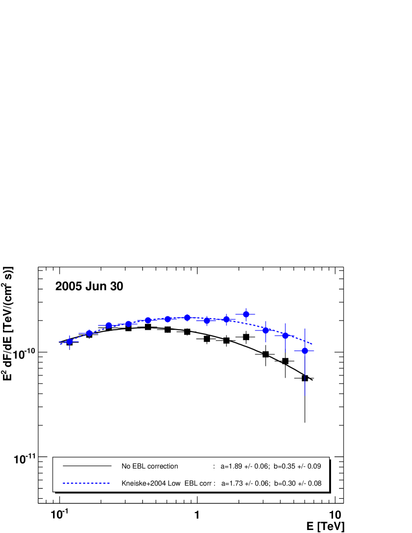
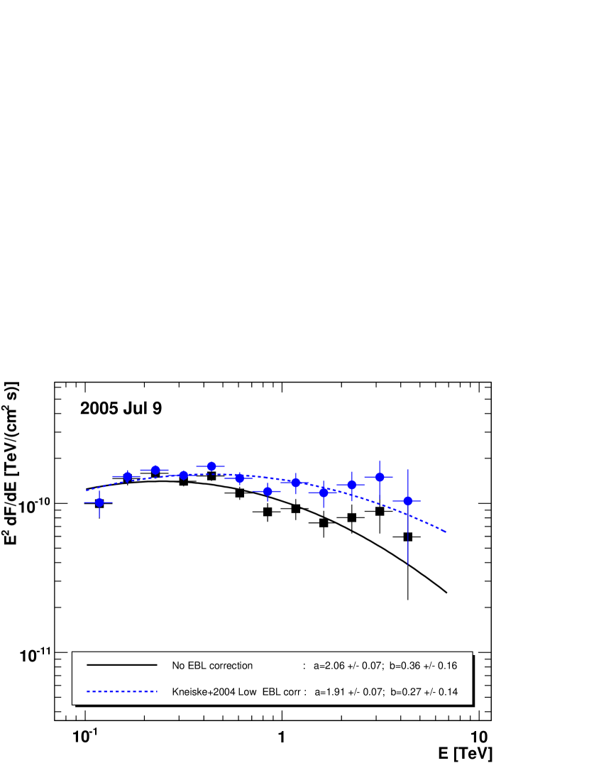
Figure 19: Spectra of Mrk 501 in the nights of June 30 (left) and July 9 (right) when the source was flaring. Bars as in Fig. 13. The spectra have been corrected for EBL absorption using (Kneiske et al, 2004)’s ’Low’ EBL model. The curves show log-parabolic fits (see eq. 6) whose corresponding parameters are reported in the insets.

In this section we correct the measured spectra for the EBL absorption. To this purpose we use Kneiske et al. (2004: ’Low’). A correction using the EBL models Aharonian et al. (2006) and and Primack et al. (2005) gave very similar results, while using Kneiske et al. (2004: ’Best’) and Stecker et al. (2006,2007) gave slightly larger energy fluxes above 1 TeV. Fig. 19 shows the spectra from the active nights June 30 and July 9 before/after correction for the EBL absorption. In spite of our proximity to Mrk501, the effect of the EBL is not negligible, and the spectral peak moves to higher energies.

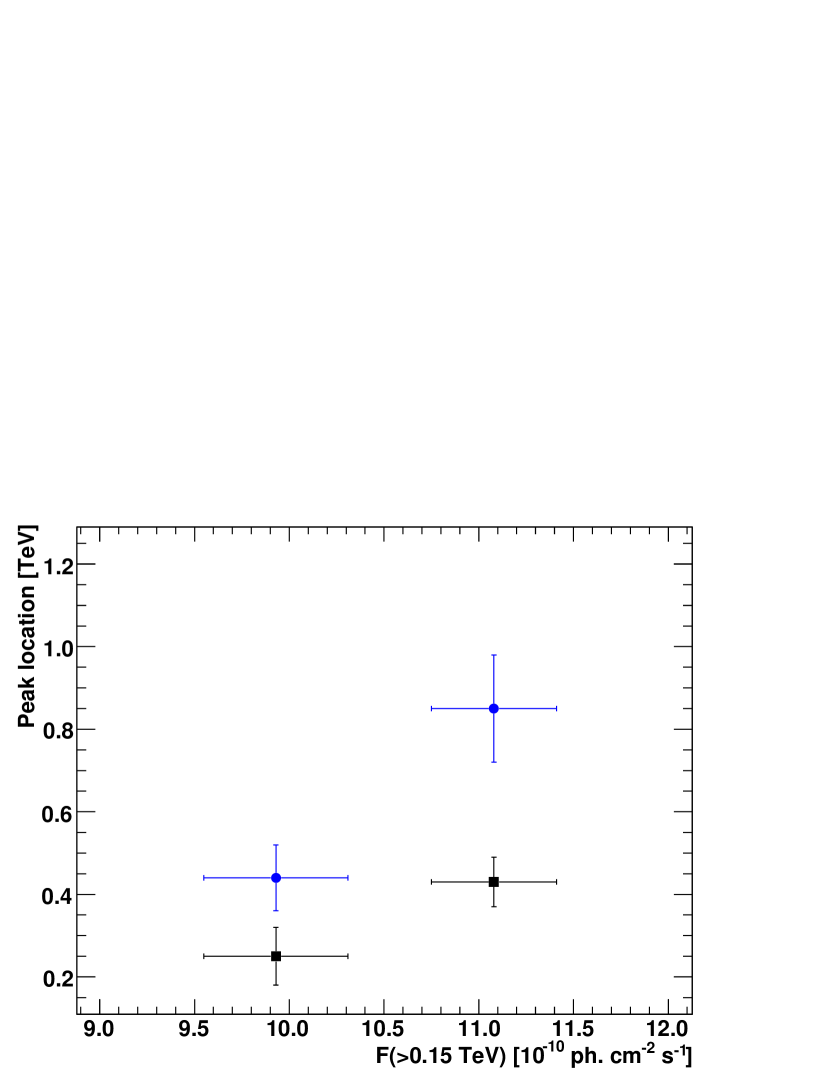
Figure 20: Spectral peak location versus flux above 0.15 TeV for the two flaring nights (June 30 and July 9). The spectra were fitted with eq. 6 (see Fig. 19) and the peak location and its associated error were calculated using eqs. 7 and 8. The black squares correspond to the observed spectra and the blue circles correspond to the spectra after correction for the EBL absorption using (Kneiske et al, 2004)’s ’Low’ EBL model.

The location of the spectral peaks (calculated using eqs. 7 and 8) are shown as a function of F ($>$0.15 TeV) in Fig. 20 for the flaring nights before and after the EBL correction. The figure seems to indicate a displacement of the peak location with the increasing flux, yet the error bars are too large to be conclusive. On the other hand the peak location is certainly at $<$0.1 TeV when Mrk 501 is in a low state (see sect. 4.2). Hence, there is evidence for an overall peak location versus luminosity trend.

Fig. 21 shows the June 30 and July 9 spectra, as well as the mean ’high’, ’medium’, and ’low’-flux spectra (see sect. 4.2), EBL-de-absorbed using the ’Low’ model of Kneiske et al (2004). The X-ray fluxes measured by RXTE/ASM, and the optical flux observed by the KVA Telescope, are also shown. The optical flux from the host galaxy, estimated by Nilsson et al (2007) to be 12.0 $\pm$ 1.2 mJy, has been subtracted.

The best-fitting one-zone, homogeneous SSC models of Mrk501’s intrinsic spectrum for the highest state of the source (corresponding to the active night of June 30) and for the lowest state (the mean spectrum corresponding to the ’low’-flux bin, see Fig. 13) are displayed in Fig. 21. The fit parameters (electron population’s break and max/min energies, high/low-$E$ spectral slopes, normalization: $E_{\rm br}$, $E_{\rm max}$, $E_{\rm min}$, $n_{1}$, $n_{2}$, $K$; plasma blob’s radius, magnetic field, Doppler factor $R$, $B$, $\delta$) are reported in Table 9 (see Tavecchio et al. 2001 for details on the model). It should be noted that two different fits to the high-state spectrum are possible – whose main differing parameters are, respectively, $\delta$,$B$=$25$, $0.23~{}G$ (solid black curve) and $50$, $0.053~{}G$ (dashed black curve) – which show that fairly different synchrotron peaks are possible within our X-ray and (EBL-corrected) TeV data. Spectrally more extended X-ray data would probably have solved the degeneracy. The optical data, too, do not lift the degeneracy: once the optical light contribution of the underlying host galaxy is subtracted, the observed energy flux is rather compatible with the SED models for the different activity states. The fit to the ’low’-state spectrum is characterized, perhaps unsurprisingly, by a change of the internal physical conditions of the emitting plasma blob rather than by a change of its bulk attributes (blob size and relativistic Doppler factor): the low state is characterized, with respect to the high state, by lower max/break energies and normalization of the electron population and by a somewhat stronger magnetic field. One nice consistency feature of all the fits is that, in all cases, the radius of the plasma blob, $R$$=$$10^{15}$ cm, implies a crossing time $t_{\rm cr}$$=$$R/\delta c$, comparable to that inferred from the observed duration ($\sim$20 minutes) of the flare, $\Delta$$t_{\rm flare}$.

The SED models for Mrk 501 derived and discussed in this section can be compared with some previous published models, like Pian et al. (1998): $\delta,B$$\simeq$$15,0.8$G from one-zone SSC modeling of 1997 SEDs, with flatter/steeper electron distributions for active/quiescent phases; Tavecchio et al. (1998): $\delta,B$$\simeq$$8-20,0.5-1$G from one-zone SSC modeling of historical quiescent SED and $\delta,B$$\simeq$$7,1$G (and very high break energy) for the active SED; Bednarek & Protheroe (1999): $\delta,B$$\simeq$$12-36,0.07-0.6$G from 1997 SEDs modeled with one-zone SSC requiring $\gamma$-ray  transparency of the emitting blob; Kataoka et al. (1999): $\delta,B$$\simeq$$15,0.2$G from one-zone SSC modeling of simultaneous 1996 SED; Katarzyński et al. (2001): $\delta,B=14,0.2$G from SSC modeling of non-simultaneous broadband SED. The SED of Mrk 501 can also be modelled by less conventional approaches, requiring magnetic fields in the emission region smaller than $0.005$G, Krawczynski (2007). We should, however, remember that for this highly variable source, constraints derived for some epochs may not apply to other epochs (the simple one-zone model has 9 free parameters!): in particular, most published models refer to the giant 1997 flare hence comparisons with our results may not be straightforward. However, Tavecchio et al. (2001) modelled different emission states of Mrk501 in 1997, 1998, and 1999 by just changing the electron energy distribution (slopes, break energy, number density) and keeping the other parameters frozen, similarly to what was done here (see in Table 9 the two states represented by solid lines in Fig. 21). It is also worth mentioning the work done by Krawczynski et al (2002), in which the energy spectra (for different days) were modelled using a time-dependent code.

It should be remarked that in TeV blazars, while the bright and rapidly variable VHE emission implies that at the scales where this emission originates ($\sim$0.1 pc from the jet apex) the jet is highly relativistic ($\delta$$\sim$10-20 with no EBL-absorption correction, and $\delta$$\sim$$<$ 50 with correction), at VLBI ($\sim$1 pc) scales the jets are relatively slow (see Ghisellini et al. 2005, and references therein). Hence, to reconcile the high $\delta$’s derived from VHE data with the much lower $\delta$’s derived from VLBI radio measurements, the jets of TeV blazars must either undergo severe deceleration (Georganopoulos & Kazanas 2003) or be structured radially as a two-velocity, inner spine plus outer layer, flow (Ghisellini et al. 2005).

6 Concluding remarks

In this work, we have undertaken a systematic study of the temporal and spectral variability of the nearby blazar Mrk 501 with the MAGIC telescope at energies $>$ 0.1 TeV. During 24 observing nights between May and July 2005, all of which yielded significant detections, we measured fluxes and spectra at levels of baseline activity ranging from $<$0.5 to $>$1 c.u.. During two nights, on June 30 and July 9, Mrk 501 underwent into a clearly active state with a $\gamma$-ray emission $>$3 c.u., and flux-doubling times of $\sim$2 minutes. The $\sim$20-minute long flare of July 9 showed an indication of a 4$\pm$1 min time delay between the peaks of F($<$0.25 TeV) and F($>$1.2 TeV), which may indicate a progressive acceleration of electrons in the emitting plasma blob. An overall trend of harder spectra for higher flux is clearly seen on intra-night, night-by-night, and longer-term timescales. The VHE $\gamma$-ray variability was found to increase with energy, regardless whether the source is in active or quiescent state, and it is significantly higher than the variability at X-ray frequencies. A spectral peak, at a location dependent on source luminosity, was clearly observed during the active states. All these features are naturally expected in synchro-self-Compton (SSC) models of blazar VHE emission. There are no simultaneous good quality X-ray measurements during the MAGIC observations. As a consequence, the SSC model of the X-ray/VHE SED of Mrk 501 in an active state is not unequivocally constrained, but it still restricts the emitting plasma blob to have Doppler factors in range of 25-50 and magnetic fields in the range 0.05-0.5 G.

7 Acknowledgments

We would like to thank the IAC for the excellent working conditions on the La Palma Observatory Roque de los Muchachos. We are grateful to the ASM/RXTE team for their quick-look results. The support of the German BMBF and MPG, the Italian INFN and the Spanish CICYT is gratefully acknowledged. This work was also supported by ETH Research Grant TH-34/04-3 and by Polish Grant MNiI 1P03D01028. Besides, the authors want to thank Deirdre Horan, Martin Tluczykont and Frédéric Piron for providing Mrk501 data from WHIPPLE, HEGRA CT1, HEGRA CT System and CAT, respectively, and for useful discussions.

Table 1: MAGIC observation of Mrk 501

MJD	$T_{obs}$	ZA	$S_{comb}$	$F_{>0.15~{}TeV}$	$F_{>0.15~{}TeV}$	$K_{0}$	$a$	${\chi^{2}}/{NDF}$	$P$
Start	($h$)	($deg$)	sigma	($\frac{10^{-10}~{}ph}{cm^{2}\cdot s}$)	(Crab Units)	($\frac{10^{-10}~{}ph}{cm^{2}\cdot s\cdot 0.3TeV}$)			(%)
53518.980	0.75	19.10-28.95	6.44	1.19 $\pm$ 0.25	0.37 $\pm$ 0.08	2.63 $\pm$ 0.48	2.17 $\pm$ 0.25	2.7/8	95.2
53521.966	1.85	9.97-30.10	8.90	1.51 $\pm$ 0.17	0.47 $\pm$ 0.05	2.94 $\pm$ 0.33	2.61 $\pm$ 0.16	10.8/7	15.0
53524.969	0.58	19.18-27.73	6.98	2.04 $\pm$ 0.29	0.64 $\pm$ 0.09	3.71 $\pm$ 0.53	2.47 $\pm$ 0.23	1.6/6	95.0
53526.975	0.98	9.96-28.94	8.69	1.63 $\pm$ 0.22	0.51 $\pm$ 0.07	3.26 $\pm$ 0.38	2.49 $\pm$ 0.17	3.8/9	92.4
53530.973	0.47	15.22-22.32	6.52	1.53 $\pm$ 0.32	0.48 $\pm$ 0.10	2.28 $\pm$ 0.65	1.97 $\pm$ 0.49	1.1/3	78.9
53531.959	0.90	15.21-25.15	6.98	1.29 $\pm$ 0.24	0.41 $\pm$ 0.07	2.69 $\pm$ 0.38	2.57 $\pm$ 0.30	9.1/6	16.6
53532.936	0.53	23.80-30.11	5.44	1.50 $\pm$ 0.28	0.47 $\pm$ 0.09	2.41 $\pm$ 0.53	2.34 $\pm$ 0.36	1.2/7	99.2
53533.933	1.63	12.85-30.09	7.83	1.44 $\pm$ 0.17	0.45 $\pm$ 0.05	2.46 $\pm$ 0.32	2.55 $\pm$ 0.19	10.3/8	24.2
53534.940	2.07	9.95-30.09	9.56	1.43 $\pm$ 0.15	0.45 $\pm$ 0.05	2.71 $\pm$ 0.27	2.68 $\pm$ 0.16	8.9/9	44.8
53535.934	3.43	9.95-30.07	18.58	2.69 $\pm$ 0.13	0.85 $\pm$ 0.04	4.45 $\pm$ 0.24	2.42 $\pm$ 0.06	11.9/12	45.3
53536.947	2.68	9.95-29.93	7.01	0.75 $\pm$ 0.13	0.24 $\pm$ 0.04	1.36 $\pm$ 0.21	2.73 $\pm$ 0.29	5.7/7	57.1
53537.971	3.08	9.95-30.10	11.52	1.25 $\pm$ 0.10	0.39 $\pm$ 0.03	2.08 $\pm$ 0.19	2.46 $\pm$ 0.14	8.2/8	41.4
53548.931	0.87	9.98-20.68	6.12	1.21 $\pm$ 0.25	0.38 $\pm$ 0.08	2.39 $\pm$ 0.38	2.28 $\pm$ 0.27	0.6/6	99.6
53551.905	1.09	12.86-25.15	32.02	11.08 $\pm$ 0.32	3.48 $\pm$ 0.10	17.37 $\pm$ 0.51	2.09 $\pm$ 0.03	26.2/11	0.6
53554.906	0.68	15.21-22.32	12.52	3.52 $\pm$ 0.30	1.11 $\pm$ 0.09	5.91 $\pm$ 0.47	2.26 $\pm$ 0.11	3.9/9	92.1
53555.914	0.44	12.85-22.32	6.08	1.27 $\pm$ 0.34	0.40 $\pm$ 0.11	2.96 $\pm$ 0.62	1.97 $\pm$ 0.29	1.9/6	92.5
53557.916	0.54	12.84-19.06	8.40	2.25 $\pm$ 0.32	0.71 $\pm$ 0.10	3.91 $\pm$ 0.48	2.30 $\pm$ 0.21	6.5/7	48.5
53559.920	0.98	9.94-17.22	10.05	1.85 $\pm$ 0.23	0.58 $\pm$ 0.07	3.10 $\pm$ 0.33	2.25 $\pm$ 0.13	8.4/8	39.9
53560.906	0.76	9.96-19.07	24.39	9.93 $\pm$ 0.38	3.12 $\pm$ 0.12	14.35 $\pm$ 0.56	2.20 $\pm$ 0.04	22.5/11	2.1
53562.911	1.63	9.94-16.79	11.08	2.19 $\pm$ 0.37	0.69 $\pm$ 0.12	2.83 $\pm$ 0.30	2.34 $\pm$ 0.13	14.1/8	8.2
53563.921	0.85	9.94-15.16	18.69	5.53 $\pm$ 0.28	1.74 $\pm$ 0.09	7.89 $\pm$ 0.39	2.25 $\pm$ 0.06	11.5/9	24.3
53564.917	0.34	9.94-15.18	8.91	2.89 $\pm$ 0.46	0.91 $\pm$ 0.15	4.88 $\pm$ 0.56	2.27 $\pm$ 0.20	5.4/6	49.7
53565.920	2.57	9.95-28.93	11.62	1.71 $\pm$ 0.13	0.54 $\pm$ 0.04	2.73 $\pm$ 0.22	2.49 $\pm$ 0.12	10.7/8	21.6
53566.953	1.91	9.99-30.10	11.63	1.33 $\pm$ 0.11	0.42 $\pm$ 0.04	2.16 $\pm$ 0.20	2.28 $\pm$ 0.13	7.4/10	69.0

Table 2: Flare model parameters: integral emission above 0.15 TeV.

Date	$T_{obs}$	$S_{comb}$	$a$	$a$	$b$	$c$	$d$	${\chi^{2}}/{NDF}$	$P$
	($h$)	(sigma)	($\frac{10^{-10}~{}ph}{cm^{2}\cdot s}$)	(Crab Units)	($\frac{10^{-10}~{}ph}{cm^{2}\cdot s}$)	$(s)$	$(s)$		(%)
June 30	0.63	24.7	10.80$\pm$0.48	3.39$\pm$0.15	13.2$\pm$4.7	81$\pm$41	50$\pm$23	20.0/15	17.3
July 9	0.36	19.6	7.39$\pm$0.48	2.32$\pm$0.15	20.3$\pm$3.3	95$\pm$24	185$\pm$40	4.2/7	75.8

Table 3: Flare model parameters for June 30: differential emission.

Energy Range	$a$	$a$	$b$	$c$	$d$	${\chi^{2}}/{NDF}$	$P$
(TeV)	($\frac{10^{-10}~{}ph}{cm^{2}\cdot s}$)	(Crab Units)	($\frac{10^{-10}~{}ph}{cm^{2}\cdot s}$)	$(s)$	$(s)$		(%)
0.25-0.6	3.30$\pm$0.23	3.0$\pm$0.2	7.5$\pm$2.8	110$\pm$57	61$\pm$26	5.2/6	51.8

Table 4: Flare model parameters for July 9 resulting from a combined fit to all LCs from Fig. 7 using equation 2 with c=d. The overall ${\chi^{2}}/{NDF}$ = 14.0/12 ($P$=0.3)

Energy Range	$a$	$a$	$b$	$c$	$t_{0}-t_{0}^{LC~{}E~{}0.15-0.25TeV}$
(TeV)	($\frac{10^{-10}~{}ph}{cm^{2}\cdot s}$)	(Crab Units)	($\frac{10^{-10}~{}ph}{cm^{2}\cdot s}$)	$(s)$	$(s)$
0.15-0.25	4.23$\pm$0.49	2.48$\pm$0.28	8.6$\pm$3.7	143$\pm$92	0 $\pm$ 68
0.25-0.6	2.55$\pm$0.24	2.32$\pm$0.09	9.3$\pm$2.5	95$\pm$28	7 $\pm$ 36
0.6-1.2	0.53$\pm$0.10	1.96$\pm$0.37	2.7$\pm$0.9	146$\pm$56	111 $\pm$ 91
1.2-10	0.23$\pm$0.06	1.51 $\pm$0.39	4.0$\pm$0.9	103$\pm$19	239 $\pm$ 40

Table 5: Flare model parameters for July 9 resulting from a combined fit to all LCs from Fig. 8 using equation 2 with $c=d$, and with a common $t_{0}$ for all LCs. The overall ${\chi^{2}}/{NDF}$ = 25.6/15 ($P$=0.04)

Energy Range	$a$	$a$	$b$	$c$	$t_{0}-t_{0}^{LC~{}E~{}0.15-0.25TeV}$
(TeV)	($\frac{10^{-10}~{}ph}{cm^{2}\cdot s}$)	(Crab Units)	($\frac{10^{-10}~{}ph}{cm^{2}\cdot s}$)	$(s)$	$(s)$
0.15-0.25	4.23$\pm$0.49	2.48$\pm$0.28	5.4$\pm$2.2	301$\pm$210	0 $\pm$ 42
0.25-0.6	2.55$\pm$0.24	2.32$\pm$0.09	5.7$\pm$1.5	162$\pm$63	0 $\pm$ 42
0.6-1.2	0.53$\pm$0.10	1.96$\pm$0.37	2.6$\pm$0.8	153$\pm$56	0 $\pm$ 42
1.2-10	0.23$\pm$0.06	1.51 $\pm$0.39	3.9$\pm$1.0	97$\pm$22	0 $\pm$ 42

Table 6: Stacked analysis: mean spectral parameters.

Flux Level	$T_{obs}$	ZA	$S_{comb}$	$F_{>0.15~{}TeV}$	$F_{>0.15~{}TeV}$	$K_{0}$	$a$	${\chi^{2}}/{NDF}$	$P$
	($h$)	($deg$)	sigma	($\frac{10^{-10}~{}ph}{cm^{2}\cdot s}$)	(Crab Units)	($\frac{10^{-10}~{}ph}{cm^{2}\cdot s\cdot 0.3TeV}$)			(%)
$Low$	17.2	9.96-30.1	16.7	1.24$\pm$ 0.08	0.39 $\pm$ 0.02	2.31$\pm$0.13	2.45 $\pm$ 0.07	7.8/7	34.6
$Medium$	11.0	9.95-30.0	22.8	2.11$\pm$ 0.09	0.66 $\pm$ 0.03	3.57$\pm$0.15	2.43 $\pm$ 0.05	2.9/7	89.4
$High$	1.52	9.95-22.3	21.7	4.62$\pm$ 0.21	1.45 $\pm$ 0.07	7.13$\pm$0.32	2.28 $\pm$ 0.05	4.8/7	68.7

Table 7: PL (eq. 5) and Log-parabolic (eq. 6) fit results for June 30 and July 9: night-integrated spectra.

	Fit performed with eq. 5				Fit performed with eq. 6
Date	$K_{0}$	$a$	${\chi^{2}}/{NDF}$	$P$	$K_{0}$	$a$	$b$	${\chi^{2}}/{NDF}$	$P$
	($\frac{10^{-10}~{}ph}{cm^{2}\cdot s\cdot 0.3TeV}$)			(%)	($\frac{10^{-10}~{}ph}{cm^{2}\cdot s\cdot 0.3TeV}$)				(%)
June 30	17.4$\pm$0.05	2.09$\pm$0.03	26.1/11	0.6	18.6$\pm$0.06	1.89$\pm$0.06	0.35$\pm$0.09	6.1/10	80.1
July 9	14.3$\pm$0.06	2.20$\pm$0.04	22.5/11	2.1	15.5$\pm$0.07	2.06$\pm$0.07	0.36$\pm$0.16	15.2/10	12.5

Table 8: Log-parabolic (eq. 6) fit results for June 30 and July 9, 2005: pre-burst and burst spectra.

MJD	$T_{obs}$	$S_{comb}$	$F_{>0.15~{}TeV}$	$F_{>0.15~{}TeV}$	$K_{0}$	$a$	$b$	${\chi^{2}}/{NDF}$	$P$
Start	($h$)	sigma	($\frac{10^{-10}~{}ph}{cm^{2}\cdot s}$)	(Crab Units)	($\frac{10^{-10}~{}ph}{cm^{2}\cdot s\cdot 0.3TeV}$)				(%)
53551.905	0.46	22.3	10.99$\pm$0.48	3.46$\pm$0.15	19.8$\pm$1.0	1.97$\pm$0.08	0.27$\pm$0.14	8.2/9	51.2
53551.924	0.63	24.7	11.15$\pm$0.43	3.50$\pm$0.14	17.2$\pm$0.8	1.87$\pm$0.08	0.34$\pm$0.13	13.8/10	18.1
53560.906	0.40	15.2	7.64 $\pm$ 0.48	2.40 $\pm$ 0.15	12.7$\pm$1.1	2.11$\pm$0.12	0.57$\pm$0.34	6.4/8	59.8
53560.923	0.36	19.6	12.39 $\pm$ 0.60	3.89 $\pm$ 0.19	19.3$\pm$1.3	2.00$\pm$0.10	0.44$\pm$0.23	8.9/8	35.2

Table 9: SSC model parameters

spectrum	$\gamma_{\rm min}$	$\gamma_{\rm br}$	$\gamma_{\rm max}$	n1	n2	B	K	R	Doppler factor
						Gauss	particle/$cm^{3}$	cm
June 30	1	$10^{6}$	$10^{7}$	2	3.5	0.23	7.5$\cdot$ $10^{4}$	$10^{15}$	25
June 30 (bis)	1	$5\cdot 10^{5}$	$10^{7}$	2	3.5	0.053	7.0$\cdot$ $10^{4}$	$10^{15}$	50
Low flux	1	$10^{5}$	$5\cdot 10^{6}$	2	3.2	0.31	4.3$\cdot$ $10^{4}$	$10^{15}$	25

Figure 8: Same as in figure 7, but with a common T0 (which was also fit) for all LCs. The resulting parameters from this combined fit are reported in table 5.

References

- Aharonian et al (1999a) Aharonian et al 1999a, A&A, 342, 69
- Aharonian et al (1999b) Aharonian et al 1999b, A&A, 349, 11
- Aharonian et al (2000) Aharonian F. A. 2000, New Astr. Rev., 5, 377
- Aharonian et al (2001) Aharonian et al 2001, ApJ, 546, 898
- Aharonian et al (2003) Aharonian et al 2003, A&A, 403, L1
- Aharonian et al (2004) Aharonian et al 2004, ApJ 614, 897
- Aharonian et al (2006) Aharonian, F. et al 2006, Nature, 440, 1018
- Aharonian et al (2006) Aharonian et al 2006, Science, 314, 1424 (2006)
- Aharonian et al (2007) Aharonian et al 2007, in press, arXiv:0706.0797
- Albert et al (2006) Albert et al 2006, astro-ph/0612385
- Amelino-Camelia et al (1998) Amelino-Camelia, G., et al 1998, Nature 393, 763
- Anykeyev et al (1991) Anykeyev, V.B. et al 1991, Nucl. Instr. Meth. A, 303, 350
- Atoyan et al (2003) Atoyan, A.M., & Dermer, C.D. 2003, ApJ, 586, 79
- Baixeras et al (2004) Baixeras, C. et al 2004, Nucl. Instr. Meth. A, 518, 188
- Bassani & Dean (1981) Bassani, L., & Dean, J. 1981, Nature 294, 332
- Barrio et al (1998) Barrio, J.A. et al 1998, The MAGIC Telescope, 1998
- Beall & Bednarek (1999) Beall, J.H., & Bednarek W. 1999, ApJ, 510, 188
- Bednarek (1993) Bednarek, W. 1993, ApJ, 402, L29
- Bednarek et al (1996) Bednarek, W., et al 1996, A&A, 307, L17
- Bednarek & Protheore (1997a) Bednarek, W., & Protheroe, R.J. 1997a, MNRAS, 287, L9
- Bednarek & Protheore (1997b) Bednarek, W., & Protheroe, R.J. 1997b, MNRAS, 290, 139
- Bednarek & Protheore (1999) Bednarek, W., & Protheroe, R.J. 1999, MNRAS, 310, 577
- Bertero (1989) Bertero, M. 1989, Advances in Electronics and Electron Physics, Vol. 75, Academic Press 1989.
- Bityukov et al (2006) Bityukov S. et al, http://arxiv.org/abs/physics/0612178v3
- Blandford & Rees (1978) Blandford R. D., & Rees M. J. 1978, in Proc. Pittsburgh Conference on BL Lac Objects, ed. A. Wolfe (Univ. Pittsburgh Press), 328
- Blandford & Königl (1979) Blandford, R.D., & Königl 1979, A., ApJ, 232, 34
- Böttcher (2002) Böttcher M. 2002, in Proc. XXII Moriond Astrophsics Meeting ’The Gamma-ray Universe’, 151
- Bradbury et al (1997) Bradbury, S.M. et al 1997, A&A 320, L5
- Catanese et al (1997) Catanese, M., et al 1997, ApJ, 487, L143
- Coppi et al (1993) Coppi, P.S., Kartje, J.F., & Koenigl, A. 1993, in Proc. Compton GRO Symp., AIP 280, 559
- Cortina et al (2005) Cortina, J. et al 2005, in Proc. 29th International Cosmic Ray Conference, Pune (India), astro-ph/0508274
- Costamante et al (2002) Costamante, L., & Ghisellini, G. 2002, A&A, 384, 56
- Dar & Laor (1997) Dar, A., & Laor, A. 1997, ApJ, 478, L5
- Dermer & Schlickeiser (1993) Dermer, C.D., & Schlickeiser, R. 1993, ApJ, 416, 458
- Djanati-Ataïet al (1999) Djanati-Ataï, A., et al1999, A&A 350, 17
- Dondi & Ghisellini (1995) Dondi, L. & Ghisellini, G. 1995, MNRAS, 273, 583
- Edelson et al (2002) Edelson R., et al. 2002, ApJ, 568, 610
- Ellis et al (2006) Ellis, G., et al 2006, Astropart. Phys., 25, 402
- Ferenc & Hrupec (2007) Ferenc, D., & Hrupec, D. 2007, in preparation
- Fossati et al (1998) Fossati, G. et al 1998, MNRAS, 299, 433
- Gaidos (1996) Gaidos, J.A. et al 1996, Nature 383, 319
-
Gaug (2006)
Gaug M. 2006, PhD Thesis, IFAE Barcelona
http://wwwmagic.mppmu.mpg.de/publications/theses/ - Georganopoulos & Kazanas (2003) Georganopoulos, M., & Kazanas, D. 2003, ApJ, 594, L27
- Ghisellini & Madau (1996) Ghisellini, G., & Madau, P. 1996 MNRAS, 280, 67
- Ghisellini et al (1998) Ghisellini, G., Celotti, A., Fossati, G. et al 1998, MNRAS, 299, 453
- Ghisellini et al (2005) Ghisellini, G., Tavecchio, F., & Chiaberge, M. 2005, A&A, 432, 401
- Gliozzi et al (2006) Gliozzi, M. et al 2006, ApJ, 646, 61
- Hayashida et al (1998) Hayashida, N., et al 1998, ApJ, 504, L71
- Henri et al (1993) Henri, G., Pelletier, G., & Roland, J. 1993, ApJ, 404, L41
- Hillas (1985) Hillas, A.M. 1985, in Proc. 19th International Cosmic Ray Conference, La Jolla
- Hillas et al (1998) Hillas et al 1998, ApJ 503, 744
- Kataoka et al (1999) Kataoka, J., et al 2001, ApJ, 514, 138
- Katarzyński et al (2001) Katarzyński, K., Sol, H., & Kus, A. 2001, A&A, 367, 809
- Krawczynski et al (2002) Krawczynski, H., Coppi, P. S., Aharonian, F., 2002, MNRAS, 336, 721
- Krawczynski et al (2004) Krawczyński, K., et al 2004, ApJ, 601, 151
- Krawczynski (2007) Krawczynski, H., 2007, in press [astro-ph/0610641]
- Hrupec (2007) Hrupec, D. 2007, PhD Thesis, University of Zagreb
- Kirk & Mastichiadis (1999) Kirk, J.G., & Mastichiadis, A. 1999, in ’TeV Astrophysics of Extragalactic Sources’ (eds. M.Catanese & T.Weekes), Astropart. Phys., 11, 45
- Kneiske et al (2004) Kneiske, T. M., et al 2004, A&A, 413, 807
- Kranich (2000) Kranich, D. 2000, PhD Thesis, MPI Munich
- Li & Ma (1983) Li, T. & Ma, Y. 1983, ApJ, 272, 317
- Lorenz et al (1995) Lorenz, E. et al 1995, in Proc. ’Towards a Major Atmospheric Cherenkov Detector IV’, Padova Univ
- Lyutikov (2003) Lyutikov, M. 2003, New Astr. Rev., 47, 513
- Mannheim & Biermann (1992) Mannheim, K., & Biermann, P.L. 1992, A&A, 253, L21
- Mannheim (1993) Mannheim, K. 1993, A&A 269, 67
- Maraschi et al (1992) Maraschi, L., Ghisellini, G., Celotti, A. 1992, ApJ, 397, L5
- Maraschi et al (1999) Maraschi, L. et al 1999, Astropart. Phys., 11, 189
- Marscher et al (1985) Marscher, A.P., & Gear, W.K. 1985, ApJ, 298, 11
- Massaro et al (2004) Massaro, E. et al 2004, A&A 413, 489
- Massaro et al (2006) Massaro, E. et al 2006, A&A 448, 861
- Mastichiadis & Kirk (1997) Mastichiadis, A., & Kirk, K.J. 1997, A&A, 320, 19
- Mattox et al (1993) Mattox, J.R., et al 1993, ApJ, 410, 609
- McBreen (1979) McBreen, B., 1979, AA, 71, L17
- Multi-Messenger-Group (2006) Multi-Messenger-Group, http://www-zeuthen.desy.de/multi-messenger/GammaRayData/index.html
- Mücke et al (2003) Mücke, A. et al 2003, Astropart. Phys., 18, 593
- Nandra et al (1997) Nandra, K., et al 1997, ApJ, 476, 70
- Nilsson et al (2007) Nilsson, K. et al 2007, in press, arXiv:0709.2533
- Osone (2006) Osone S. 2006, Astropart. Phys. 26, 209
-
Paneque (2004)
D. Paneque, 2004, PhD Thesis, MPI Munich
http://wwwmagic.mppmu.mpg.de/publications/theses - Petry et al (1996) Petry, D. et al 1996, A&A, 311, L13
- Pian et al (1998) Pian, E., et al 1998, ApJ, 492, L17
-
Piron (2000)
Piron, F. 2000, PhD Thesis,
http://lpnp90.in2p3.fr/ cat/Thesis - Piron (2001) Piron, F. 2001, in Proc. XXXVI Rencontres de Moriond ’Very High-Energy Phenomena in the Universe’, astro-ph/0106210
- Poe et al (2005) Poe, G.L., Giraud, K.L., & Loomis, J.B, Am. J. Agricultural Economics, 87 (2), 353 (2005)
- Pohl & Schlieckeiser (2000) Pohl, M. & Schlieckeiser, R. 2000, A&A, 354, 395
- Primak et al (2005) Primack, J., et al 2005, AIP Conf. Proc., 745, 23
- Punch et al (1992) Punch, M., et al 1992, Nature 358, 477
- Quinn et al (1996) Quinn, J., et al 1996, ApJ 456, L83
- Quinn et al (1999) Quinn, J., et al 1999, ApJ, 518, 693
- Ravasio et al (2004) Ravasio, M., et al 2004, A&A 424, 841
- Rees (1978) Rees, M.J. 1978, MNRAS, 184, P61
- Rees (1984) Rees, M.J. 1984, ARA&A, 22, 471
- Rieger & Mannheim (2000) Rieger, F.M., & Mannheim, K. 2000, A&A 359, 948
- Rieger & Mannheim (2002) Rieger, F.M.., & Mannheim, K. 2003, A&A 397, 121
- Samuelson et al (1998) Samuelson et al 1998, ApJ, 501, L17
-