Predicted and observed evolution in the mean properties of Type Ia supernovae with redshift

Abstract

Recent studies indicate that Type Ia supernovae (SNe Ia) consist of two groups — a “prompt” component whose rates are proportional to the host galaxy star formation rate, whose members have broader lightcurves and are intrinsically more luminous, and a “delayed” component whose members take several Gyr to explode, have narrower lightcurves, and are intrinsically fainter. As cosmic star formation density increases with redshift, the prompt component should begin to dominate. We use a two-component model to predict that the average lightcurve width should increase by 6% from $z=0-1.5$. Using data from various searches we find an 8.1%$\pm$2.7% increase in average lightcurve width for non-subluminous SNe Ia from $z=0.03-1.12$, corresponding to an increase in the average intrinsic luminosity of 12%. To test whether there is any bias after supernovae are corrected for lightcurve shape we use published data to mimic the effect of population evolution and find no significant difference in the measured dark energy equation of state parameter, $w$. However, future measurements of time-variable $w$ will require standardization of SN Ia magnitudes to 2% up to $z=1.7$, and it is not yet possible to assess whether lightcurve shape correction works at this level of precision. Another concern at $z=1.5$ is the expected order of magnitude increase in the number of SNe Ia that cannot be calibrated by current methods.

1. Introduction

Type Ia supernovae (SNe Ia) are the most important standardized candles for cosmology, and have been used to discover dark energy and the accelerating universe (Riess et al., 1998; Perlmutter et al., 1999). This was facilitated by the realization that supernovae with broader lightcurves are intrinsically brighter, while those with narrow lightcurves are dimmer (Phillips, 1993). Various schemes exist to correct SN Ia luminosities based on their lightcurve shape (e.g. Riess, Press, & Kirshner, 1996; Tonry et al., 2003; Prieto, Rest, & Suntzeff, 2006; Guy et al., 2007; Jha, Riess, & Kirshner, 2007) — here we use the “stretch” method, in which the time axis of a template lightcurve is multiplied by a scale factor $s$ to fit the data (Perlmutter et al., 1997).

Some properties of SNe Ia have been found to correlate with environment — brighter supernovae with broader lightcurves (high $s$) tend to occur in late-type spiral galaxies (Hamuy et al., 1995), while dimmer, fast declining (low $s$) supernovae are preferentially located in an older stellar population, leading to the conclusion that the age of the progenitor system is a key variable affecting SN Ia properties (Howell, 2001). The fact that supernovae occur at a much higher rate in late type galaxies, and that the SN Ia rate is proportional to the core-collapse rate (Mannucci et al., 2005) is another indication that age plays an essential role. Following this previous work, Scannapieco & Bildsten (2005) model SNe Ia as consisting of two populations — a “prompt” component whose rate is proportional to the star formation rate of the host galaxy, and a second “delayed” component whose rate is proportional to the stellar mass of the galaxy. Sullivan et al. (2006, hereafter S06) tie all of these results together using data from the Supernova Legacy Survey (SNLS), finding that slow declining, brighter SNe Ia come from a young population and have a rate proportional to star formation on a 0.5 Gyr timescale, while dimmer, faster declining supernovae come from a much older population with a rate proportional to the mass of the host galaxy.

S06 and Mannucci, Della Valle, & Panagia (2006) predict that the SNe Ia whose rates are proportional to star formation will start to dominate the total sample of SNe as cosmic star formation increases with redshift. Since these SNe are intrinsically brighter, the mean luminosity of the population should increase with redshift. Here we use the two-component SN Ia model of Scannapieco & Bildsten (2005) and the stretch distribution for each component from SNLS data (S06) to quantify the expected magnitude of this effect. We then compare the predicted evolution in lightcurve stretch to SN distributions from the SNLS and the Higher-z SN Search (Riess et al., 2007).

2. Predicting Evolution

Scannapieco & Bildsten (2005) parameterize the supernova rate in a galaxy as

$$\rm{SNR(t)}=\it AM(t)+B\dot{M}(t),$$

where $M(t)$ is the total stellar mass in the galaxy, $\dot{M}$ is the star formation rate, and A and B are constants. These authors use the supernova rates in galaxies of different morphologies and colors to derive values for $A$ and $B$. S06 use an alternate method — they fit galaxy models to SNLS $u^{*}g\arcmin r\arcmin i\arcmin z\arcmin$ host galaxy photometry to derive masses and star formation rates. Then, using the cosmic star formation history of Hopkins & Beacom (2006), S06 predict the rate of SNe from each component versus redshift in their Fig. 10. Note that here we adopt the same definition of $\dot{M}(t)$ as S06 — it is the mass turned into stars and does not include mass loss from supernovae.

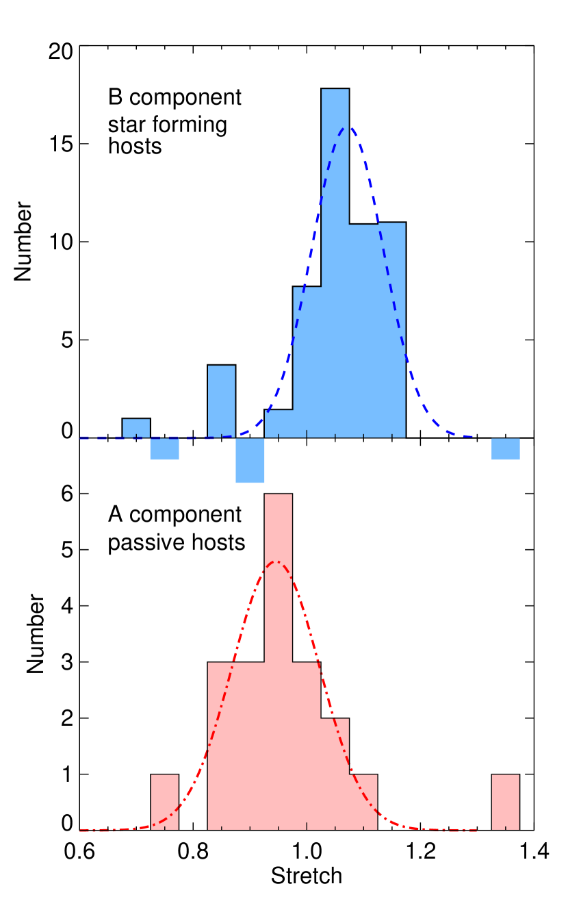
Figure 1.— Stretch distributions of SNe from each component of the two component model. Top: Prompt ($B$-component) SNe Ia. Bottom: Delayed ($A$-component) SNe Ia. The distributions were derived from those in S06, as described in the text. Best-fit Gaussians are shown. The $A$-component Gaussian is centered at $s=0.945$, with $\sigma=0.077$. The $B$-component Gaussian is centered at $1.071$ with $\sigma=0.063$.

The prompt and delayed SN Ia components have different stretch distributions (S06). To determine the stretch of each SN, here we use the SNe from S06, though we fit a new lightcurve template to the data using the SiFTO method (Conley et al., 2007a, b). Because stretches are always defined relative to the $s=1$ template lightcurve, stretch values should only compared within a publication. However, the stretches derived here are approximately 4% larger than those in Astier et al. (2006), largely due to the use of a narrower $s=1$ template.

All SNe from passive galaxies (i.e. those with no measurable star formation rate) were assigned to the $A$ component. Star forming galaxies have SNe Ia from both components, so the $A$ distribution from passive galaxies was scaled by mass and subtracted from the distribution of SNe Ia from star forming galaxies, leaving the $B$ distribution (as in S06). The resulting distributions, and Gaussian fits are shown in Figure 1. Note that to conserve the total number of SNe one should add the SNe subtracted from the $B$ distribution back to the $A$ distribution – this is unnecessary for our purposes because the relative heights of the gaussians are normalized as a function of redshift in the next step.

To estimate the expected stretch evolution with redshift, we take the observed $A$ and $B$ distributions and scale them to the predicted relative values with redshift from Fig. 10 of S06. Increasing cosmic star formation with redshift produces a larger fraction of SNe from the prompt component. Stellar mass as a function of redshift is determined by integrating the star formation history from the earliest times, so the total stellar mass, and the number of SNe from the A component, decreases with increasing redshift. The net result is that in the $A+B$ model the mean stretch increases from 0.98 at $z=0$ to 1.04 at $z=1.5$.

One caveat is that in the $A+B$ model there is no time dependence for the $A$ component. SNe Ia from 10 Gyr old progenitors are just as likely as SNe Ia from 3 Gyr old progenitors. If 10 Gyr-old SNe Ia are actually more rare, the $A+B$ model will overpredict the number of $A$-component SNe at $z=0$, as they result from stars formed during the high star formation rate in the early universe (see discussion in S06). As an alternative to the $A+B$ model we tested the two component SN Ia delay time distribution from Mannucci, Della Valle, & Panagia (2006), which has an exponential decrease in supernova probability from the delayed component with time. The drawback of this model is that the probability distribution is somewhat arbitrary. Also, rather than the 50-50 split between prompt and delayed SNe chosen by Mannucci, Della Valle, & Panagia (2006), here we scale each component by the $A$ and $B$ values measured by S06. This gives similar results to the $A+B$ model, predicting a shift in mean stretch from 0.98 to 1.02 from $z=0-1.5$.

3. Comparison to Observations

In Figure 2 we compare the predicted stretch distributions from the $A+B$ model to the observed stretch distributions in three redshift bins from the low redshift data used by Astier et al. (2006), the SNLS data in S06, and the data of the higher-z supernova search (Riess et al., 2007). All lightcurves have been refit here using the same method. We also tested the data against the modified Mannucci, Della Valle, & Panagia (2006) model, but we did not find it to be a better predictor of SN evolution with redshift (Table 1).

Table 1$\chi^{2}$ and KS test: data and models

	$\chi^{2}$		KS
z	A+B	MM	A+B	MM
0-0.1	0.81	0.63	15%	39%
0.1-0.75	0.64	0.83	30%	28%
0.75-1.5	0.60	0.84	52%	35%

Note. — Cols. 2-3: the $\chi^{2}$ per degree of freedom between the data and the predictions of the A+B and modified Mannucci (MM) models. Cols. 4-5: KS-test probability that the data is drawn from each model. Bins with zero counts were assigned an error of 1.15, possibly underestimating the $\chi^{2}$. The KS test is also imperfect because probabilities were derived for a single Gaussian, not the sum of two Gaussians as used here. In both cases the two model components were fixed by the A and B numbers in S06.

Each survey has different selection effects – the most serious for the current study is Malmquist bias, the tendency to discover only the brightest members of a group near the detection limit of a magnitude-limited survey. To minimize the effect, for each of the high redshift searches we only consider supernovae from a reduced volume so that none of the supernovae used are near the magnitude limit. The SNLS regularly discovers SNe Ia out to $z>1$, but here we use only the subset with $z\leq 0.75$, where Malmquist bias is minimal (Astier et al., 2006). Similarly, we only use Riess et al. (2007) SNe with $z<1.5$, where the authors report their sample is complete (Strolger et al., 2004). Lowering the redshift cuttoff to $z=1.2$ does not change the average stretch for the highest-z sample, but it reduces the sample size from 20 to 13, and thus decreases the significance of the results.

As an additional protection against selection bias, we only consider SNe with $s\geq 0.7$. SNe Ia with $s<0.7$ are both dim and spectoscopically peculiar, like SN 1991bg (Filippenko et al., 1992), and have not yet been detected at $z>0.2$, probably because of a combination of Malmquist bias and spectroscopic selection bias (Howell, 2001; Howell et al., 2005) – as redshift increases, and the angular size of the host galaxy decreases, and it becomes more and more difficult to spectroscopically identify such faint supernovae when blended with their bright, often elliptical, hosts. This cut removes 3 SNe Ia from the low-z sample [other low-z SNe are already removed because we only consider Hubble-flow SNe Ia, with $z>0.015$, to be consistent with Astier et al. (2006)].

In all cases we use only SNe Ia with at least 4 lightcurve points, and at least one detection before 10 rest-frame days after maximum light in the $B$-band, so that stretch is accurately measured.

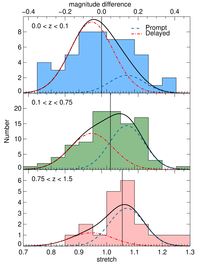
Figure 2.— Actual stretch distributions compared to predictions from the $A+B$ model. In each case the $A+B$ model evaluated at the median redshift of the distribution is shown. Top: SNe Ia from $z=0-0.1$ (median $z=0.026$; N=50). Middle: SNLS SNe Ia from $z=0.1-0.75$ (median $z=0.55$; N=99). Bottom: Riess et al. (2007) SNe Ia from $z=0.75-1.5$ (median $z=1.12$; N=20), with $s$ errors $<0.2$ (requiring $s$ error $\leq 0.1$ reduces the sample to 16 and increases the average stretch from 1.06 to 1.07). The vertical line gives the mean stretch for each distribution. The top axis converts a stretch difference into a magnitude difference using $\alpha=1.5$.

Figure 2 shows that the average observed stretch increases with redshift, from $s=0.98\pm 0.02$ at a median redshift of $z=0.03$, to $s=1.02\pm 0.01$ at $z=0.56$, and $s=1.06\pm 0.02$ at $z=1.12$. Simultaneously the percentage of SNe Ia with $s<0.9$ decreases from 24% to 15% to 1.4%. The KS test gives a 2% probability that the lowest and highest redshift sample are drawn from the same distribution. The predicted distributions from the $A+B$ model are overplotted. The observed trends match the predictions of the empirically-based models — with increasing redshift fewer low-stretch SNe Ia are observed, and the mean SN Ia stretch increases. We find the same result when this analysis is repeated with the SALT (Guy et al., 2005) and SALT2 (Guy et al., 2007) lightcurve fitters. These results are also consistent with the findings of Astier et al. (2006), that the low-z sample had an average stretch 97% that of SNLS SNe.

Astier et al. (2006) estimate distances from SNe Ia using

$$\mu_{B}=m^{*}_{B}-M+\alpha(s-1)-\beta c,$$

where $\mu_{B}$ is the distance modulus, $m^{*}_{B}$ is the peak $B$-band magnitude, $c$ is a color, and $M$, $\alpha$ and $\beta$ are parameters fit by minimizing residuals on the Hubble diagram. Astier et al. (2006) found $\alpha=1.52$, so a drift in average stretch of $0.08\pm 0.026$ from $z=0.03$ to $z=1.12$ results in a 12% drift in average intrinsic SN Ia luminosity over this redshift range.

4. Effect on Cosmological Studies

Evolution in the SN population will not necessarily bias cosmological studies, since SNe are only used in this way after correction for lightcurve shape. However, we can no longer assume that any deficiencies in lightcurve width correction schemes will average out under the assumption the distribution of SNe is similar over all redshifts. If there is a systematic residual between low stretch and high stretch SNe when they are stretch corrected, this could cause a bias in the determination of cosmological parameters as the population evolves.

Figure 3.— Cosmological fits done with the Astier et al. (2006) sample (dashed), and with SNe Ia drawn from the same sample, but using only $s<1$ SNe Ia at $z<0.4$ and $s\geq 1$ SNe Ia at $z\geq 0.4$ (solid). Combining with Baryon Acoustic Oscillation results (Eisenstein et al., 2005) produces the thick lines. The results are consistent at the one sigma level.

To test an extreme case of evolution, we fit the equation of state parameter for dark energy, $w$ and the matter density, $\Omega_{M}$ using the data from Astier et al. (2006), (dashed lines in Fig. 3) and compared it to a fit using the same data, but retaining only $s<1$ SNe Ia at $z<0.4$ and only $s\geq 1$ SNe Ia at $z\geq 0.4$ (solid lines). The strongly evolving subset gives estimates for $w$ and $\Omega_{M}$ consistent with the full set, although the errors are larger because there are fewer SNe in the subset.

One worry with an evolving population is that stretch-magnitude or color-magnitude relations may evolve, i.e. $\alpha$ or $\beta$ derived at one redshift may not be appropriate at another. The values derived here for the strong evolution subset and the full set are consistent, but again a strong test awaits a larger data set.

Measuring changes in $w$ with time will require much stricter control of potential evolutionary effects. Possible biases depend critically on the exact nature of the evolution, the experimental design, the cosmology, and how the time variable component of $w$ is parameterized — e.g. $w\prime$, $w_{1}$, or $w_{a}$ (Weller & Albrecht, 2002; Kim et al., 2004; Linder, 2006). However, a good rule of thumb is that to keep systematic errors significantly below statistical errors for a mission such as SNAP, the corrected magnitudes of SNe Ia should not drift by more than 0.02 mag up to $z=1.7$ (Kim et al., 2004). Unfortunately there are not enough well measured SNe Ia in the literature to determine whether or not stretch correction works to this level of precision. After stretch correction, the rms scatter of SNe Ia around the Hubble line is $\sim 0.2$ mag in the best cases (Guy et al., 2007). Therefore $\sim 100$ SNe Ia are required in each of several stretch or redshift bins to determine whether biases remain at the 0.02 level after correction. Such precise tests will soon be possible by combining data from large surveys underway at low and high redshift.

5. Discussion

We have shown that there is some evolution in the average lightcurve width, and thus intrinsic luminosity of SNe Ia from $z=0$ to $z=1.5$, although significant evolution is found only over a large redshift baseline. This evolution is consistent with our predictions from the $A+B$ model – as star formation increases with redshift, the broader-lightcurve SNe Ia associated with a young stellar population make up an increasingly larger fraction of SNe Ia.

Though we have taken steps to minimize the effects of Malmquist bias, it is possible that residual effects play some role in increasing average stretch with redshift. However, the net effect on cosmology studies is the same no matter the underlying cause. In either case, there is increased pressure on the light curve shape calibration method to correct for the evolution in SN Ia properties with redshift.

Perlmutter et al. (1999) found that SNe Ia still give evidence for an accelerating universe even if SNe Ia are not corrected for stretch. This was possible because the difference in a universe with dark energy and one with $\Omega_{M}=1$ is large — 0.25 magnitudes at $z=0.7$, whereas the population evolution seen here implies that average SN Ia magnitudes should increase by 0.07 mag over the same redshift range. However, discriminating between dark energy models requires much more precise control of SN Ia magnitudes over a larger redshift baseline.

Most theoretical studies addressing possible SN Ia evolution have focused on metallicity. Although theorists have proposed various mechanisms that could conceivably alter the properties of SNe Ia as the average metallicity changes with cosmic time (Höflich, Wheeler, & Thielemann, 1998; Lentz et al., 2000; Domínguez, Höflich, & Straniero, 2001; Timmes, Brown, & Truran, 2003) there is no consensus regarding which effects are important or even the sign of these effects. Observational studies have found no evidence that metallicity affects the properties of SNe Ia (Hamuy et al., 2000; Ivanov, Hamuy, & Pinto, 2000; Gallagher et al., 2005; Ellis et al., 2007). Instead, it is more likely that age differences between the two populations (and thus almost certainly the mass of the secondary star) play a role in the evolution of the observed stretch distribution with redshift (Howell, 2001).

Prompt SNe Ia are thought to be brighter because they produce more ⁵⁶Ni. If the Chandrasekhar-mass model describes most SNe Ia, they must then produce less intermediate mass elements, assuming that the amount of unburned material is negligible in normal SNe Ia. We therefore predict that high redshift SNe Ia will have less Ca and Si. This is confirmed by the most intensive study of high redshift SN Ia spectra (Ellis et al., 2007).

One concern raised by these findings is that pathological SNe Ia such as SN 2001ay (Howell & Nugent, 2004), SN 2002cx (Li et al., 2003), SN 2002ic (Hamuy et al., 2003), and SNLS-03D3bb (Howell et al., 2006), which do not obey typical lightcurve shape correction schemes, are associated with star formation. Since star formation density increases by a factor of ten from $z=0$ to $z=1.5$ (Hopkins & Beacom, 2006), at high redshift these pathological supernovae will be an order of magnitude more common. Thus the conventional wisdom that all high redshift supernovae will have counterparts at low redshift (Branch et al., 2001) only holds if sample sizes are much larger than those currently used for cosmology. Only 20 SNe Ia have published lightcurves at $z>1$ (Riess et al., 2007; Astier et al., 2006), and only $\sim$50 SNe Ia at $z<0.1$ have sufficient data to be cosmologically useful. Fortunately, thus far it has been possible to identify these outliers so that they do not affect cosmological analyses, but future studies requiring increased precision must be vigilant of the effects of an evolving SN Ia population.

References

- Astier et al. (2006) Astier, P. et al. 2006, A&A, 447, 31
- Branch et al. (2001) Branch, D., Perlmutter, S., Baron, E., & Nugent, P. 2001, ArXiv Astrophysics e-prints
- Conley et al. (2007a) Conley, A., Carlberg, R. G., Guy, J., Howell, D. A., Jha, S., Riess, A. G., & Sullivan, M. 2007a, ArXiv e-prints, 705
- Conley et al. (2007b) Conley, A. 2007b, in preparation
- Domínguez, Höflich, & Straniero (2001) Domínguez, I., Höflich, P., & Straniero, O. 2001, ApJ, 557, 279
- Eisenstein et al. (2005) Eisenstein, D. J. et al. 2005, ApJ, 633, 560
- Ellis et al. (2007) Ellis, R. 2007, in preparation
- Filippenko et al. (1992) Filippenko, A. V. et al. 1992, AJ, 104, 1543
- Gallagher et al. (2005) Gallagher, J. S., Garnavich, P. M., Berlind, P., Challis, P., Jha, S., & Kirshner, R. P. 2005, ApJ, 634, 210
- Guy et al. (2007) Guy, J. et al. 2007, A&A, 466, 11
- Guy et al. (2005) Guy, J., Astier, P., Nobili, S., Regnault, N., & Pain, R. 2005, A&A, 443, 781
- Hamuy et al. (1995) Hamuy, M., Phillips, M. M., Maza, J., Suntzeff, N. B., Schommer, R. A., & Aviles, R. 1995, AJ, 109, 1
- Hamuy et al. (2003) Hamuy, M. et al. 2003, Nature, 424, 651
- Hamuy et al. (2000) Hamuy, M., Trager, S. C., Pinto, P. A., Phillips, M. M., Schommer, R. A., Ivanov, V., & Suntzeff, N. B. 2000, AJ, 120, 1479
- Höflich, Wheeler, & Thielemann (1998) Höflich, P., Wheeler, J. C., & Thielemann, F. K. 1998, ApJ, 495, 617
- Hopkins & Beacom (2006) Hopkins, A. M. & Beacom, J. F. 2006, ApJ, 651, 142
- Howell (2001) Howell, D. A. 2001, ApJ, 554, L193
- Howell & Nugent (2004) Howell, D. A. & Nugent, P. 2004, in Cosmic Explosions in Three Dimensions, 151
- Howell et al. (2006) Howell, D. A. et al. 2006, Nature, 443, 308
- Howell et al. (2005) Howell, D. A. et al. 2005, ApJ, 634, 1190
- Ivanov, Hamuy, & Pinto (2000) Ivanov, V. D., Hamuy, M., & Pinto, P. A. 2000, ApJ, 542, 588
- Jha, Riess, & Kirshner (2007) Jha, S., Riess, A. G., & Kirshner, R. P. 2007, ApJ, 659, 122
- Kim et al. (2004) Kim, A. G., Linder, E. V., Miquel, R., & Mostek, N. 2004, MNRAS, 347, 909
- Lentz et al. (2000) Lentz, E. J., Baron, E., Branch, D., Hauschildt, P. H., & Nugent, P. E. 2000, ApJ, 530, 966
- Li et al. (2003) Li, W. et al. 2003, PASP, 115, 453
- Linder (2006) Linder, E. V. 2006, Astroparticle Physics, 26, 102
- Mannucci, Della Valle, & Panagia (2006) Mannucci, F., Della Valle, M., & Panagia, N. 2006, MNRAS, 370, 773
- Mannucci et al. (2005) Mannucci, F., della Valle, M., Panagia, N., Cappellaro, E., Cresci, G., Maiolino, R., Petrosian, A., & Turatto, M. 2005, A&A, 433, 807
- Perlmutter et al. (1999) Perlmutter, S. et al. 1999, ApJ, 517, 565
- Perlmutter et al. (1997) Perlmutter, S. et al. 1997, ApJ, 483, 565
- Phillips (1993) Phillips, M. M. 1993, ApJ, 413, L105
- Prieto, Rest, & Suntzeff (2006) Prieto, J. L., Rest, A., & Suntzeff, N. B. 2006, ApJ, 647, 501
- Riess et al. (1998) Riess, A. G. et al. 1998, AJ, 116, 1009
- Riess, Press, & Kirshner (1996) Riess, A. G., Press, W. H., & Kirshner, R. P. 1996, ApJ, 473, 88
- Riess et al. (2007) Riess, A. G. et al. 2007, ApJ, 659, 98