Paleontology of Galaxies: Recovering the Star Formation & Chemical Enrichment Histories from Galaxy Spectra

Resumen

Recent advances in stellar population modelling and avalanches of data from mega-surveys have revived the interest in techniques to extract information about galaxy evolution from integrated spectra. This contribution provides an informal and (hopefully) pedagogical, but inevitably biased and incomplete introduction to this field. Emphasis is given to the several choices one has to make in the process of modelling galaxy spectra.

INVITED PAPER

(1) Depto. de Física, Universidade Federal de Santa Catarina (Brasil)

Resumen.   Los recientes avances en modelos de poblaciones estelares y la avalancha de datos de mega-surveys han revivido el interés en técnicas para extraer información acerca de la evolución de galaxias a partir de espectros integrados. Esta contribución presenta una introducción informal y pedagógica, pero inevitablemente sesgada e incompleta, a este tema, con énfasis en las varias elecciones que uno tiene que hacer en el proceso de modelar espectros de galaxias.

1. Introduction

The Wikipedia entry for “paleontology” states that it “is the study of the history and development of life on Earth, including that of ancient plants and animals, based on the fossil record”. Much of astronomical research shares this same general goal: To study how things form and evolve, be they planets, stars, galaxies or the universe as a whole.

A great deal of current work is focused on finding and characterizing galaxies as far as possible. Since far in space = far in time, observations at different redshifts ($z$) sample different stages in the history of galaxies. Studying how galaxy properties (or relations between properties) change with $z$ gives us important clues on evolutionary processes. The evolution of the mass-metallicity relation, for instance, has now been extended to intermediate and high $z$’s (e.g., Savaglio et al. 2005; Shapley et al. 2005), and comparison with its local universe counterpart reveals systematic offsets which ultimately reflect the history of metal enrichment along cosmic time. Similarly, the (Tully-Fisher) relation between luminosity and rotation speed has been mapped at different lookback times in search of evolutionary effects (Aragón-Salamanca 2006). These are just two examples of the thriving times of current observational cosmology.

Paleontologists would have a much easier life if they had a “time-machine” as nice as the universe! No more digging on dirty swamps or hot deserts, no more trying to figure what a dinosaur looked like from a couple of broken bones. Just find a few Earth like places whose clocks mark different evolutionary times, and see how things were and how evolution proceeded over the years.

Though promising, the high-$z$ work does not (yet) compete with local universe studies in terms of data quality and specially quantity. Limits on data quality, say low $S/N$ spectra, propagate to limits in the amount of information that can be extracted about galaxian histories. Quantity is equally important. Whereas just a few years ago we would be happy with 2 or 3 digits samples, mega-surveys like the 2dF and SDSS have taught us what a difference $N$ makes! Galaxy evolution is surely not a simple 1 or 2 parameter problem. A helpful strategy to tackle complex multi-dimensional problems is to break a sample in narrow ranges of physical or observational properties (say, mass and environment and color), which requires very large samples. Kauffmann et al. (2003), Brinchmann et al. (2004), Clemens et al. (2006), Mateus et al. (2006) and Muriel’s paper in this same volume are examples of studies which benefited from $N\sim 10^{5\pm 1}$ statistics.

But how can we dig the history of galaxies from cosmologically shallow surveys, which barely reach a tenth of a galaxy’s life?

2. Fossil methods

This is where the analogy with paleontology fits in. Faced with fossils from different epochs, a paleontologist tries to figure, with the help of ancillary data and/or theories, how things unfolded as time passed. A galaxy spectrum can be seen as a fossil record of its history. The old, low mass stars which shine today in elliptical galaxies are just the long-lived relics of a hectic past, where stars formed at high rates and massive stars dominated the scene. The gas and just-born stars which make up today’s HII regions in spirals coexist with the low mass survivors of previous generations, whose long-gone massive stars contributed to the metals now shining under the ionizing photons of younger generations.

The age and metal content of young and old stars leave their fingerprints as colors and absorption lines. Hence, a galaxy’s spectrum contains information from all its stellar generations. This is good news. The bad news is that unscrambling this crazy mixture of photons coming from $\sim$ the same space but reflecting different cosmic times is no easy task. The difficulties, both mathematical and astrophysical, are best appreciated with some basic formalism.

The most general strategy to tackle this puzzle is to consider a galaxy as a sum of simple stellar populations (SSP), each with its age ($t_{j}$) and metallicity ($Z_{j}$), such that a galaxy spectrum can be written as:

$$L_{\lambda}^{gal}(\vec{x})=\sum_{j=1}^{N_{\star}}L^{SSP}_{\lambda,j}=L_{\lambda_{0}}^{gal}\sum_{j=1}^{N_{\star}}x_{j}l^{SSP}_{\lambda,j}$$ (1)

where $l^{SSP}_{\lambda,j}(t_{j},Z_{j})$ is the spectrum of the $j^{th}$ population normalized at a reference wavelength $\lambda_{0}$, and $\vec{x}$ is the so called population vector, which says what fraction of the galaxy light at $\lambda_{0}$ comes from the $j^{th}$ population, i.e., from stars of age $t_{j}$ and metallicity $Z_{j}$. Equivalently, one may express the problem in terms of mass fractions, which relate to $\vec{x}$ via the $M/L_{\lambda_{0}}$ of each population. One then compares this model with an observed spectrum $O^{gal}_{\lambda}$ (or indices derived from it) and seeks the $\vec{x}$ which minimizes residuals:

$$\chi^{2}=\sum_{\lambda}[O^{gal}_{\lambda}-L^{gal}_{\lambda}(\vec{x})]^{2}w_{\lambda}^{2}$$ (2)

where $w_{\lambda}$ is the weight attributed to pixel $\lambda$. This equation is incomplete in at least two senses. First, it lacks a term to account for the Doppler shifts caused by the way stars move around in a galaxy, smoothing absorption lines on scales of order 100 km s^-1. This effect is easily modeled convolving equation 1 with a kinematical filter, so let’s pretend this has been done. Secondly, extinction terms, which affect galaxy spectra on a much larger $\lambda$-scale, are missing. Extinction can and must be modelled, and the simplest thing to do is to model it as a homogeneous foreground dust screen, multiplying 1 by $10^{-0{,}4(A_{\lambda}-A_{\lambda_{0}})}$ and choosing some $A_{\lambda}/A_{\lambda_{0}}$ reddening curve. Though this strategy gives useful results, it entails a blatantly simplistic representation of real galaxies, where different populations are affected differently by dust. Accounting for this in a consistent and robust way is perhaps the most serious challenge for current population synthesis methods. In the absence of a solid technique to deal with this difficulty, we are forced to adopt the traditional method of forgetting the problem and adopting the screen model until further notice.

Clearly, it is $\vec{x}$ we are after, as it encodes the distribution of stellar ages and metallicities, and hence the whole star formation history (SFH) of a galaxy. To get there, we need to specify several things.

2.1. The basis

What should we use for $l^{SSP}_{\lambda,j}$? In other words, which the basis in which we are going to decompose our model for $L_{\lambda}^{gal}$? The superscript “SSP” already tells what my favorite answer is. Thinking of a galaxy spectrum in terms of a sum of SSPs is the simplest reasonable thing one can think of. One then needs to decide where will the basis spectra $l^{SSP}_{\lambda,j}$ ($j=1\ldots N_{\star}$) be drawn from.

One approach, founded by Bica & Alloin in the 80’s, is to use observed star cluster spectra. This strategy has proven quite successful, and is still being actively pursued, as illustrated by the work of Ahumada in this same volume. An advantage of using observed clusters is that one mimics Mother Nature as best as possible, without having to resort to assumptions about initial mass function, stellar evolution and stellar spectra. A disadvantage is that observed clusters do not span the whole $t$-$Z$ space homogeneously (and curing this deficiency is precisely one of the motivations of Ahumada’s work). Bica (1988) was the first to apply this technique to infer galaxian SFHs.

Alternatively, one may use models for $l^{SSP}_{\lambda,j}$. The modelling of SSP spectra has evolved so much that nowadays one can fit observed cluster spectra close to perfection. Despite the larger load on assumptions, theoretical $l^{SSP}_{\lambda}$’s can replace observed ones with the advantage of a wider coverage of the $t$-$Z$ plane and spectral range. Up to the publication of medium spectral resolution ($\lambda/\Delta\lambda\sim 2000$) models by Bruzual & Charlot (2003, BC03), soon followed by similar work by Le Borgne et al. (2004), Gonzalez-Delgado et al. (2005) and others, this approach enjoyed limited use. Since then, however, it has boomed.

These are not the only alternatives. Instead of a summation of SSPs one can model the SFH of galaxies in more continuous terms, adjusting equation 1 to an integral and so on. An exponentially declining star-formation rate function, for instance, is a quite popular recipe. Instantaneous or finite duration bursts may be superimposed to this continuous regime, and in fact any other ad hoc or physically motivated parameterization may be implemented. As long as one allows for many SSPs in 1 (i.e., $N_{\star}\gg 1$), the discrete SSP-based approach encompasses more continuous descriptions of galaxy histories. Given the many things which can spur star formation throughout a galaxy’s life, a non-parametric approach sounds more advisable.

2.2. Observables: Indices $\times$ Full Spectrum

Having decided what spectral basis to use, you must specify your observables, ie, what it is exactly that you will try to fit. Eq. 1 is written to model the pixel-by-pixel spectrum of a galaxy, clearly the most complete approach possible. Historically, however, astronomers have most often chosen to model not the full $L^{gal}_{\lambda}$, but spectral indices such as absorption line equivalent widths and/or colors. Indices can be seen as a compressed, but highly informative, representation of the whole spectrum.

A particularly influential set of absorption line indices has been defined by the Lick Observatory group on the basis of low resolution spectra of a library of stars. These so called “Lick indices” have been at the center stage of research on old stellar populations, particularly in elliptical galaxies, for over 20 years (see Rose 2007 for a recent review). The sensitivity of these indices to fundamental stellar parameters ($T_{eff}$, $\log g$ and $Z$) was calibrated and models were constructed which map their behavior in terms of the $t$ and $Z$ of SSPs. Another important set of indices was defined by Bica & Alloin (1986) on the basis of star-cluster data of resolution similar to the Lick library. Star clusters of all ages were included, which allowed Bica (1988) to apply his synthesis method to late type galaxies as well as ellipticals. (Again, see Ahumada’s contribution elsewhere in this volume for updates on this line of work.)

In the past few years, the publication of medium and high resolution, wide $\lambda$-coverage libraries of stars across the HR diagram and the implementation of such libraries into evolutionary synthesis codes allowed the first attempts to model galaxy spectra on a pixel-by-pixel basis. This represented a “phase-transition” in the field, a transition which is quickly being consolidated with the ongoing release of new and more complete libraries. While indices will still be around for years to come, there is a very strong push towards full spectral fits.

Before fitting a spectrum, you have to decide whether the flux calibrations of your data and the basis spectra are reliable. If they are not, or if for whatever reason (say, you would like to dribble extinction issues) you do not care about the continuum, you can still fit a rectified spectrum.

2.3. Method

Once you’ve defined a parameter space (§2.1.) and your favorite observables (§2.2.), it’s time to figure a way from going from one to the other, ie, to estimate your chosen parameters given your data. So many methods to do this journey have been proposed that I will not dare to even briefly review it (see Cid Fernandes 2007 for a review). Suffice it to say that this is not an easy task. If your parameter space is of low dimensionality, life may be easier, since you have already simplified your problem beforehand with your own preconceptions (“priors”, in the Bayesian lingo). For instance, you may want to model a whole galaxy as a single population, in which case your task is to find the best $t$ and $Z$ (and perhaps $\alpha$/Fe, if your basis allow for it), and relatively straight-forward fitting techniques can be used. This would be essentially equation 1 with $N_{\star}=1$. Ellipticals are often modeled in this fashion. More complex/realistic models are obviously desirable, particularly for spirals, where the SFH is surely not even remotely like a single burst. The larger the parameter space (i.e., larger $N_{\star}$), the harder it is to explore it, and the more degenerate the problem becomes.

Degeneracies are a recurrent theme in this business, and a source of considerable confusion. Methods based on indices often try to recover more populations than observables, ie., $N_{\star}>N_{\rm indices}$, and people doing this have sometimes been wrongly accused of being able to fit anything they want. Pelat (1998), in a very elegant paper, shows that this is not true at all. If your basis is not right and/or your data have errors, what could in principle be a problem with infinite exact solutions may turn out to have none! And even if there are infinite solutions, it is possible to determine the subspace of the parameter space which maps onto the data space. This does not eliminate degeneracies, but it tells you what the acceptable solutions are, and this is valuable information. Besides algebraic issues, astrophysical effects also conspire against unique solutions. The most (in)famous such degeneracy is the one between $t$ and $Z$. Red and strong lined galaxies may be modeled as having old ages or large metallicities, such that old, metal poor $\vec{x}$ components in equation 1 can be swapped by younger and higher $Z$ components without much change in $L_{\lambda}^{gal}$, and vice-versa. In general, components with similar $l^{SSP}_{\lambda,j}$ spectra are hard to be distinguished. For instance, it is hopeless to try to distinguish 4 from 5 Gyr old populations with spectra of realistic S/N. Current estimates of the age-resolution achievable with inversion methods place it in the $\Delta\log t\sim 0{,}5$–1 dex range.

Degeneracies are thus an inescapable fact-of-life in population synthesis, and one must learn to live with them! The simpler strategy to deal with this is to downsize your expectations and work with a relatively coarse description of SFHs.

This can be done in a number of ways. For instance, you may start with the number of components which you believe you are able to recover when fitting realistic galaxy spectra, as done in the MOPED code (e.g., Panter et al. 2003). STECMAP (Ocvirk et al. 2006) achieves this same general goal applying regularization techniques which impose that the derived SFH be a smooth function of time. My own code, STARLIGHT (Cid Fernandes et al. 2005), uses a ridiculously large $N_{\star}$ (of order 100), but when it comes to describe SFHs a reduced version of $\vec{x}$ is used, grouping components of similar properties. Compression of the population vector may thus be carried out a priori, on the fly, or a posteriori.

There are numerous technical and astrophysical differences between currently existing methods to go from the data to the parameters. Some account for extinction, some don’t. Some include kinematics, others don’t. Some impose simple $Z$-$t$ relations, some use a fixed $Z$ and others treat $Z$ and $t$ independently. Some model indices, others the full spectrum. Some compute combinations of basis elements on the fly, others compare the data to a large library of precomputed models. Last but not least, there are also differences in the spectral basis.

Given this bewildering diversity, I would not be surprised to see a proportionately large diversity in the results. To my surprise, a test carried out at IAU Symposium 241 showed an amazing degree of convergence among all methods. Either we all got it right, or we are all doing the same mistakes! Let us suppose we are on the right track and show some results.

3. Results: A brief tour of spectral fits with STARLIGHT

After this necessarily simplified introduction, this section illustrates what kind of results can be achieved with state-of-the-art population synthesis methods. All results below were obtained with the code STARLIGHT described in Cid Fernandes et al. (2004, 2005) and Mateus et al. (2006). STARLIGHT has been successfully applied to spectra of normal galaxies, Seyfert nuclei, LINERs, Transition Objects, quasars, luminous infrared galaxies, and others, with data qualities spanning the full horrible–marvelous range. Let’s see what we obtain.

Figure 1.: Examples of STARLIGHT fits to an AGN (left) and a star-forming galaxy (right) from the SDSS. The top panels panels show the observed (black) and model (red) spectra, while the bottom ones show the residuals, with emission lines and bad pixels are marked in green Green. The smaller panels show the derived age distribution in light (top) and mass (bottom) fractions.

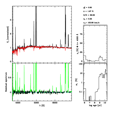
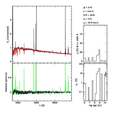
Fig. 1 shows fits to 2 of the nearly 600000 SDSS galaxies which have already been modeled with STARLIGHT. The fits were carried out with a basis of SSPs spanning 25 ages and 6 metallicities ($N_{\star}=150$!) from BC03. The left panels plot the observed, model and difference spectra, while the right panels show the inferred light and mass population vectors without any compression apart from the marginalization over $Z$. Estimates of the SFH and chemical enrichment histories, starlight extinction, velocity dispersion and stellar masses have been obtained for all galaxies. Emission lines measurements, for which accurate subtraction of the stellar spectrum is critical, have also been measured, yielding estimates of nebular metallicity, H$\alpha$/H$\beta$-extinction, line widths and etc.

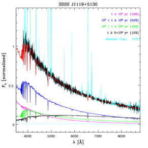
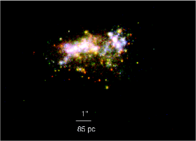
Fig. 2 shows a STARLIGHT fit to the SDSS spectrum of an Ultra Compact Blue Dwarf Galaxy (Corbin et al. 2006). 25 ages but only $Z_{\odot}/50$ SSPs were included in the fits of these SMC-like galaxies, which, despite looking extremely young, have most of their stellar mass locked up in old, $\sim 10$ Gyr stars. As in IZw18, the ongoing star formation performs a pretty good “plastic surgery” in these systems, but not effective enough to hide its true age from the synthesis. The plot groups the 25 components of $\vec{x}$ onto just 4 relevant age bins, illustrating our a posteriori compression approach.

Figure 2.: HST color image and STARLIGHT fit to the spectrum of SDSS J1119+5130. The observed and model spectra are shown in black and red, respectively, Emission lines and bad pixels (turquoise) were masked in the fits. The bottom spectra are sums of the constituent SSP spectra in four age bins, whose contributions to the observed flux at 4020 Å are shown in parentheses. See Corbin et al. (2006) for details.

The astute reader may be wondering whether the success stories told by Figs. 1 and 2 are just due to the fact that we are fitting relatively noisy data. While it is true that fitting good data is always harder, Fig. 3 shows that STARLIGHT is also capable of dealing with $S/N\sim 100$ spectra. (This exquisite spectrum was obtained by Paula Coelho and Claudia Mendes de Oliveira.) Data and model can hardly be told apart!

Figure 3.: Section of a high $S/N$ Gemini spectrum modeled with STARLIGHT. Observed and model spectra are shown in black (solid) and red (dotted) respectively (Coelho et al. 2007, in prep.).

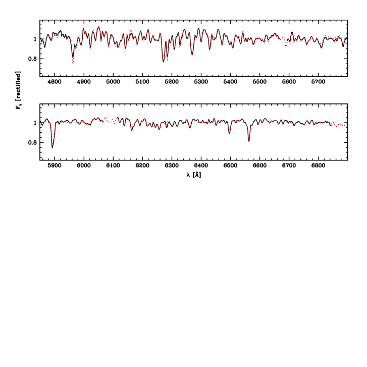
The message from this quick tour is that one can nowadays model galaxy spectra on a pixel-by-pixel basis with an unprecedented degree of success. Though all examples are based on STARLIGHT, I am sure that MOPED, STECMAP, and other “competing” codes would perform equally well, which lends credibility to spectral fits.

4. Checks, caveats and final words

By themselves, spectral fits may look good and be very helpful to derive pure-emission spectra. Their main utility, however, is to derive the SFH of galaxies. Many interesting results have emerged in recent years, both using just the first moments of the $t$ and $Z$ distributions and the full SFHs. Instead of reviewing these astrophysical results (see Cid Fernandes 2007 and references therein), I prefer to end this contribution illustrating a couple of the many sanity checks which we have carried out, and an illustration of how things which go wrong can also teach us important lessons.

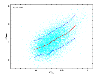
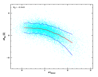
As already mentioned, naive modeling of dust effects is perhaps the major caveat in spectral fits. To check whether the fits are producing at least sensible results, we have correlated the derived values of $A_{V}$ with those derived from the H$\alpha$/H$\beta$ ratio. Fig. 4 shows that these two independently quantities correlate very strongly. Not only that, we find that stars suffer about half the extinction that affects the gas, in amazing agreement with detailed studies of nearby star-forming galaxies (Calzetti et al. 1994). Fig. 4 shows a further test of the consistency of the synthesis results. We correlate the nebular extinction, $A_{V}(H\alpha/H\beta)$, with the strength of the residual NaD absorption doublet, which traces the cold ISM component. The gratifyingly evident relation between these two independently derived quantities gives us confidence that our results are meaningful, despite the over-simplified dust geometry adopted. Cid Fernandes et al. (2005) and Asari et al. (2007, in prep.) present further sanity checks.

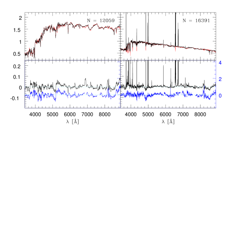
Having spent so many lines emphasizing how great spectral fits are, it is fitting to warn you that they are not perfect. Fig. 5 illustrates this. What is shown there are the stacked results of fits for many thousands of high $S/N$ elliptical (left) and late-type, star-forming galaxies (right) from the SDSS. The top panels show the mean observed and model spectra. Seen in their natural scales, the fits look perfect. However, zooming on the the mean residual spectra (bottom panels) reveals several systematically miss-fit spectral features.

In elliptical galaxies, features associated to $\alpha$ elements, like the Mg, CN and Na bands, are all under-fitted. This is not surprising, given that the library used by BC03 is fundamentally based on solar neighborhood stars, whose chemical abundance pattern are known to differ from stars in early type systems. In star-forming galaxies, selected on the basis of emission line diagnostic-diagrams, the most obvious problem is a shallow but broad “absorption” band around H$\beta$, which appears whenever stars of $\sim 100$ Myr are present in large proportions. Unlike the problems for $\alpha$-related bands in ellipticals, there is no straightforward physical explanation nor element identification for this trough. We suspect that this is not an absorption band at all, but a side-effect of flux calibrations issues in STELIB, maybe associated to the fact that stars with wide H$\beta$ absorption were used as flux standards. In any case, these miss-fits illustrate how the analysis of galaxy spectra can provide useful feedback to those constructing stellar and SSP spectral libraries. It will be important to repeat this practical-tests with the new libraries to evaluate whether they do bring the expected improvements.

Figure 4.: Left: Nebular versus stellar extinction for high $S/N$ star-forming galaxies in the SDSS. Right: Equivalent width of the NaD $\lambda\lambda$5890,5896 doublet, measured from the residual spectrum, against the nebular extinction derived from H$\alpha$/H$\beta$ for star-forming galaxies. Lines mark the 5, 50 and 95 % percentiles.

Figure 5.: Top: Mean observed spectra (black) and their respective models (red) for thousands of high $S/N$ elliptical (left) and star-forming (right) SDSS galaxies, all normalized at 4020 Å. Bottom: Zoom of the Observed $-$ Model (black) and (Observed $-$ Model) / Error (blue) residual spectra.

To close, I hope these pages have given you an idea of the several choices one has to make when modelling galaxy spectra, and how this technique to perform “paleontological” studies of galaxies has matured substantially in the past few years due to a combination of advances in theoretical ingredients, mathematical methods and abundance of data. Further progresses in these 3 fronts are expected in the very near future. Clearly, we will have busy and exciting times ahead.

References

Aragón-Salamanca, A. 2006, IAU Symp. 235, in press (astro-ph/0610587)

Bica, E. & Alloin, D 1986, A&AS, 66, 171

Bica, E. 1988, A&A, 195, 76

Brinchmann, J., Charlot, S., White, S. D. M., Tremonti, C., Kauffmann, G., Heckman, T & Brinkmann, J. 2004, MNRAS, 351, 1151

Bruzual, G. & Charlot, S. 2003, MNRAS, 344, 1000

Calzetti, D., Kinney, A. & Storchi-Bergmann, T. 1994, ApJ, 429, 582

Cid Fernandes, R. 2007, IAU Symp. 241, in press.

Cid Fernandes, R., Gu, Q., Melnick, J., Terlevich, E., Terlevich, R., Kunth, D., Rodrigues Lacerda, R. & Joguet, B. 2004, MNRAS, 355, 273

Cid Fernandes, R., Mateus, A., Sodré, L., Stasińska, G. & Gomes, J. M. 2005, MNRAS, 348, 363.

Clemens, M., Bressan, A., Nikolic, B., Alexander, P., Annibali, F. & Rampazzo, R. 2006, MNRAS, 370, 702

Corbin, M., Vacca, W., Cid Fernandes, R., Hibbard, J., Somerville, R. & Windhorst, R. 2006, ApJ, 651, 861

Gonzalez Delgado, R., Cerviño, M., Martins, L. P., Leitherer, C. & Hauschildt, P. H. 2005, MNRAS, 357, 945

Kauffmann G., et al. 2003, MNRAS, 346, 1055

Le Borgne, D., Rocca-Volmerange, B., Prugniel, P., Lançon, A., Fioc, M. & Soubiran, C. 2004, A&A, 425, 881

Mateus, A., Sodré, L., Cid Fernandes, R., Stasińska, G., Schoenell, W. & Gomes, J. M. 2006, MNRAS, 370, 721

Ocvirk, P., Pichon, C., Lançon, A. & Thiébaut, E. 2006, MNRAS, 365, 74

Panter, B., Heavens, A. F. & Jimenez, R. 2003, MNRAS, 343, 1145

Pelat, D. 1998, MNRAS, 299, 877

Rose, J. 2007, IAU Symp. 241, in press.

Savaglio S., et al. 2005, ApJ, 635, 260

Shapley, A. E., Coil, A. L., Ma, Chung-Pei, Bundy, K. 2005, ApJ, 635, 1006