Ly-$\alpha$ forest: efficient unbiased estimation of
second-order properties with missing data

Abstract

Context. One important step in the statistical analysis of the Ly-$\alpha$ forest data is the study of their second order properties. Usually, this is accomplished by means of the two-point correlation function or, alternatively, the $K$-function. In the computation of these functions it is necessary to take into account the presence of strong metal line complexes and strong Ly-$\alpha$ lines that can hidden part of the Ly-$\alpha$ forest and represent a non negligible source of bias.

Aims. In this work, we show quantitatively what are the effects of the gaps introduced in the spectrum by the strong lines if they are not properly accounted for in the computation of the correlation properties. We propose a geometric method which is able to solve this problem and is computationally more efficient than the Monte Carlo (MC) technique that is typically adopted in Cosmology studies. The method is implemented in two different algorithms. The first one permits to obtain exact results, whereas the second one provides approximated results but is computationally very efficient. The proposed approach can be easily extended to deal with the case of two or more lists of lines that have to be analyzed at the same time.

Methods. Numerical experiments are presented that illustrate the consequences to neglect the effects due to the strong lines and the excellent performances of the proposed approach.

Results. The proposed method is able to remarkably improve the estimates of both the two-point correlation function and the $K$-function.

1 Introduction

The study of the absorption lines observed in the optical spectra of high redshift quasars has greatly evolved in the last decade thanks mainly to the advent of the new class of 10m-telescopes coupled with high resolution, high performance spectrographs and to the improved comprehension of the physical nature of the absorbers.

The lines forming the so called “Ly-$\alpha$ forest” observed blue ward of the Ly-$\alpha$ emission of the quasar are due to the Ly-$\alpha$ transition in neutral hydrogen distributed along the line of sight. They originate in the fluctuations of the intermediate and low density intergalactic medium (IGM), arising naturally in the hierarchical process of structure formation (e.g., Cen et al. 1994; Zhang et al. 1995; Hernquist et al. 1996; Miralda-Escudé et al. 1996; Bi & Davidsen 1997; Davé et al. 1997; Zhang et al. 1997; Theuns, Leonard & Efstathiou 1998; Machacek et al. 2000). Thus, the Ly-$\alpha$ forest provides a unique and powerful tool to study the distribution/evolution of baryonic matter and the physical status of the IGM over a wide redshift interval.

In analogy with the study of galaxies, the two-point correlation function has been classically used to study the distribution of the Ly-$\alpha$ lines (e.g. Sargent et al. 1980). However, the Ly-$\alpha$ distribution is contaminated in the observed spectra by metal transitions associated with galactic haloes pierced by the line of sight. The stronger metal lines can extend for several angstrom covering weaker Ly-$\alpha$ lines and causing a bias in their distribution. The same is true for strong Ly-$\alpha$ absorptions, in particular, Lyman limit and damped Ly-$\alpha$ systems. On the other hand, the distribution at small scales is biased by the intrinsic width of the lines ($\sim 25-30$ km s^-1).

Observers have become more and more aware of those problems in particular for high resolution spectra and at large redshifts where the crowding of the lines increases ($dn/dz\propto(1+z)^{2.5}$, e.g., Kim et al. 2002). In the most recent papers based on high resolution quasar spectra (e.g., Lu et al. 1996; Cristiani et al. 1997; Kim et al. 2001) the strong Ly-$\alpha$ lines are eliminated from the computation of the two-point correlation function and the lines closer than a minimum velocity separation are merged. In order to correct for edge effects and presence of the metal gaps in the line distribution, the observed distribution of line pairs is compared with Monte Carlo (MC) simulations of lines which are randomly distributed in the observed redshift interval other than the cosmological increase with redshift. The same gaps due to the cut-out absorptions are reported also on the simulated spectra and the minimum separation between two lines is preserved. The simulated process is approximately of Poisson type over small redshift separations (see Sargent et al. 1980).

A further approximation is introduced in this method because it is not the redshift split but the velocity split distribution that is considered, where the separation $\Delta v_{ij}$ between two absorption lines of redshifts $z_{i}$ and $z_{j}$ is given by the non linear formula $\Delta v_{ij}=c|(z_{i}-z_{j})|/[1+(z_{i}+z_{j})/2]$. Since, if $\Delta v_{13}>\Delta v_{12},\Delta v_{23}$, it is $\Delta v_{13}\neq\Delta v_{12}+\Delta v_{23}$, the quantities $\Delta v_{ij}$ do not represent Euclidean distances. Hence, from the quantities $\{\Delta v_{i,j}\}_{i,j=1}^{N}$ it is not even possible to construct the one-dimensional point process corresponding to the sequence of the velocities $v_{1},v_{2},\ldots,v_{N}$. The use of velocities at the place of comoving separations was suggested mainly by the unknown ratio between peculiar velocity and Hubble flow contributions to the measured Ly-$\alpha$ line redshifts. There is now evidence that peculiar velocities are negligible for those absorbers (e.g., Rauch et al. 2005; D’Odorico et al. 2006), which makes it preferable to use comoving distances to compute the two-point correlation function.

The computation of a comoving distance corresponding to a given $z$ requires the evaluation of an integral that in general is not available in closed form. Hence, a numerical approach has to be adopted. This can make the MC methods very time consuming. For this reason, in this paper we present a geometric method to compute the two-point correlation that does not require the generation of auxiliary random samples and therefore is much more efficient.

In Sec. 2 the computation of the two-point correlation function and of the $K$-function is considered when only edge effects are present. In Sec. 3 and Appendices A-D the arguments are generalized to deal with the case of gaps in the data sequence and two algorithms are proposed. Two experimental data sets are analyzed in Sec. 4. Finally, conclusions are presented in Sec. 6.

Throughout this paper we will adopt for the cosmological parameters: $\Omega_{0\rm{m}}=0.26,\ \Omega_{0\Lambda}=0.74$, and $H_{0}=73$ km s^-1 Mpc^-1.

2 Estimation of $K(r)$ and $\xi(r)$ in presence of edge effects

A one-dimensional spatial point process $X$ is any stochastic mechanism that generates a countable set of events $\@vec{x}=\{x_{i}\}_{i=1}^{n}$ on the real axis $\mathbb{R}$. It is called stationary if the distribution of $X$ is invariant under translations, that is, the distribution of $X+s$ is the same as that of $X$ for any $s\in\mathbb{R}$. Usually, stationary point processes are described by their first-order and second-order characteristics. The first-order characteristic, say $\lambda$, equals the mean number of points per unit of length and is often called intensity. The second-order characteristics are represented by the two-point correlation function $\xi(r)$ and the pair correlation function $g(r)$ that satisfy

$$g(r)=1+\xi(r).$$ (1)

The function $g(r)$ is defined as follows. Consider any infinitesimal interval $B$ of length $dL$. The probability of having a point in $B$ is $\lambda dL$. Consider now two such intervals $B_{1}$ and $B_{2}$ of lengths $dL_{1}$ and $dL_{2}$ and intercenter distance $r$. The probability to have a point in each interval can be denoted by $P(r)$ and is expressed as

$$P(r)=g(r)\lambda^{2}dL_{1}dL_{2}.$$ (2)

The factor of proportionality $g(r)$ is the pair correlation function. It is clear that, in the case of complete randomness, $g(r)=1$ or $\xi(r)=0$, independently of $r$. $g(r)>1$, or $\xi(r)>0$, indicates that pairs of points with distance in the interval $[r-dr/2,r+dr/2]$ are more likely to occur than for a Poisson process with the same intensity, that means there is clustering. On the contrary, $g(r)<1$ or $\xi(r)<0$ correspond to inhibition or regularity.

The estimation of $g(r)$ and $\xi(r)$ presents a practical difficulty. In fact, for a given distance $r$, the estimation of these characteristics requires evaluation of the number of point pairs in the infinitesimal interval $[r-dr/2,r+dr/2]$. Since this is impossible, a finite interval $[r-h,r+h]$ has to be used. This leads to approximation errors, especially for small $r$ when it could happen that $r-h<0$, and to the problem of choosing the bandwidth $h$. In particular, the determination of the best value of $h$ to use for a specific problem is still an ”art” (Martínez et al. 2005). The best recipe is to consider a series of bandwidths starting from $h\approx 1/\lambda$ and then to compare the results; sometimes it is recommendable to use “adapted” bandwidths, i.e. different values of $h$ for small and large $r$. In order to avoid this kind of problem, sometimes statisticians use also the so-called $K$-function, $K(r)$, that is related to $\xi(r)$ through

$$K(r)=2\int_{0}^{r}[1+\xi(u)]du,$$ (3)

or

$$\xi(r)=\frac{1}{2}\frac{dK(r)}{dr}-1.$$ (4)

Here, no bandwidth has to be fixed. The main drawback of this approach is that $K(r)$ is a cumulative function, which increases nearly linearly. (A comparable situation exists in classical statistics for the pair “probability distribution function” $F(x)$ and the “probability density function” $f(x)$.) For this reason, a plot of $K(r)$ is more difficult to interpret than a plot of $\xi(r)$. As a consequence, $\xi(r)$ is more useful in exploratory statistics, whereas $K(r)$ is useful in testing statistical hypotheses, e.g., that a given point sequence is “completely random” or belongs to a Poisson process.

If a point process was observable over the entire $\mathbb{R}$ domain, the estimation of $K(r)$ and $\xi(r)$ could simply follow their definitions. But in general, a point process can be observed only in a finite region $W$ defined in the interval $[x_{\rm min},x_{\rm max}]\subset\mathbb{R}$, the observing window. Then edge effects play an important role, since the estimation of $K(r)$ and $\xi(r)$ should require the use of points external to $W$. Hence, the “natural” estimator

$$\bar{K}(r)=\frac{|W|}{n^{2}}\sum_{i=1}^{n}\sum_{j=1,j\neq i}^{n}I_{r}(|x_{i}-x_{j}|),$$ (5)

with $|W|$ the length of $W$ and

$$I_{r}(u)=\left\{\begin{array}[]{ll}1&\textrm{\leavevmode\nobreak\ \leavevmode\nobreak\ if $u\leq r$}\\ 0&\textrm{\leavevmode\nobreak\ \leavevmode\nobreak\ otherwise,}\end{array}\right.$$ (6)

will yield results too small, with a negative bias. The same holds for the “natural” estimator of $\xi(r)$

$$\bar{\xi}(r)=\frac{|W|^{2}}{2n^{2}}\sum_{i=1}^{n}\sum_{j=1,j\neq i}^{n}k_{h}(r-|x_{i}-x_{j}|)-1,$$ (7)

where

$$k_{h}(u)=\left\{\begin{array}[]{ll}1/2h&\textrm{\leavevmode\nobreak\ \leavevmode\nobreak\ if $-h\leq u\leq h$}\\ 0&\textrm{\leavevmode\nobreak\ \leavevmode\nobreak\ otherwise.}\end{array}\right.$$ (8)

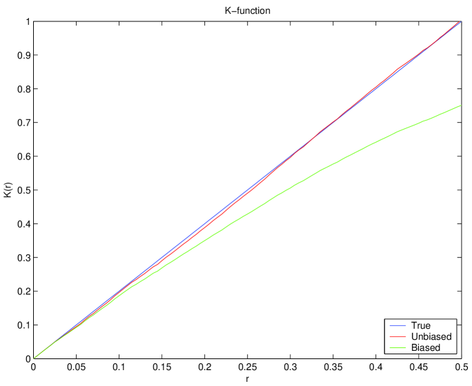
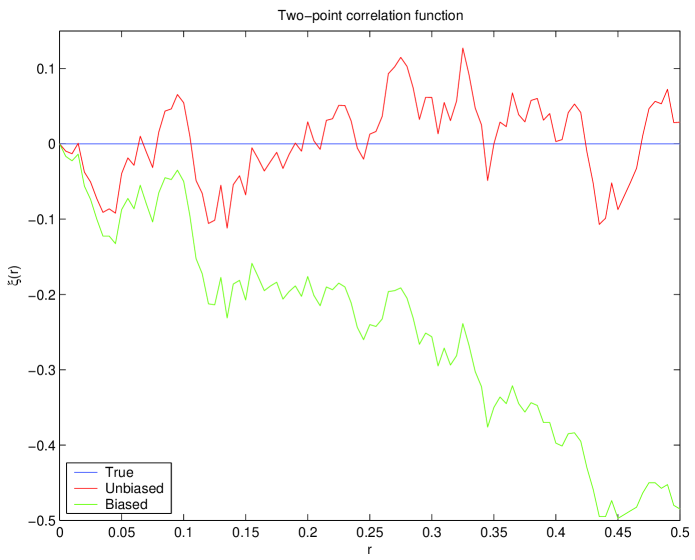
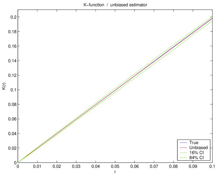
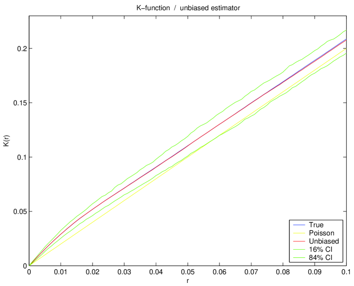
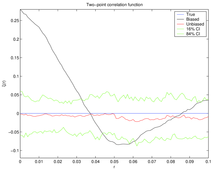
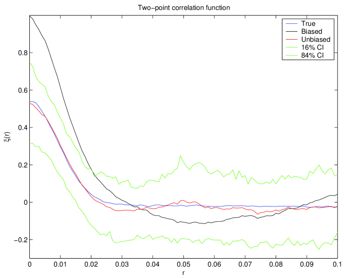
Figures 1-2 show that the mentioned biases are really significant also in the one-dimensional case considered here. As expected, the larger $r$ the larger the biases. This is due to the increasing number of points external to $W$ that, for increasing values of $r$, should be necessary to estimate both $K(r)$ and $\xi(r)$. Although not clearly visible in Fig. 2, $\bar{\xi}(r)$ presents a bias also when $r<h$. This is because in the computation of $\xi(r)$ only the points in the interval $[0,r+h]$ of length shorter than $2h$ can be considered.

Figure 1: Comparison of the biased estimator $\bar{K}(r)$ with the unbiased one $\widehat{K}(r)$ with adapted intensity $\lambda_{V}(r)$. The data used in the simulation consist of $200$ points drawn from a Poisson process in the interval $[0,1]$.

Figure 2: Comparison of the biased estimator $\bar{g}(r)$ with the unbiased one $\widehat{g}(r)$ with adapted intensity $\lambda_{S}(r)$. The data used in the simulation are the same of Fig. 1. $h=0.05$.

In Astronomy, especially in the field of the statistical analysis of the systems of galaxies, this edge-correction problem is well known. Various algorithms, mostly of Monte Carlo (MC) type, have been proposed for the three-dimensional case (e.g., see Hamilton 1993; Landy & Szalay 1993; Quashnock & Sein 1999; Pons-Bordería et al. 1999; Kerscher 1999; Kerscher et al. 2000; Martinez & Saar 2002, and references therein). Their conversion to the one-dimensional case is straightforward. However, the fact to work in the one-dimensional case allows us to follow the approach due to Stoyan & Stoyan (2000) which is a modification of the MC methods presented in Hamilton (1993) and Landy & Szalay (1993). In practice, the auxiliary random samples of points used in those papers are replaced by geometrical terms that result from exact integration. This permits to obtain more precise results since the quantities of interest are calculated and not only estimated as in the case of the MC techniques. Moreover, there is a remarkable benefit in the computational efficiency. In fact, in order to provide satisfactory results, the MC methods require the use of a number of auxiliary random samples much larger than the number of experimental points with obvious computational costs (see Martinez & Saar 2002).

We start from the unbiased rigid motion corrected estimators of $\lambda^{2}K(r)$ and $\lambda^{2}\xi(r)$:

$$\lambda^{2}\widehat{K}(r)=|W|\sum_{i=1}^{n}\sum_{j=1,j\neq i}^{n}p_{ij}^{-1}I_{r}(|x_{i}-x_{j}|),$$ (9)

where the weights $p_{ij}$ are given by

$$p_{ij}=\frac{|W\cap W_{x_{i}-x_{j}}|}{|W|}.$$ (10)

$W_{s}$ is the observing window shifted by the amount $s$. If $W$ is an interval, it is simply $|W\cap W_{x_{i}-x_{j}}|=|W|-|x_{i}-x_{j}|$. Similarly:

$$\lambda^{2}\widehat{\xi}(r)=\frac{|W|c(r)}{2}\sum_{i=1}^{n}\sum_{j=1,j\neq i}^{n}p_{ij}^{-1}k_{h}(r-|x_{i}-x_{j}|)-\lambda^{2}.$$ (11)

Here, $c(r)=2h/(r+h-\max[0,r-h])$ is a correcting factor for the values of $r$ for which $r-h$ goes negative (Guan 2006). A “naive” method used by many authors to obtain estimates of $K(r)$ and $\xi(r)$ is to set $\lambda^{2}=n^{2}/|W|^{2}$ and then to divide the estimators (9) and (11) by this quantity. However, the circumstance that $n/|W|$ is a good estimator of $\lambda$ does not necessarily implies that the same holds for $n^{2}/|W|^{2}$ with respect to $\lambda^{2}$. In fact, more is possible. As Hamilton (1993) and Landy & Szalay (1993) showed for $\xi(r)$ and Stoyan & Stoyan (2000) for $K(r)$, it is possible to reduce the mean squared error (${\rm MSE}$) if, instead of the naive classical estimator, adapted estimators for $\lambda$ are used. One particularity of these estimators is that they are different for $K(r)$ and $\xi(r)$ and depend on the distance $r$. They are denoted by $\lambda_{S}(r)$, for $\xi(r)$, and $\lambda_{V}(r)$, for $K(r)$. The index “$S$” refers to surface and “$V$” to volume (for more details, see Stoyan & Stoyan 2000). The expression for the two estimators is given by

$$\lambda_{S}(r)=\sum_{i=1}^{n}\frac{\@vec{1}_{W}(x_{i}-r)+\@vec{1}_{W}(x_{i}+r)}{2|W\cap W_{r}|},$$ (12)

and

$$\lambda_{V}(r)=\sum_{i=1}^{n}\frac{|W\cap[x_{i}-r,x_{i}+r]|}{2\int_{0}^{r}|W\cap W_{t}|dt},$$ (13)

with

$$\@vec{1}_{w}(x)=\left\{\begin{array}[]{ll}1&\textrm{\leavevmode\nobreak\ \leavevmode\nobreak\ if $x\in W$},\\ 0&\textrm{\leavevmode\nobreak\ \leavevmode\nobreak\ otherwise.}\end{array}\right.$$ (14)

Figures 1-2 show the remarkable improvement in the estimate of both $K(r)$ and $\xi(r)$.

3 Estimation of $K(r)$ and $\xi(r)$ in presence of gaps

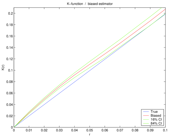
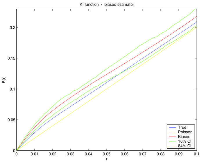
In practical applications, the edge effects are not the only problem. In fact, often the observing window is a union of intervals separated by gaps. In the spectra of quasars this is due to the presence of metal lines and strong Ly-$\alpha$ systems that can hidden portions of the Ly-$\alpha$ forest. Ignoring these gaps and taking erroneously the interval starting with the most left interval start-point to the most right interval endpoint as the observing window produces biased estimates. Clearly, the estimators will tend to report more clustering than really existing. The reason is simply that when the points within some given regions are removed, then this artificially creates separated groups of points that mimic the presence of clusters. As a consequence, an erroneous indication of clustering can happen even in the case of no-interaction or complete spatial randomness in the point pattern. On the other hand, if clustering or aggregation is really present, a higher degree of clustering than true may be obtained. These effects are clearly visible in Figs. 3-4 where the performance of the estimator $\bar{K}(r)$ is shown for a Poisson process, typically of complete random spatial patterns, and a Cox one that models spatial patterns with significant density fluctuations (Moller & Waagepetersen 2004).

In presence of gaps the unbiased estimators $\widehat{K}(r)$ and $\widehat{\xi}(r)$ and the intensities $\lambda_{V}(r)$ and $\lambda_{S}(r)$ can still be used. Here, however, a computational problem arises. In fact, although the computation of the quantities $|W\cap W_{x_{i}-x_{j}}|$, $\lambda_{S}(r)$ and $\lambda_{V}(r)$ needs only elementary mathematics, nevertheless it is impossible to give explicit formulas. For small $r$, a simple approximation is given by

$$|W\cap W_{r}|=L-(n_{w}+1)r,$$ (15)

where $L$ is the distance between the most left observation interval endpoint and the most right observation interval endpoint and $n_{w}$ is the number of gaps. For larger $r$, the exact algorithm presented in Appendix A can be used. As an alternative, the approximated but efficient algorithm based on a Fourier technique in Appendix B is proposed. After that, it is possible to compute $\lambda_{S}(V)$ and then $\widehat{\xi}(r)$. The computation of $\lambda_{V}(r)$ is more complicated and can be carried out by numerical integration. However a more efficient approach, based again on a Fourier technique, is described in Appendices B-C.

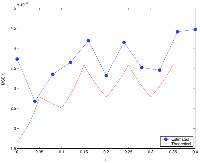
The excellent performance of the estimator $\widehat{K}(r)$ combined with the intensity $\lambda_{V}(r)$ is shown in Figs. 5-6 (to compare with Figs. 3-4). Figures. 7-8 show the results obtainable with $\widehat{\xi}(r)$ combined with $\lambda_{S}(r)$. The number of points used in this simulations is of the same order of that typically expected for the Ly-$\alpha$ lines in a single spectrum. In order to check if these results are consistent with what expected from the theory, in Fig. 9 the theoretical ${\rm MSE}_{\xi}(r)$ of the $\widehat{\xi}(r)$ estimator combined with $\lambda_{S}(r)$ for the experiment with the Poisson process used for Fig. 7 is compared with that estimated on the basis of $5000$ simulations; apart from the very small values of $r$, where the effects due to the bandwidth $h$ are more important, the agreement is reasonably good. Worth of note is the non-monotonic behavior of the two ${\rm MSE}$s that is directly linked to the fact that the observing window $W$ is constituted by disjoint segments. The equation used for ${\rm MSE}_{\xi}(r)$,

$${\rm MSE}_{\xi}(r)=\frac{\xi(r)+1}{2h\lambda^{2}|W\cap W_{r}|},$$ (16)

is due to Stoyan et al. (1993).

4 A practical application

In order to apply the discussed method and verify its reliability, we have used the best high resolution high signal-to-noise quasar spectra publicly available observed with the UVES spectrograph (Dekker et al. 2000) at the VLT telescope in the context of the ESO Large Programme “The Cosmic Evolution of the IGM” (Bergeron et al. 2004). In particular, we have chosen two examples of Ly-$\alpha$ forest contaminated by a large number of metal transitions: PKS0237-23 at $z_{\rm em}=2.233$ and PKS2126-158 at $z_{\rm em}=3.267$, for which the line blanketing due to the same Ly-$\alpha$ lines is more severe as the emission redshift is larger.

The quasar spectra have a resolution $R\simeq 45000$ and a signal-to-noise ratio in the Ly-$\alpha$ forests $S/N\simeq 80$ per pixel. They have been reduced with the pipeline of the instrument (version 2.1, Ballester et al. 2000) provided by ESO in the context of the data reduction package MIDAS. The continuum level was determined with a manual subjective method based on the selection of the regions free from clear absorption that are successively fitted with a spline polynomial of 3rd degree. The normalized spectra are then inspected to identify metal absorption systems with a particular attention to the transitions that fall in the Ly-$\alpha$ forest. Once the forest has been cleaned, the H i lines are fitted with Voigt profiles in the LYMAN context of the MIDAS reduction package. In order to increase the reliability of the fit parameters for the saturated Ly-$\alpha$ lines we used also the other unblended lines of the Lyman series falling in the observed spectral range. We excluded 1000 km s^-1 from the Ly-$\beta$ emission and 5000 km s^-1 from the Ly-$\alpha$ emission of the quasar to avoid associated absorbers and the proximity effect due to the quasar itself. Furthermore, we cut out of the spectra the regions occupied by the metal transitions and the Lyman limit systems (Ly-$\alpha$ lines with column density $N($HI$)\geq 10^{17}$ cm^-2) which could mask the presence of weaker lines in their velocity profiles (line blanketing). At the smallest scales the clustering properties are affected by the typical velocity width of the lines ($\sim 25-30$ km s^-1, e.g. Kim et al. 2001), for this reason we have merged the line pairs closer than $25$ km s^-1.

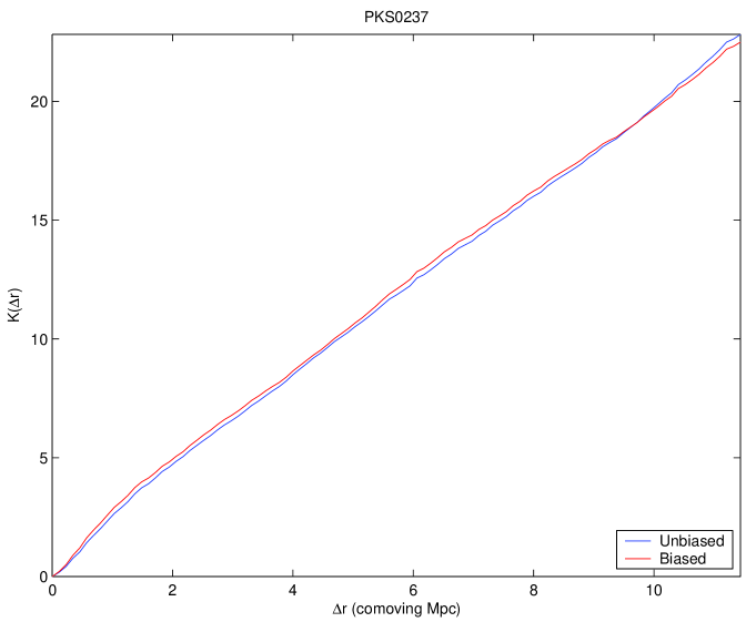
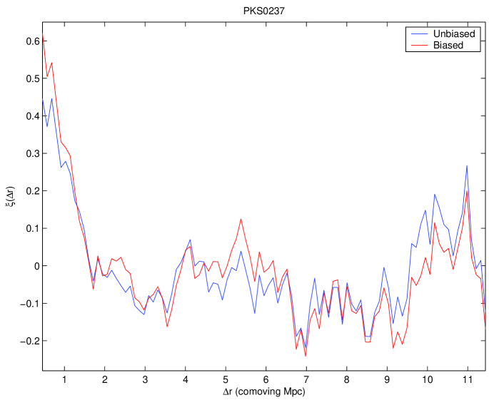
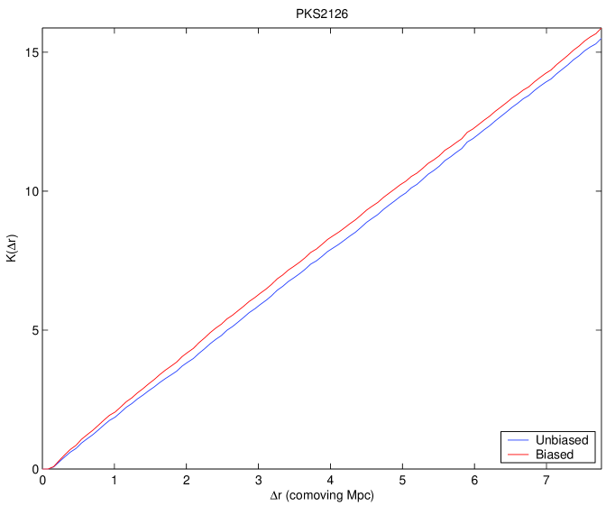
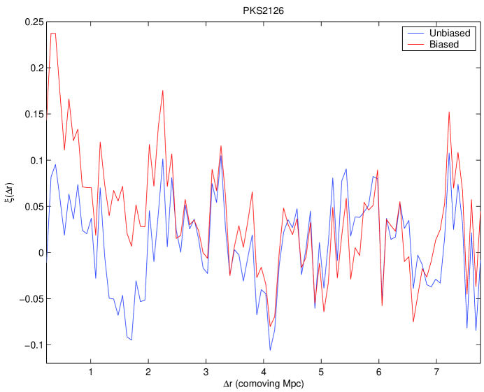
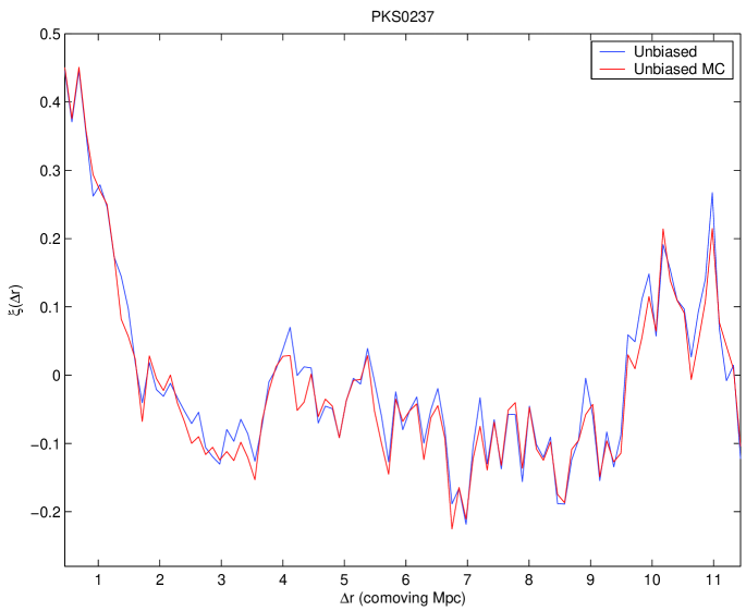
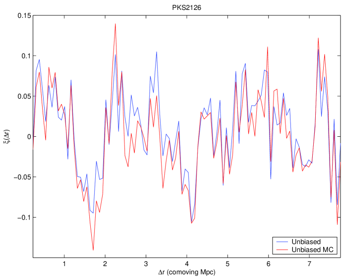
Figures 10-13 show $\widehat{K}(\Delta r)$ and $\widehat{\xi}(\Delta r)$ as a function of comoving spatial separation, $\Delta r$, for the Ly-$\alpha$ forest data of the objects PKS0237-23 and PKS2126-158. For PKS0237-23 the number of Ly-$\alpha$ lines is $191$ and the total length of gaps amounts to about $16\%$ of the interval spanned by $W$, whereas for PKS2126-158 these quantities are $300$ and $20\%$, respectively. For reference, the corresponding functions edge-corrected but evaluated without considering the gaps are also displayed. In both the cases, it is evident the stronger indication of clustering if the gaps are not taken into account. For the same experiment, Figs. 14-15 show the comparison between $\widehat{\xi}(\Delta r)$ and the estimate of the two-point correlation function obtained with the MC method by Landy & Szalay (1993). In this last case a number of $N_{D}=50$ data sets have been generated that contain a number of random samples equal to that of the original ones. $N_{D}$ has been chosen large enough that the mean of the estimated two-point correlation functions does not change significantly when more data sets are added. The good agreement is evident. However, if the computation of $\widehat{\xi}(\Delta r)$ takes a total of $1$-$2$ seconds of CPU time , the MC method requires a similar amount of time for each random sample. Now, if one takes into account that usually the bandwidth $h$ has to be determined by a trail and error approach, also with the limited size of the data sets here used, the computational advantage of the method presented in this paper is obvious. This is especially true if two or more lists of lines have to be analyzed at the same time (see below).

5 Multi-list analysis

Here, we briefly illustrate an additional benefit in using the estimator $\widehat{\xi}(r)$. In particular, the fact that it can be easily generalized for the estimation of a two-point correlation function when two or more lists of lines are available. The main problem is that, in an experimental context, the lists can have different characteristics concerning the covered spatial intervals and/or the total extension of the gaps. Hence, the naive estimator

$$\Xi(r)=\frac{1}{L}\sum_{l=1}^{L}\widehat{\xi}_{l}(r),$$ (17)

with $\widehat{\xi}_{l}(r)$ the estimate obtained from the $l$th data set, can provide unsatisfactory results since all the lists have the same importance in forming the final result. Some kind of weighting is necessary. In this respect, it has been proved (Ohser & Müecklich 2000) that the estimator

$$\widehat{\Xi}(r)=\frac{\sum_{l=1}^{L}|W\cap W_{r}|_{l}\leavevmode\nobreak\ \widehat{\xi}_{l}(r)}{\sum_{l=1}^{L}|W\cap W_{r}|_{l}}$$ (18)

provides an estimate of $\xi(r)$ with a smaller variance with respect to $\Xi(r)$ for each value of $r$. With the numerical techniques described in Sects. B-D, the implementation of the algorithm for the computation of $\widehat{\Xi}(r)$ is trivial. However, the characteristics and the performances of this estimator are beyond the scope of the present paper.

6 Conclusions

In this work we have analyzed possible sources of bias in the estimation of the second-order characteristics of the Ly-${\alpha}$ forest. In particular, the metallic and the strong Ly-$\alpha$ lines have been considered that can hidden part of the lines of interest. This may result in a severe bias of both the $K$-function and the two-point correlation function. Specifically, an erroneous indication of clustering can happen even in the case of no-interaction or complete spatial randomness in the line pattern or, if a clustering is really present, a higher degree of clustering than true can be obtained. In order to handle this problem, we have proposed a computational efficient method that has been implemented in two different algorithms; one that is able to provide exact results and the other one that is approximated but very fast. Its excellent performances have been validated through numerical simulations and an application to real data. We have also presented an extension of the method for the estimation of the two-point correlation function in the case of two or more lists of lines that have to be analyzed at the same time.

Figure 3: Mean and $68\%$ (i.e., $1$-$\sigma$) confidence interval for the biased estimator $\bar{K}(r)$, with periodic boundary conditions, obtained from $100$ realizations of a Poisson process with gaps. The data sets has been simulated by drawing $200$ points from a Poisson process in the interval $[0,1]$ and discharging those that are in subset $[0.20,0.25]\cup[0.30,0.35]\cup[0.50,0.55]\cup[0.70,0.75]\cup[0.80,0.85]$. For reference also the $K$-function of the Poisson process is shown (“true” line). Because of the imposed period boundary conditions, estimator $\bar{K}(r)$ is free from the edge effects.

Figure 4: The same as in Fig. 3 but for a Cox process simulated in the interval $[0,1]$ by taking the absolute value of a stationary Gaussian random field with a Gaussian correlation function whose dispersion is set to $0.01$. The Gaussian random fields have been generated under the hypothesis of periodic boundary conditions. Because of this, the line labeled “True”, that provides the mean value of the estimator $\bar{K}(r)$ with periodic boundary conditions, is free from the edge effects. This mean has been computed on the basis of $5000$ simulations with $W\equiv[0,1]$. For reference, also the $K$-function of a Poisson process is shown.

Figure 5: As in Fig. 3 but for the unbiased estimator $\widehat{K}(r)$ and the adapted intensity $\lambda_{V}(r)$.

Figure 6: As in Fig. 4 but for the unbiased estimator $\widehat{K}(r)$ and the adapted intensity $\lambda_{V}(r)$.

Figure 7: As in Fig. 3 but for the unbiased estimator $\widehat{\xi}(r)$ and the adapted intensity $\lambda_{S}(r)$. $h=0.01$.

Figure 8: As in Fig. 4 but for the unbiased estimator $\widehat{\xi}(r)$ and the adapted intensity $\lambda_{S}(r)$. $h=0.005$.

Figure 9: Estimated ${\rm MSE}_{\xi}(r)$ (calculated for eleven values of $r$) vs. the theoretical one for the experiment in Fig. 7. Notice the non-monotonic behavior of the two functions that is directly linked to the fact that the observing window $W$ is constituted by disjoint segments.

Figure 10: $\widehat{K}(\Delta r)$ for the data of PKS0237-23 when the gaps due to the metal and the strong Ly-$\alpha$ lines are taken into account (unbiased estimator) as a function of the comoving spatial separation, $\Delta r$. The largest value of $\Delta r$ in the figure corresponds to about $5\%$ the interval spanned by this quantity. The total extension of gaps amount to about $16\%$ of spatial interval covered by $W$. For reference, the same estimate is shown when gaps are neglected (biased estimator).

Figure 11: $\widehat{\xi}(\Delta r)$ for the data of PKS0237-23 when the gaps due to the metal and the strong Ly-$\alpha$ lines are taken into account (unbiased estimator) as a function of the comoving spatial separation, $\Delta r$. The largest value of $\Delta r$ in the figure corresponds to about $5\%$ the interval spanned by this quantity. The total extension of gaps amount to about $16\%$ of spatial interval covered by $W$ and $h=0.001$ in the same units. For reference, the same estimate is shown when gaps are neglected (biased estimator).

Figure 12: $\widehat{K}(\Delta r)$ for the data of PKS2126-158 when the gaps due to the metal and the strong Ly-$\alpha$ lines are taken into account (unbiased estimator)as a function of the comoving spatial separation, $\Delta r$. The largest value of $\Delta r$ in the figure corresponds to about $5\%$ the interval spanned by this quantity. The total extension of gaps amount to about $20\%$ of spatial interval covered by $W$. For reference, the same estimator is shown when gaps are neglected (biased estimator).

Figure 13: $\widehat{\xi}(\Delta r)$ for the data of PKS2126-158 when the gaps due to the metal and the strong Ly-$\alpha$ lines are taken into account (unbiased estimator) as a function of the comoving spatial separation, $\Delta r$. The total extension of gaps amount to about $20\%$ of spatial interval covered by $W$ and $h=0.001$ in the same units. For reference, the same estimator is shown when gaps are neglected (biased estimator).

Figure 14: $\widehat{\xi}(\Delta r)$ for the data of PKS0237-23 when the gaps due to the metal and the strong Ly-$\alpha$ lines are taken into account (unbiased estimator) as a function of the comoving spatial separation, $\Delta r$. The largest value of $\Delta r$ in the figure corresponds to about $5\%$ the interval spanned by this quantity. The total extension of gaps amount to about $16\%$ of spatial interval covered by $W$ and $h=0.001$ in the same units. For reference, the result provided by the MC method by Landy & Szalay (1993) is also shown (unbiased MC estimator).

Figure 15: $\widehat{\xi}(\Delta r)$ for the data of PKS2126-158 when the gaps due to the metal and the strong Ly-$\alpha$ lines are taken into account (unbiased estimator) as a function of the comoving spatial separation, $\Delta r$. The largest value of $\Delta r$ in the figure corresponds to about $5\%$ the interval spanned by this quantity. The total extension of gaps amount to about $16\%$ of spatial interval covered by $W$ and $h=0.001$ in the same units. For reference, the result provided by the MC method by Landy & Szalay (1993) is also shown (unbiased MC estimator).

Appendix A An exact method to compute $|W\cap W_{r}|$

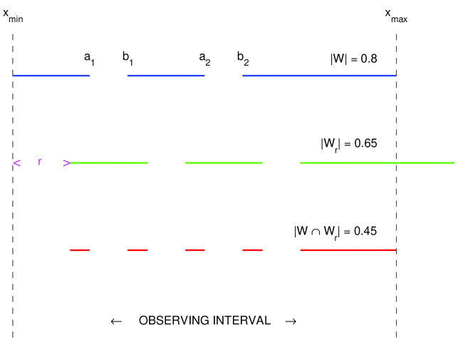
The following presents a pseudo-code that implements an exact algorithm for the computation of $|W\cap W_{r}|$ for a window $W$ with gaps. It is assumed that the observing window $W$ lies in the interval $[x_{\rm min},x_{\rm max}]$ and has $n_{k}$ gaps $[a_{k},b_{k}]$ for $k=1,...,n_{k}$ with

$$x_{\rm min}=b_{0}<a_{1}<b_{1}<...<a_{n_{k}}<b_{n_{k}}<a_{n_{k}+1}=x_{\rm max}.$$

Fig. 16 shows the situation for the case $n_{k}=2$.

The algorithm considers all combinations of the intervals between the gaps, determines the lengths of their intersections and sums up. The wanted length $|W\cap W_{r}|$ is denoted by $s$.

Figure 16: Example of an observing window $W$ with two gaps, its shifted version $W_{r}$ and the intersection $W\cap W_{r}$. The window lengths are given in units of the observing interval $x_{\rm max}-x_{\rm min}$. r=0.15 in the same units.

% input:
% $r$ $\longrightarrow$ interpoint distance
%

% initialization of indices:
$s=0;$
$i1=1;$
$i2=1;$

% fix the shifted interval:
$y1=b[i1-1]+r;$
$y2=a[i1]+r;$
if $y2>x_{\rm max}$ then $y2=x_{\rm max};$ end
% fix the original interval:
$z1=b[i2-1];$
$z2=a[i2];$

% compute the length of the intersections
while $(i1\leq n_{k}+1)$ and $(y1<x_{\rm max})$ do
          if $z2<y2$ then
                  if $z2>y1$ then
                           if $z1>y1$ then
                                    $s=s+z2-z1;$
                           else
                                    $s=s+z2-y1;$
                           end
                           $i2=i2+1;$
                           $z1=b[i2-1];$
                           $z2=a[i2];$
                  end
          else if $z1<y2$ then
                           if $z1>y1$ then
                                    $s=s+y2-z1;$
                           else
                                    $s=s+y2-y1;$
                           end
                           $i1=i1+1;$
                           $y1=b[i1-1]+r$;
                           if $i1\leq n_{k}+1$ then
                                    $y2=a[i1]+r$;
                                    if $y2>x_{\rm max}$ then
                                            $y2=x_{\rm max}$;
                                    end
                           end
                  end
          end
end
return $s$

Appendix B An approximate fast method to compute $|W\cap W_{r}|$

The method presented in the previous section provides an exact value of $|W\cap W_{r}|$. If the computing time is of concern, a more efficient, although approximated method, is possible. The idea is to consider the observing window $W$ as a function $\mathcal{W}(x)$ in $\mathbb{R}$ defined in the domain $(-\infty,+\infty)$. When $x\in[x_{\rm min},x_{\rm max}]$, then $\mathcal{W}(x)=0$ if $x$ belongs to a gap, $\mathcal{W}(x)=1$, otherwise. If $x\notin[x_{\rm min},x_{\rm max}]$, it is $\mathcal{W}(x)=0$.

It is not difficult to realize that, for a fixed $r^{*}$, $\gamma(r^{*})\equiv|W\cap W_{r^{*}}|$ is given by

$$\gamma(r^{*})=\int_{-\infty}^{+\infty}\mathcal{W}(x)\mathcal{W}(x+r^{*})dx.$$ (19)

When $r^{*}$ is made to change in the interval $(-\infty,+\infty)$, this equation provides the autocorrelation function of $\mathcal{W}(x)$. Hence,

$$\gamma(r)={\rm IFT}\left\{{\rm FT}[\mathcal{W}(x)]\times({\rm FT}[\mathcal{W}(x)])^{\prime}\right\}.$$ (20)

The symbol “$\leavevmode\nobreak\ {}^{\prime}\leavevmode\nobreak\$” means complex conjugation, whereas ${\rm FT}$ and IFT denote the Fourier transform and the inverse Fourier transform, respectively.

An efficient implementation of Eq. (20) requires the interval $[x_{\rm min},x_{\rm max}]$ be discretized in a set of $N_{b}$ bins. In the case of the estimator $\widehat{\xi}(r)$, this does not represent a true limit since it is a function that is computed on spatial bins of length $2h$ (see Eq. (11)). The value of $N_{b}$ to use in the discretization depends on factors as the extension of the gaps, the number of points and the range of distance $r$ of interest (see also below). In any case, this is not a critical quantity. In the numerical experiments presented in the previous sections, $N_{b}=5000$ is sufficient to obtain results almost indistinguishable from those obtainable with an exact approach. However, even values of $N_{b}$ much larger than this one (e.g., $10^{5}$) determine only a limited increase of the computational burden.

If $\@vec{w}$ is an array of length $2N_{b}$, with its central $N_{b}$ elements containing function $\mathcal{W}(x)$ in the interval $x\in[x_{\rm min},x_{\rm max}]$ sampled on a discrete grid, then

$$\@vec{\gamma}\approx{\rm IDFT}\left\{{\rm DFT}[\@vec{w}]\odot({\rm DFT}[\@vec{w}])^{\prime}\right\}\times\Delta x.$$ (21)

Symbol “$\odot$” indicates the point-wise multiplication, $\Delta x$ is the sampling step and ${\rm DFT}$ and IDFT denote the fast discrete Fourier transform and the fast inverse discrete Fourier transform, respectively. The computational benefit of this approach is evident since the first $N_{b}$ elements of $\@vec{\gamma}$ contain the values of $\gamma(r)$ for $0\leq r\leq(x_{\rm max}-x_{\rm min})$. The fact of using an array $\@vec{w}$ of length $2N_{b}$ corresponds to a zero-padding operation to avoid the aliasing effects typical of the discrete Fourier transform. Array $\@vec{\gamma}$ can be used to compute the weights $\{p_{ij}\}$ in Eq. (11).

Appendix C An approximate fast method to compute $\lambda_{S}(r)$ and $\lambda_{V}(r)$

As shown by Eqs. (9)-(11), the estimators $\widehat{K}(r)$ and $\widehat{\xi}(r)$ require the intensities $\lambda_{V}(r)$ and $\lambda_{s}(r)$. Again, the computation can be done with an exact algorithm as in Appendix A. As an alternative, an approximative but very efficient Fourier based algorithm is possible that, similarly to Appendix B, requires the discretization of the interval $[x_{\rm min},x_{\rm max}]$ in a set of $N_{b}$ bins.

Once $\@vec{\gamma}$ has been calculated, the computation of $\lambda_{S}(r)$ is a trivial operation. In fact, it is sufficient to check whether the elements of the array $\@vec{w}$ that correspond to $x_{i}-r$ and $x_{i}+r$ are equal to $0$ or to $1$. The situation is more complex for $\lambda_{V}(r)$ because of the terms $\theta(r)=\sum_{i=1}^{n}|W\cap[x_{i}-r,x_{i}+r]|$ and $\epsilon(r)\equiv 2\int_{0}^{r}|W\cap W_{t}|dt$.

For $\theta(r)$, the basic idea is to identify the term $[x_{i}-r,x_{i}+r]$ as a function $w_{i}^{r}(x)$ such as $w_{i}^{r}(x)=1$ for $x\in[x_{i}-r,x_{i}+r]$, $w_{i}^{r}(x)=0$ otherwise. The reason is that in this way $w_{i}^{r}(x)$ can be expressed in the convolution form

$$w_{i}^{r}(x)=\int_{-\infty}^{+\infty}I_{r}(|x|)\delta(x-x_{i})dx,$$ (22)

where $\delta(x)$ is the classic impulse function. Then, for a given $r^{*}$, it is possible to write $\theta(r^{*})$ in the form

$$\theta(r^{*})=\int_{-\infty}^{+\infty}\mathcal{W}(x)\sum_{i=1}^{n}w_{i}^{r^{*}}(x)dx.$$ (23)

Now, a discrete approximation of $\theta(r^{*})$ is provided by

$$\theta(r^{*})\approx{\rm SUM}\left[\@vec{w}\odot{\rm IDFT}\left\{{\rm DFT}[\@vec{I}_{r^{*}}]\odot{\rm DFT}[\@vec{x}]\right\}\right]\times\Delta x.$$ (24)

${\rm SUM}[\@vec{z}]$ is the operator that sums up all the elements of the array $\@vec{z}$, $\@vec{x}$ is an $N_{b}+N_{0}$ array that in its central $N_{b}$ elements contains the number of points in each of the bins of $W$, whereas $\@vec{I}_{r}$ is a $N_{b}+N_{0}$ array containing the discretized version of the function $I_{r}[.]$ stored in wraparound order with $N_{0}$ providing the number of zero-pads necessary to avoid the aliasing effect due to the DFT. Here, also the array $\@vec{w}$ has size $N_{b}+N_{0}$. The term ${\rm DFT}[\@vec{I}_{r^{*}}]$ has not necessarily to be calculated numerically since an analytical expression is available (e.g., see Briggs & Henson 1996). In principle, $N_{b}$ should be chosen large enough that each entry of the array $\@vec{x}$ is either $0$ or $1$. However, from our numerical experiments its comes out that a value of $N_{b}$ such as $5$-$10$ bins correspond to the bandwidth $h$ is sufficient to obtain satisfactory results.

For a given $r^{*}$, an approximation of $\epsilon(r^{*})$ can be obtained from the array $\@vec{\@vec{\gamma}}$ by means of

$$\epsilon(r^{*})\approx 2\times{\rm SUM}[\@vec{\@vec{\gamma}}(1:i_{r^{*}})]\times\Delta x.$$ (25)

$(1:i_{r^{*}})$ indicates the indices of the elements of the array to sum up and $i_{r}$ is the index of the bin corresponding to the distance $r$.

Appendix D An approximated fast method to compute $\lambda^{2}\widehat{\xi}(r)$ and $\lambda^{2}\widehat{K}(r)$

In the previous appendices some efficient numerical methods have been presented to compute $|W\cap W_{r}|$ and $\lambda_{S}(r)$. These are some of the ingredients for the computation of the function $\widehat{\xi}(r)$ that, however, requires also the total number, $N_{h}(r)$, of pairs with a distance in the range $[r-h,r+h]$. The simplest method to obtain this last quantity consists in counting. In the one-dimensional case, especially for limited data sets and/or small $r$, this represents the most efficient approach (we have used it in our numerical experiments). In the case of large data sets, an alternative method based on a Fourier approach is possible, that permits to obtain $N_{h}(r)$ without the necessity to compute the distance between the points (see also Szapudi et al. 2005).

The basic idea is that two points $x_{i}$ and $x_{j}$ ($x_{i}<x_{j}$) have a distance in the range $[r-h,r+h$] if $x_{j}\in[x_{i}+r-h,x_{i}+r+h]$. Now, this condition can be expressed in the equivalent form

$$2h\int_{-\infty}^{+\infty}k_{h}(x-x_{i}-r)\delta(x-x_{j})dx=1.$$ (26)

A similar expression holds when $x_{i}>x_{j}$. Hence, if $r>h$, $N_{h}(r)$ is given

$$N_{h}(r)=2h\sum_{i=1}^{n}\sum_{j=1}^{n}\int_{-\infty}^{+\infty}k_{h}(|x-x_{i}|-r)\delta(x-x_{j})dx.$$ (27)

When $r\leq h$, this number has to be subtracted by the number $n$ of points (to avoid self-pairing). If discretized, for a fixed $r^{*}$, this equation takes the form,

$$N_{h}(r^{*})\approx{\rm SUM}\left[\@vec{x}\odot{\rm IDFT}\left\{{\rm DFT}[\@vec{k}_{h}^{r^{*}}]\odot{\rm DFT}[\@vec{x}]\right\}\right],$$ (28)

where $\@vec{k}_{h}^{r^{*}}$ is the discretized form of the function $2hk_{h}(x-r^{*})$ stored in wraparound order. At this point, the computation of $\widehat{\xi}(r)$ should require the calculation of the weights $\{p_{ij}\}$ that depend on the quantities $\{|W\cap W_{x_{i}-x_{j}}|\}$. In their turn, these quantities depend on the distances $\{|x_{i}-x_{j}|\}$ that are not available. However, if $r\gg h$ (a typical situation of interest), from Eq. (11) it is

$$\frac{|W|}{|W\cap W_{x_{i}-x_{j}}|}k_{h}(|x_{i}-x_{j}|-r)\approx\frac{|W|}{|W\cap W_{r}|}k_{h}(|x_{i}-x_{j}|-r).$$ (29)

With this approximation the quantity $\lambda^{2}\widehat{\xi}(r)$ is given by

$$\lambda^{2}\widehat{\xi}(r^{*})=\frac{|W|^{2}c(r^{*})}{2|W\cap W_{r^{*}}|}N_{h}(r^{*}).$$ (30)

The denominator of this expression can be obtained from $\@vec{\gamma}$.

In Eq. (29), the term ${\rm DFT}[\@vec{k}_{h}^{r^{*}}]$ can be computed without actually performing the DFT operation if the array $\@vec{\kappa}_{h}^{0}\equiv{\rm DFT}[\@vec{k}_{h}^{0}]$ is available. In fact, it is

$$\@vec{\kappa}_{h}^{r^{*}}=\@vec{\kappa}_{h}^{0}\odot{\rm e}^{-\iota 2\pi i_{r^{*}}[0,1,\ldots,N-1]/N},$$ (31)

with $\iota\equiv\sqrt{-1}$, $i_{r}$ the index of the bin corresponding to the distance $r$, and $N$ the length of the array $\@vec{\kappa}_{h}^{0}$.

With arguments similar to those presented above, it is possible to show that, if $N(r^{*})$ is the total number of pairs with distance less or equal to a fixed $r^{*}$, then

$$N(r^{*})\approx{\rm SUM}\left[\@vec{x}\odot{\rm IDFT}\left\{{\rm DFT}[\@vec{I}_{r^{*}}]\odot{\rm DFT}[\@vec{x}]\right\}\right]-n,$$ (32)

and

$$\lambda^{2}\widehat{K}(r^{*})\approx\frac{|W|^{2}}{|W\cap W_{r}|}N(r^{*}).$$ (33)

References

- Ballester et al. (2000) Ballester, P., Modigliani, A., Boitquin, O., et al. 2000, ESO The Messenger, 101, 31
- Bergeron et al. (2004) Bergeron, J., Petitjean, P., Aracil, B., et al. 2004, ESO The Messenger, 118, 40
- Bi & Davidsen (1997) Bi, H.-G., & Davidsen, A. F. 1997, ApJ, 479, 523
- Briggs & Henson (1996) Briggs, W.L., & Henson, V.E. 1996, Applied Numerical Mathematics, 20, 1
- Cen et al. (1994) Cen, R., Miralda-Escudé, J., Ostriker, J.P., & Rauch, M. 1994, ApJ, 437, L83
- Cristiani et al. (1997) Cristiani, S., D’Odorico, S., D’Odorico, V., et al. 1997, MNRAS, 285, 209
- Davé et al. (1997) Davé, R., Hernquist, L., Weinberg, D.H., & Katz, N. 1997, ApJ, 477, 21
- Dekker et al. (2000) Dekker, H., D’Odorico, S., Kaufer, A., Delabre, B., & Kotzlowski, H. 2000, SPIE, 4008, 534
- D’Odorico et al. (2006) D’Odorico, V., Viel, M., Saitta, F., et al. 2006, MNRAS, 372, 1333
- Guan (2006) Guan Y. 2006, Statistics and Probability Letters, submitted
- Hamilton (1993) Hamilton A.J.S. 1993, ApJ, 417, 19
- Hernquist et al. (1996) Hernquist, L., Katz, N., Weinberg, D.H., & Miralda-Escudé, J. 1996, ApJ, 457, L51
- Kerscher (1999) Kerscher, M. 1999, A&A, 343, 333
- Kerscher et al. (2000) Kerscher, M., Szapudi, I., & Szalay, A. 2000, ApJ, 535, L13
- Kim et al. (2001) Kim, T.-S., Cristiani, S., & D’Odorico, S. 2001, A&A, 373, 757
- Kim et al. (2002) Kim, T.-S., Carswell, R.F., Cristiani, S., D’Odorico S., & Giallongo, E. 2002, MNRAS, 335, 555
- Landy & Szalay (1993) Landy ,S.D., & Szalay, A.S. 1993, ApJ, 412, 64
- Lu et al. (1996) Lu, L., Sargent, W.L.W., Womble, D.S., & Takada-Hidai, M. 1996, ApJ, 472, 509
- Martinez & Saar (2002) Martinez, V.J., & Saar, E. 2002, Statistics of the Galaxy Distribution (Boca Raton: Chapman & Hall/CRC press)
- Martínez et al. (2005) Martínez, V.J., Starck, J.L., Saar, et al. 2005, ApJ, 634, 744
- Machacek et al. (2000) Machacek, M. E., Bryan, G. L., Meiksin, A., Anninos, P., Thayer, D., Norman, M., & Zhang, Y. 2000, ApJ, 532, 118
- Miralda-Escudé et al. (1996) Miralda-Escudé, J., Cen, R., Ostriker, J.P., & Rauch, M. 1996, ApJ, 471, 582
- Moller & Waagepetersen (2004) Moller, J., & Waagepetersen, R.P. 2004, Statistical Inference and Simulation for Spatial Point Processes (Boca Raton: Chapman & Hall/CRC press)
- Ohser & Müecklich (2000) Ohser, J., & Müecklich, F. 2000, Statistical Analysis of Microstructures in Materials Science (Chichester: Wiley)
- Pons-Bordería et al. (1999) Pons-Bordería, M.J., Martinez, V.J., Stoyan, D., Stoyan, H., & Saar, E. 1999, ApJ, 523, 480
- Quashnock & Sein (1999) Quashnock, J.M., & Stein, M.L. 1999, ApJ, 515, 506
- Rauch et al. (2005) Rauch, M., Becker, G.D., Viel, M., Sargent, et al. 2005, ApJ, 632, 58
- Sargent et al. (1980) Sargent, W.L.W., Young, P.J., Boksenberg, A., & Tytler, D. 1980, ApJS, 42, 41
- Stoyan et al. (1993) Stoyan, D., Bertram, U. & Wndrock, H. 1993, Annals of the Institute of Statistical Mathematics 45, 211.
- Stoyan & Stoyan (2000) Stoyan, D., & Stoyan H. 2000, Scandinavian Journal of Statistics, 27, 641
- Szapudi et al. (2005) Szapudi, I., Pan, J., Prunet, S., & budavari, T. 2005, ApJ, 631, L1
- Theuns, Leonard & Efstathiou (1998) Theuns, T., Leonard, A., & Efstathiou, G. 1998, MNRAS, 297, L49
- Zhang et al. (1995) Zhang, Y., Anninos, P., & Norman, M.L. 1995, ApJ, 453, L57
- Zhang et al. (1997) Zhang, Y., Anninos, P., Norman, M.L., & Meiksin, A. 1997, ApJ, 485, 496