Efficient Bayesian inference for multimodal problems in cosmology

Abstract

Bayesian model selection provides the cosmologist with an exacting tool to distinguish between competing models based purely on the data, via the Bayesian evidence. Previous methods to calculate this quantity either lacked general applicability or were computationally demanding. However, nested sampling (Skilling 2004), which was recently applied successfully to cosmology by Muhkerjee et al. 2006, overcomes both of these impediments. Their implementation restricts the parameter space sampled, and thus improves the efficiency, using a shrinking ellipsoidal bound in the $n$-dimensional parameter space encompassing parameter samples above a decreasing likelihood value. However, if the likelihood function contains any multi-modality, separated over a significant portion of the parameter space then the ellipse is prevented from constraining the sampling region by less than the distance between the likelihood peaks. In this paper we introduce a method of clustered nested sampling whereby ellipsoidal clusters can form on any peaks identified –thus improving the efficiency by a factor which is equal to the ratio of the volumes enclosed by the set of small clustered ellipsoids and the large single ellipse that would necessarily be required without clustering. In addition we have implemented a method for determining the expectation and variance of the final evidence value without the need to use sampling error from repetitions of the algorithm ; this further reduces the computational load by at least an order of magnitude. We have applied our algorithm to a pair of toy models and one cosmological example where we demonstrate that the number of likelihood evaluations required is $\sim$ 4$\%$ of that necessary for using previous algorithms. We have produced a Fortran library containing our routines which can be called from any sampling code, in addition for convenience we have incorporated it into the popular CosmoMC code as CosmoClust. Both are available for download at www.mrao.cam.ac.uk/software/cosmoclust.

1 Introduction

Bayesian inference has become an invaluable tool in analysing cosmological datasets to place constraints on model parameters. However the more fundamental question of model selection, naturally incorporated in the Bayesian framework by the evidence, has been under-utilised in cosmology. Impeded until recently by the high computational cost of methods such as thermodynamic integration, progress has now been made with the advent of nested sampling (Skilling, 2004), targeted solely at efficient calculation of the evidence but also capable of providing posterior inferences. This method has recently been applied to cosmological problems by Mukherjee et al. (2006) allowing model selection on feasible timescales, typical of Markov Chain Monte Carlo (MCMC) parameter estimation. Their algorithm uses an elliptical bound to restrict the prior around the maximum likelihood peak in the posterior and thus improves the acceptance ratio and efficiency. While this method can be used for the majority of cosmological applications, where posteriors are generally uni-modal, there are examples where this is not so. In this paper we describe a clustering nested sampler which is capable of detecting and isolating multiple peaks in the posterior, fitting separate ellipsoidal bounds around each and making considerable savings in computational load when compared to a single ellipse. In addition we have implemented an improved error calculation (Skilling, 2004) on the final evidence result which produces a mean and standard error in one calculation, eliminating the need for multiple runs.

2 Bayesian Inference

A Bayesian analysis provides a coherent approach to the estimation of a set of model parameters $\mathbf{\Theta}$ and, crucially in determining which model, $M$, best describes the data, $\mathbf{D}$. Bayes’ theorem states that

$$P(\mathbf{\Theta}|\mathbf{D},M)=\frac{P(\mathbf{D}|\mathbf{\Theta},M)P(\mathbf{\Theta}|M)}{P(\mathbf{D}|M)},$$ (1)

where $P(\mathbf{\Theta}|\mathbf{D},M)$ is the posterior probability distribution, $P(\mathbf{D}|\mathbf{\Theta},M)\equiv\mathcal{L}$ the likelihood, $P(\mathbf{\Theta}|M)\equiv\pi$ the prior, $P(\mathbf{D}|M)\equiv\mathcal{Z}$ the Bayesian evidence.

Typically, the posterior is generated via a Metropolis-Hastings algorithm with MCMC sampling, where at equilibrium the chain contains a set of samples from parameter space distributed with the posterior probability distribution. In the Bayesian framework all of the inference is contained in the final multi-dimensional posterior, which can be marginalised over each parameter to obtain constraints. The Bayesian evidence is represented by the overall normalisation of this posterior. The evidence is large in models which have a high likelihood over a large proportion of the prior parameter space so that we can consider the evidence to be the average of the likelihood divided by the prior. As such it forms the integral, over the $n$-dimensional parameter space

$$\mathcal{Z}=\int{\mathcal{L}(\mathbf{\Theta})\pi(\mathbf{\Theta})}d^{n}\mathbf{\Theta}.$$ (2)

Thus a model containing a large number of parameters for which only a narrow region of the prior is likely will have a low evidence and vice versa, providing a natural mechanism to limit the complexity of cosmological models and elegantly incorporating Ockham’s razor.

A standard scenario in Bayesian model selection would require the computation of evidences for two models A and B. The difference of log-evidences $\ln\mathcal{Z}_{A}-\ln\mathcal{Z}_{B}$, also called the Bayes factor then quantifies how well A may fit the data when compared with model B. Jeffreys (1961) provides a scale on which we can make qualitative conclusions based on this difference: $\Delta\mbox{ln}\mathcal{Z}<1$ is not significant, $1<\Delta\mbox{ln}\mathcal{Z}<2.5$ significant, $2.5<\Delta\mbox{ln}\mathcal{Z}<5$ strong and $\Delta\mbox{ln}\mathcal{Z}>5$ decisive.

The prior dependence of the evidence requires that the entire parameter space is adequately sampled, the MCMC method described above moves rapidly through parameter space toward areas of high likelihood leaving the majority of the surrounding prior heavily under sampled. This is sufficient to generate parameter constraints where regions close to the peak of the posterior are most important, but it radically over estimates the evidence due to under sampling of regions of low likelihood. In order to sample more uniformly the method of thermodynamic integration has previously been implemented (see e.g Hobson et al. 2003; Slosar et al. 2003) and used successfully by a number of authors (Niarchou et al. 2004, Basset et al. 2004, Mukherjee et al. 2006, Trotta 2005, Beltran et al. 2005, Bridges et al. 2006) in computing the evidence. Thermodynamic integration uses MCMC to draw samples not from the posterior directly but from $\mathcal{L}^{\lambda}\pi$ where $\lambda$ is the inverse temperature and is raised from $\approx 0$ to $1$. For low values of $\lambda$ peaks in the posterior are sufficiently flattened to allow improved mobility of the chains over the entire prior range. Typically it is possible to obtain accuracies of within 0.5 units in log-evidence via this method however this does require of order $10^{6}$ samples per chain (with around 10 chains required to determine a sampling error) making it at least an order of magnitude more costly than the sampling needed for parameter estimation.

3 Nested sampling

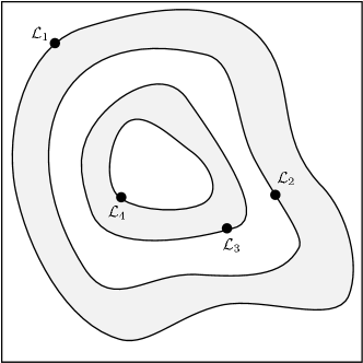
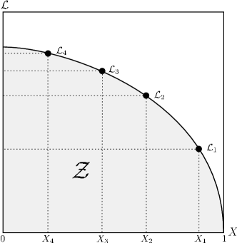
Nested sampling is computationally more efficient as it transforms the integral in Eqn. 2 to a single dimension by a suitable re-parameterisation in terms of the prior mass $X$. This mass can be divided into elements $dX=\pi(\mathbf{\Theta})d^{N}\mathbf{\Theta}$ which can be combined in any order to give say

$$X(\lambda)=\int_{\mathcal{L\left(\mathbf{\Theta}\right)>\lambda}}\pi(\mathbf{\Theta})d^{N}\mathbf{\Theta},$$ (3)

the prior mass covering all likelihoods above the iso-likelihood curve $\mathcal{L}=\lambda$. We also require the function $\mathcal{L}(X)$ to be a singular decreasing function (which is trivially satisfied for most posteriors) so that using sampled points we can estimate the evidence via the integral:

$$\mathcal{Z}=\int_{0}^{1}{\mathcal{L}(X)}dX.$$ (4)

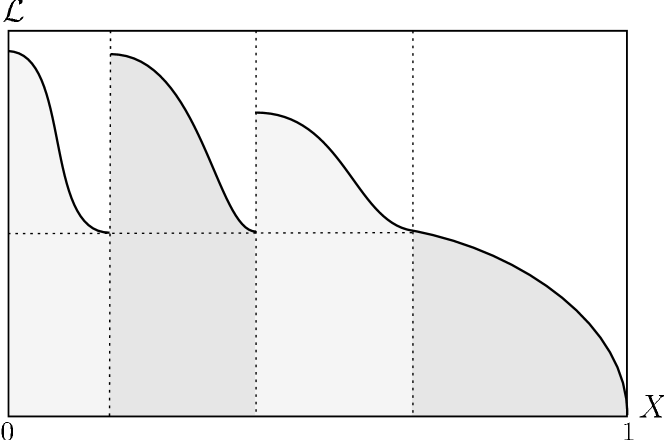
An example of a posterior in two dimensions and its associated function $\mathcal{L}(X)$ is shown in Fig. 1.

Figure 1: Cartoon illustrating the posterior of a two dimensional problem (a) and the transformed $\mathcal{L}(X)$ function (b) where the prior masses $X_{i}$ are associated with each likelihood $\mathcal{L}_{i}$.

The transformed integral is dominated by a relatively small region of the prior containing the majority of the posterior mass. For efficient sampling the division of the prior elements should not be linear but geometric:

$$X_{0}=1,X_{1}=t_{1}X_{0},\>\ldots\>X_{i}=t_{i}X_{i-1},\>\ldots\>X_{m}=0$$ (5)

where we would desire a largely constant $t_{i}$; the procedure for nested sampling ensures just that.

The method is then to draw an initial set of $N$ active samples uniformly from the full prior $[0,X_{0}=1]$. The samples are ordered in terms of likelihood, the smallest of which, $\mathcal{L}_{0}$ is removed from the active set. The prior is then reduced according to Eqn. 5 so that the region sampled becomes $[0,X_{1}]$ where $X_{1}=t_{1}X_{0}$, a point is then found to replenish the active set subject to the criterion that its likelihood $>\mathcal{L}_{0}$. This sampling/replenishment cycle is then repeated until the entire prior has been traversed. The algorithm thus travels through nested shells of likelihood as the prior mass is reduced. At this point the evidence is approximated by a numerical integration routine such as the trapezoid rule:

$$\mathcal{Z}=\sum_{i=1}^{N}\mathcal{L}_{i}\frac{(X_{i-1}-X_{i+1})}{2}.$$ (6)

The method described above ensures that the $t_{i}$ have the distribution $P(t_{i})=Nt_{i}^{N-1}$, allowing them to be statistically assigned. This does introduce an uncertainty, but it is possible to quantify this accurately and relate it to the final $\mathcal{Z}$. If we could assign each $X_{i}$ exactly then the only error would be due to the discretisation of the integral which, given sufficient points would be expected to be negligible. For this reason the dominant source of error in the final $\mathcal{Z}$ arises from the incorrect assignment of each prior mass. Fortuitously our knowledge of the distribution $P(t_{i})$ from which each $t_{i}$ is drawn allows us to assess the errors in any quantities we produce. Given the probability of a vector t as

$$P(\textbf{{t}})=\prod_{i}P(t_{i})$$ (7)

we can write the expectation value of some quantity $F(\textbf{{t}})$ as

$$\langle F\rangle=\int F(\textbf{{t}})P(\textbf{{t}})d^{M}\textbf{{t}}.$$ (8)

Evaluating this integral is possible by Monte Carlo methods by sampling a given number of vectors t and finding the average $F$. By this method we can essentially determine the variance of the curve in $X-\mathcal{L}$ space, and thus in the evidence integral $\int\mathcal{L}(X)dX$.

Previous numerical evidence analyses have determined an associated error on the final evidence estimate by repeating identical calculations to determine the standard error, and for reliable results this method requires of order tens of estimates. As our results will show the above method is capable of estimating the expectation and variance of $\mathcal{Z}$ accurately when compared to sampling statistics so as to eliminate the need for any repetition.

3.1 Ellipsoidal Sampling

Evaluating the likelihood of a point in cosmological parameter space is computationally expensive. Nested sampling reduces this overhead as it requires fewer likelihood evaluations. However further reductions are possible by restricting the prior region at successive sample/replacement cycles. Drawing blindly from the prior probability distribution, will invariably result in an increasing number of samples from unlikely regions of the prior. Ellipsoidal sampling partially overcomes this by approximating the iso-likelihood of the point to be replaced by an $n$-dimensional ellipsoid formed from the covariance matrix of the current set of active points. In the limit as the ellipsoid approaches that of the likelihood bound, the acceptance rate tends to unity.

Ellipsoidal sampling provides an elegant solution, but there are some algorithmic points to note. Firstly, it is imperative that the ellipse does not restrict the sampling region to lie within $\mathcal{L}=\mathcal{L}_{\rm i}$ to avoid overestimating the evidence. To prevent this, previous authors (such as Mukherjee et al. 2006) enlarged the ellipse by a fixed enlargement factor $>1$, so that in most, but not all cases, the ellipse will encompass all active points at any stage. An obvious example where this may break down would be a rectangular posterior. We have chosen instead to define the ellipse to guarantee that at any stage all active points are enclosed. If we have determined the covariance matrix C of samples at a given stage, the diagonal matrix $\textbf{{C}}^{\prime}$ is formed by transformation $\textbf{{C}}^{\prime}=\textbf{{X}}^{\textbf{{T}}}\textbf{{C}}\textbf{{X}}$ where X is the matrix of eigenvectors of C, where each eigenvalue is the squared length of the ellipse along each principle axis. Thus the ellipsoidal bound is defined as

$$\mathbf{x}^{\mathbf{T}}\mathbf{C}^{-1}\mathbf{x}=k,$$ (9)

where $\mathbf{x}$ are the parameter vectors along each axis and where the constant scaling length

$$k=\max[\mathbf{x}_{\rm i}^{\textbf{{T}}}\textbf{{C}}^{-1}\mathbf{x}_{\rm i}]$$ (10)

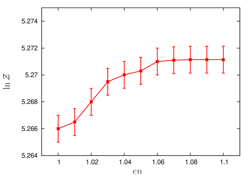
with $\mathbf{x}_{\rm i}$ denoting the vectors of the active point set. This ensures that all active points are enclosed within the ellipse although there does, of course, still exist the possibility that some parts of the region $\mathcal{L}>\mathcal{L}_{\rm i}$ lie outside the ellipse and so we still require an enlargement factor but one that is generally smaller than that required by Mukherjee’s method. In Fig 2 evidence estimates are shown calculated with a range of enlargement factors $1.0<en<1.1$ as determined for a relatively complex posterior of multiple Gaussians where the analytic $\ln\mathcal{Z}=5.271$. The algorithm succesfully converges to the correct value with an enlargement factor of $\sim 1.06$.

Figure 2: $\ln\mathcal{Z}$ as determined for a range of enlargement factors for a multiple Gaussian posterior, the analytic value in 5.271.

Computationally it is convenient to draw the random samples not from this ellipsoidal bound directly but from a unit sphere centred on the origin. Thus, we construct a transformation matrix $\textbf{{T}}=k\textbf{{X}}^{\textbf{{T}}}\textbf{{D}}^{\prime}$ where $\textbf{{C}}^{\prime}=\textbf{{D}}^{\prime}\textbf{{D}}^{\prime}$ which maps points from the unit sphere into the ellipse (centred at the origin) so a uniform deviate $\mathbf{x}$ drawn from the sphere forms a point within the ellipse $\mathbf{y}$ via

$$\mathbf{y}=\textbf{{T}}\mathbf{x}+\mathbf{c}.$$ (11)

Generating deviates from a uniform $n$-sphere can be most easily achieved by drawing a set of $n$ Gaussian random numbers $\mathbf{z}$ (via the Box-Muller algorithm), scaling to give a point uniformly distributed on the surface of the sphere $\mathbf{z}^{\prime}=\frac{1}{r}\mathbf{z}$ where $r=\sum z_{i}^{2}$ and finally scaling again by a deviate drawn from a quadratic distribution between 0 and 1 to generate a point uniformly within the sphere. It is worth pointing out that the number of active points $N$ must always be greater than the dimensionality of the parameter space in order for the ellipse to be defined unambiguously.

3.2 Recursive Clustering

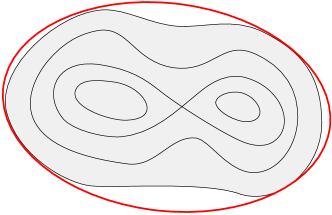
The usefulness of ellipsoidal sampling is reduced for posteriors that are not uni-modal. Our extension allows the formation of multiple ellipsoids centred on individual isolated peaks in the posterior which can greatly reduce the region of prior sampled and thus increases sampling efficiency. The idea is depicted in Fig. 3 in a toy posterior and equivalently in Fig. 4 in $X-\mathcal{L}$ space, where upon identifying distinct clusters they are separated and fit by individual ellipsoids. While this does violate the requirement that $\mathcal{L}(X)$ be a uniquely valued function we are rescued by the linear nature of the evidence. It is valid to consider each cluster individually and sum the contributions provided we correctly assign the prior masses to each distinct region. Since our collection of $N$ active points is distributed evenly across the prior we can safely assume that the number of points within each clustered region is proportional to the prior mass contained therein.

Figure 3: Cartoon of a simple bimodal case. In (a) we see that the ellipsoid represents a good bound to the active region. In (b)-(d), as we nest inward we can see that the acceptance rate will rapidly decrease as the bound steadily worsens. Figure (e) illustrates the solution, we branch and sample each clustered region in turn.

Figure 4: View of clustering in $\mathcal{L}-X$ space.

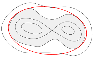
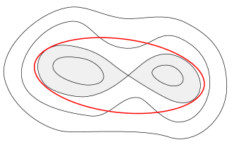
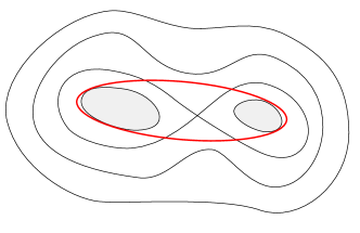
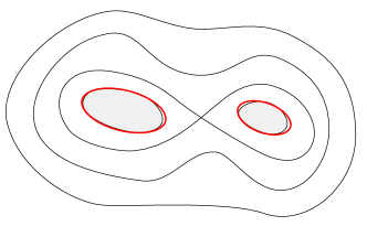
Identifying clusters in the posterior, in the absence of any analytical form for the function, is performed by recursive application of the K-means algorithm with $K=2$. This process is designed to place $N$ data points in an arbitrarily large number of dimensions into $K$ clusters. An iterative process the algorithm starts by dividing the set of samples into two clusters, the mean position of each cluster is then determined and each subsequent point is assigned to one or other of the two mean positions. The next iteration updates the mean positions and so on. In this way a set of sampled data can be searched by the alorithm for clustering centres. For a more detailed discussion of the $K$-means process see for example see MacKay 2003. While our implementation does not require the user to know beforehand any details about the shape of the posterior, the algorithm does contain a number of user definable parameters which can guide the clustering. These parameters define two conditions that must be met once two separate clusters have been identified via K-means. The first is a volume reduction factor set so that the total volume of the combined clustered ellipsoids is less than some fraction of the pre-clustered ellipsoid. The second parameter requires that the clusters are sufficiently separated by some distance to avoid overlapping regions. We have found reasonable values for the former to be $\sim 0.3$ while the latter seperation criteria requires a new ellipse to be at least $1.1$ times the existing ellipse major axis in each dimension. If these conditions are met clustering will occur and the algorithm will search independently within each cluster for further sub-clusters. This process continues recursively until some stopping criterion (discussed in Sec. 3.3.) is met. So long as condition (i) is met we will be guaranteed a performance improvement as less of the prior needs to be sampled at each cycle.

The division of prior mass between two clusters introduces a further source of error, and we can no longer simply assess the uncertainty in $\mathcal{Z}$. To resolve this we must find the probability of the mass fraction in each cluster. If we have a fraction $f_{1}$ in cluster 1, with a total number of points $N$, the probability of $n_{1}$ points in cluster 1 is simply binomial:

$$P(n_{1}|f_{1},N)=\frac{N!}{n_{1}!(N-n_{1})}f_{1}^{n_{1}}(1-f_{1})^{N-n_{1}}$$ (12)

We can invert this using Bayes’ theorem with a uniform prior to yield $P(f_{1}|n_{1},N)$ and draw samples via MCMC which can then be used, as in Sec. 3 to generate a variance for each cluster which can be summed to give the total error.

3.3 Stopping Criterion

We wish to stop the calculation on determining the evidence to some specified accuracy. One way would be to proceed until the evidence estimated at each replacement changes by less than a specified tolerance. However, this could for example underestimate the evidence in cases where the posterior contains any narrow peaks close to its maximum. Skilling (2004) provides an adequate and robust condition by determining an upper limit on the evidence that could be determined from the remaining set of current active points.

By selecting the maximum likelihood $\mathcal{L}_{\text{max}}$ in the set of active points one can then safely assume that the largest evidence contribution that can be made by the remaining portion of the posterior is $\Delta{\mathcal{Z}}_{\rm i}=\mathcal{L}_{\rm max}X_{\rm i}$ i.e. the product of the remaining prior mass and maximum likelihood. We choose to stop when this quantity would no longer change the final evidence estimate by some user defined factor.

4 Applications

To demonstrate the capabilities of clustered nested sampling we now take three specific examples; the first two involve posteriors of known functional form so that an analytic evidence can be compared with that found through our nested sampling algorithm and the final example demonstrates a cosmological application involving a bi-modal posterior.

4.1 Toy model I

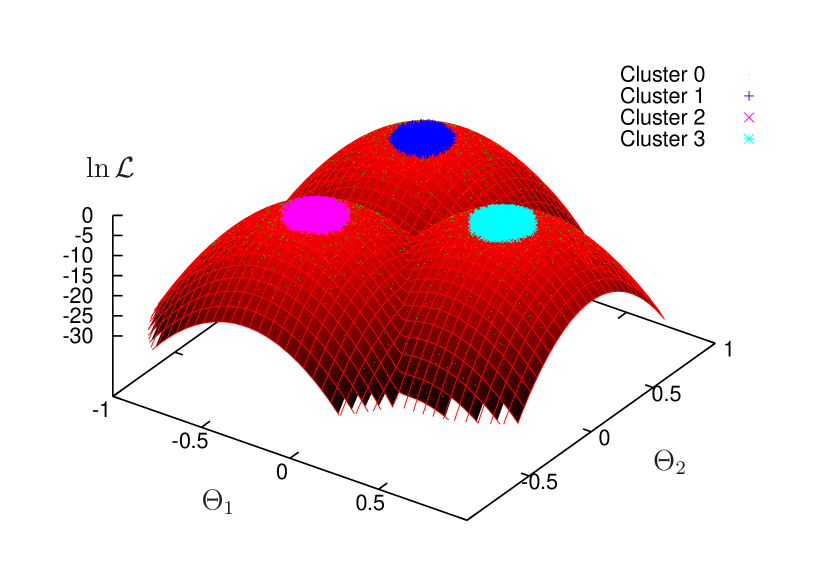
Our first example posterior consists of 3-Gaussian peaks in a two dimensional parameter space. The clustering (see Fig. 5) algorithm first divides the space into cluster 1 and cluster 2+3, runs to the required accuracy on cluster 1 then returns to the combination of clusters 2+3, immediately clusters to separate 2+3 then running both successively to completion. Table 1 shows that with and without clustering we can determine the evidence to within 2 % of the analytic value. To obtain similar accuracy, however the clustered example required only 5 % of the number of likelihood evaluations. Our calculated errors agree to within 10 % of the sampling errors based on 50 repetitions.

Figure 5: Toy Model I: Posterior consisting of 3 Gaussian peaks placed at the vertices of an equilateral triangle in the x-y plane at a distance of 0.5 units from the origin with $\sigma=0.1$. The clusters found are depicted in colour at each peak.

Table 1: Summary of sampling statistics with and without clustering for the 3-Gaussian posterior with a log-evidence, determined analytically of 2.813.

Toy Model I:	Clustering	No Clustering
$\ln{\mathcal{Z}}$	2.798	2.830
$N_{\rm like}$	12,115	258,361
Sampling Error	0.063	0.060
Calculated Error	0.061	0.059

4.2 Toy model II

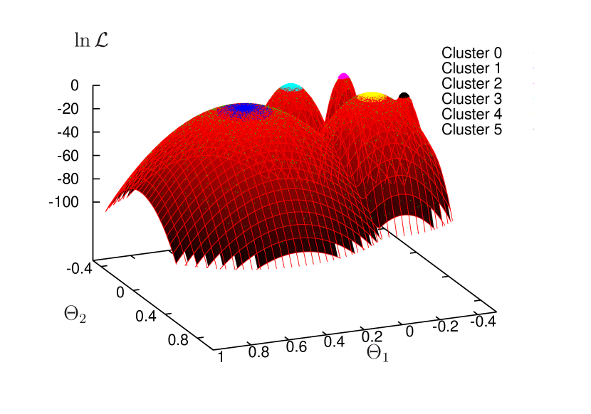
Posteriors that occur in typical applications may be far more complicated than that used in Sec. 4.1. Our second example uses a combination of five Gaussians of varying width and height in the x-y plane (see Fig. 6). Clustering occurs naturally in the expected fashion, producing a improvement in efficiency of at least a factor of 3 (see Table 2). Note in particular the algorithm correctly isolates the slim Gaussian in cluster 5 superimposed on the larger Gaussian at cluster 4.

Figure 6: Toy Model II: Posterior consisting of 5 Gaussian peaks spaced randomly in the x-y plane of varying width and height. The clusters found are depicted in colour at each peak.

Table 2: Summary of sampling statistics with and without clustering for the multi-Gaussian posterior with a log-evidence determined analytically of 5.271.

Toy Model II:	Clustering	No Clustering
$\ln{\mathcal{Z}}$	5.296	5.230
$N_{\rm like}$	1,016,994	3,615,300
Sampling Error	0.083	0.085
Calculated Error	0.084	0.084

4.3 Cosmological application

Recent measurements of the Cosmic Microwave Background (CMB) by WMAP indicate a deficiency of power on large scales when compared with a flat $\Lambda{\rm CDM}$ cosmological model. One possibility is that this decrease is caused by a feature in the primordial spectrum of density perturbations, specifically a sharp cutoff on scales $k\leq 0.0003$ Mpc^-1. Many analyses to date have examined various forms for this cutoff (for example Efstathiou 2003; Bridle et al. 2003; Shafieloo & Souradeep 2003; Lasenby & Doran 2005), here we will examine a model with favourable likelihood as determined by Sinha & Souradeep (2006) using WMAP 1-year TT data (Bennett et al., 2003). The posterior derived for this model/data combination contains substantial multi-modality in the parameters defining the spectrum.

Physically a sharp cutoff can be generated by a kink in the inflationary potential (Starobinsky, 1992), followed by a ‘bump’ and damped oscillations at larger $k$. This effect can be modelled via a transfer function applied to any underlying spectrum $P(k)=P_{0}(k)T^{2}(y,R_{\ast})$ where $y=k/k_{\ast}$ and

$$T^{2}(y,R_{\ast})=1-3(R_{\ast}-1)\frac{1}{y}\left[\left(1-\frac{1}{y^{2}}\right)\sin 2y+\frac{2}{y}\cos 2y\right]\\ +\frac{9}{2}(R_{\ast})^{2}\frac{1}{y^{2}}\left(1+\frac{1}{y^{2}}\right)\\ \left[1+\frac{1}{y^{2}}+\left(1-\frac{1}{y^{2}}\right)\cos 2y-\frac{2}{y}\sin 2y\right].$$ (13)

$R_{\ast}$ is the ratio of inflationary potential and scalar field where $k_{\ast}$ is the cutoff wave-vector. The best fit model as found by Sinha & Souradeep (2006) was a slight variant on this with an exponential cutoff such that the underlying spectrum is a single index spectrum with exponential decay, governed by a factor $\alpha$:

$$P(k)=A(1-e^{(0.75y)^{\alpha}})k^{n-1}T^{2}.$$ (14)

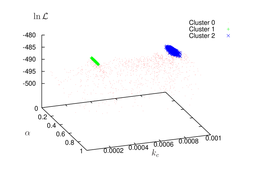
We have restricted the analysis to the set of parameters defining the spectrum only ($n_{s}$, $k_{c}$, $\alpha$, $R_{\ast}$, $A_{s}$) and fixed the remaining parameters to their best fit values as determined via MCMC using the CosmoMC package (Lewis & Bridle, 2002) (namely $\Omega_{b}h^{2}=0.0243$, $\Omega_{c}h^{2}$ = 0.115, $\theta=1.04$ and $\tau=0.22$). The results of Starobinsky (1992) suggest that the posterior is bimodal in the subspace $(\alpha,k_{c})$, andso this problem provides an ideal example of the applicability of clustering. The algorithm correctly identifies both peaks and clusters accordingly (see Fig. 7). The marginalised posteriors for each parameter are shown in Fig. 8

The maximum likelihood point in the marginalised posterior of $k_{c}$ is clearly centred at $0.0003$ Mpc^-1 (see Fig. 8) with a secondary peak also visible at approximately $0.0006$ Mpc^-1. These features provide an ideal example of the applicability of clustering. The algorithm correctly identifies both peaks and clusters accordingly (see Fig. 7).

Figure 7: Cosmological Application: Set of replacement samples in the cutoff scale $k_{c}$ and $\alpha$ with clustered regions shown.

Figure 8: Cosmological Application: 1-D marginalised posteriors for model spectral parameters, comparing those obtained via MCMC (red) and nested sampling (black).

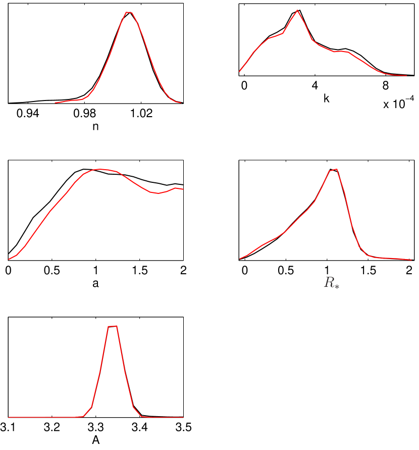
We completed 10 separate evaluations of the evidence via the three most common methods for comparison. Table 3 summarises the evidences obtained, their associated errors in sampling (i.e. the standard error over the 10 runs), the calculated error estimated via the method described in Sec. 3.3 and the number of likelihood calls made per individual run. Both nested sampling methods provide significant improvements in $N_{\rm like}$ over thermodynamic integration . With clustering however we see a further performance increase by more than a factor of 2 for similar statistical uncertainties. Moreover, the sampling error and our calculated error show extremely good agreement, eliminating the need to perform more than one evidence calculation and thus further reducing the computational cost by an order of magnitude.

Table 3: Sampling statistics for the Starobinsky model via nested sampling (both clustered and without) and thermodynamic integration (TI).

Example III:	Clustering	No Clustering	TI
$\ln{\mathcal{Z}}$	494.65	494.45	493.76
$N_{\rm like}$	96,720	250,523	$>$ 400,000
Sampling Error	0.29	0.31	0.87
Calculated Error	0.30	0.29	–

5 Conclusions

We have demonstrated the applicability of our clustered nested sampling algorithm to multi-modal posterior distributions in both simulated ‘toy’ models and a cosmological example based on the Starobinsky primordial power spectrum –in which a substantial performance increase was noted. Although we have examined here a multi-modal cosmological example, our sampler is by no means restricted to such use. In fact we feel an important feature is the ability to determine the variance of the final evidence value, for any model, without calculating the sample variance over repetitive runs. This alone reduces the computational load by at least an order when compared with previous methods.

References

- Basset et al. (2004) Basset B.A., Corasaniti P.S., Kunz, M., Astrophys. J. Lett., 2004, 617, L1
- Beltran et al. (2005) Beltran M., Garcia-Bellido J., Lesgourgues J., Liddle A., Slosar A., 2005, Phys. Rev. D, 71, 063532
- Bennett et al. (2003) Bennett C.L., et al., 2003, ApJS, 148, 1
- Bridges et al. (2006) Bridges M., Lasenby A.N., Hobson, M.P., 2006, MNRAS, 369, 1123
- Bridle et al. (2003) Bridle S., Lewis A., Weller J., Efstathiou G., 2003, MNRAS, 342, L72
- Efstathiou (2003) Efstathiou G., 2003, MNRAS, 343 L95
- Hobson et al. (2003) Hobson M.P., Bridle S.L., Lahav O., 2002, MNRAS, 335, 377
- Jeffreys (1961) Jeffreys H., 1961, Theory of Probability, 3rd ed., Oxford University Press, Oxford
- Lasenby & Doran (2005) Lasenby A.N., Doran, C., 2005, Phys.Rev. D 71, 063502
- Lewis & Bridle (2002) Lewis A. and Bridle S., 2002, Phys. Rev. D, 66, 103511
- MacKay (2003) MacKay D.J.C., 2003, Information Theory, Inference and Learning Algorithms. Cambridge University Press, Cambridge
- Mukherjee et al. (2006) Mukherjee P., Parkinson D., Liddle A.R., 2006, ApJ, 638, L51
- Niarchou et al. (2004) Niarchou A., Jaffe A., Pogosian L., 2004, Phys.Rev. D 69 063515
- Sinha & Souradeep (2006) Sinha R., Souradeep T., 2006, Phys.Rev. D74 043518
- Skilling (2004) Skilling J., 2004, ‘Nested Sampling for General Bayesian Computation’, http://www.inference.phy.cam.ac.uk/bayesys
- Slosar et al. (2003) Slosar A. et al., 2003, MNRAS, 341, L29
- Shafieloo & Souradeep (2003) Shafieloo, A., Souradeep, T., 2004, Phys. Rev. D, 70, 043523
- Starobinsky (1992) Starobinsky A.A., 1992, JETP Lett, 55, 489
- Trotta (2005) Trotta, R. 2007, MNRAS, 378, 72