2003–2005 INTEGRAL and XMM-Newton observations of 3C 273

Abstract

Aims. The aim of this paper is to study the evolution of the broadband spectrum of one of the brightest and nearest quasars 3C 273.

Methods. We analyze the data obtained during quasi-simultaneous INTEGRAL and XMM-Newton monitoring of the blazar 3C 273 in 2003–2005 in the UV, X-ray and soft $\gamma$-ray bands and study the results in the context of the long-term evolution of the source.

Results. The 0.2-100 keV spectrum of the source is well fitted by a combination of a soft cut-off power law and a hard power law. No improvement of the fit is achieved if one replaces the soft cut-off power law by either a blackbody, or a disk reflection model. During the observation period the source has reached the historically softest state in the hard X-ray domain with a photon index $\Gamma=1.82\pm 0.01$. Comparing our data with available archived X-ray data from previous years, we find a secular evolution of the source toward softer X-ray emission (the photon index has increased by $\Delta\Gamma\simeq 0.3-0.4$ over the last thirty years). We argue that existing theoretical models have to be significantly modified to account for the observed spectral evolution of the source.

1 Introduction

3C 273 is a radio loud quasar, with a jet showing superluminal motion, discovered at the very beginning of quasar research. Being one of the brightest and nearest (z=0.158) quasars, 3C 273 was intensively studied at different wavelengths (see Courvoisier (1998) for a review).

In the X-ray band 3C 273 is thought to be quite a unique source in the sense that in its X-ray spectrum the “blazar-like” emission from the pc-scale jet mixes with the “nuclear” component, which reveals itself through the presence of a large blue-bump and a so-called “soft excess” below $\sim 1$ keV. Both are typical for emission from the nuclei of Seyfert galaxies. During the observation period discussed in this paper the radio to millimeter component, usually associated with a jet, has been in its lowest state. Thus, our data provide an opportunity to study the “nuclear” component in more details and to test theoretical models for the emission of 3C 273.

Surprisingly, in spite of the low level of the “jet-like” contribution, our data do not reveal the presence of typical “Seyfert-like” features in the spectrum. In fact, the 0.2-100 keV spectrum is well fitted by a simple model composed of two power laws or a combination of a hard power law with a soft cut-off power law. We find that more sophisticated models, which include a black-body for description of the soft excess, or a disk reflection component give comparable or worse fits to the data, than the above simple model. Moreover, the “disentanglement” of Seyfert and jet components of the X-ray spectrum, as proposed by Grandi & Palumbo (2004), is not observed in our data set.

Walter & Courvoisier (1992) have found an anticorrelation between the X-ray spectral slope and the ratio of X-ray to ultraviolet (UV) luminosity of 3C 273 using quasi-simultaneous data from EXOSAT, GINGA and IUE obtained in the 80-s. They have interpreted this correlation as evidence that the X-ray emission is due to thermal Comptonization of the UV flux. The presence of optical monitors on-board of both XMM-Newton  and INTEGRAL enables us to analyze correlations between the big blue bump variability and the variability in X-rays. Repeating the analysis of Walter & Courvoisier (1992) with our data set we do not find the previously observed X-ray slope – UV/X-ray flux correlation. The disappearance of this correlation is even more surprising because of the appearance of a previously unobserved correlation between the UV and the X-ray flux from the system. Taking into account the fact that the typical variability time scales in the UV and the X-ray bands are different (months in UV and days in X-ray), true simultaneity of the observations could be important. Our XMM-Newton and INTEGRAL observations are the first observations in which UV and X-ray data were taken at the same time.

It is possible, however, that appearance/disappearance of the UV–X-ray correlation reflects a real evolution of the spectral state of the source during the last 30 years. Collecting the archival X-ray data for about 30 years of observations, we find that the source indeed evolves towards a softer X-ray state. We find that the source has reached its historically softest X-ray state with photon index $\Gamma=1.82\pm 0.01$ in June 2003. This spectral slope is (by $\Delta\Gamma\simeq 0.3-0.4$) softer than the typical slope observed in the 70-s and 80-s. This is definitely larger than the typical short time scale fluctuations of the slope which are at a level of $\Delta\Gamma\simeq 0.1$.

It is important to note that spectral evolution of the source should not be ignored in theoretical modelling of nuclear and jet emission from 3C 273. For example, the very hard spectral state of the source in the late 70-s has led Lightman & Zdziarski (1987) to the conclusion that “compact source” type models dominated by pair production can not be applied to 3C 273 in spite of its high apparent compactness. However, this conclusion is not applicable for the present state of the source. Similarly, the most popular model for the hard X-ray spectrum of the source, inverse Compton emission from the pc-scale jet, is satisfactory for the present state of the source, but cannot explain the $\Gamma\simeq 1.4$ spectral index observed in 70-s.

The paper is organized as follows: in Section 2 we present the sequences of observations and methods used for data reduction and analysis. In section 3 we present the results obtained, and discuss them in Section 4. We then give a summary of our analysis in the last part of the paper.

2 Observations and Data Analysis

2.1 INTEGRAL observations

Since the launch of INTEGRAL (Winkler et al., 2003) on October 17, 2002, 3C 273 was regularly monitored. Details of the data used in the current analysis are given in Table 1. The preliminary analysis of the 2003 data was done by Courvoisier et al. (2003a). A detailed study of the multiwavelength spectrum of June 2004 was presented by Türler et al. (2006).

Table 1: INTEGRAL observations of 3C 273.

Period	Tstart	Rev	On Time	ISGRI/SPI/JEM-X
			(ks)	Exposure(ks)
1a	2003-01-05	28	120.8
1b	2003-01-11	30	10.6
1c	2003-01-17	32	106.8
1				182.5/182.4/12.4
2a	2003-06-01	77	57.0
2b	2003-06-04	78	52.6
2c	2003-06-16	82	33.5
2e	2003-07-06	89 – 90	227.1
2f	2003-07-18	93	20.5
2g	2003-07-23	94	14.0
2				308.9/310.5/40.3
3	2004-01-01	148 – 149	26.4	152.3/NA/13.8
4	2004-06-23	207	92.7	67.1/NA/29.2
5a	2005-05-28	320 – 321	278.3
5b	2005-07-09	334	102.5
5				269.1/367.2/68.7

During the INTEGRAL observations 3C 273 was all the time in a very low state, with a flux of several milliCrabs (see Section 3.2). To obtain better statistics for spectral analysis we have combined data taken within a few weeks, which resulted in five data sets. The combined exposure times for each data set and each instrument on-board of INTEGRAL are listed in Table 1.

The data for all INTEGRAL instruments were analysed in a standard way with the latest version of the off-line scientific analysis (OSA) package 5.1 distributed by ISDC (Courvoisier et al., 2003b).

Most of the time, observations were done in the $5\times 5$ dithering mode. The staring mode was used only during revolutions 30, 148, and 149. It is therefore not possible to use SPI data during the third period. There are also no SPI data during the fourth period, as the instrument was in the annealing mode during this observation.

For the analysis of the INTEGRAL/JEM-X observations we have selected science windows for which the source was less than 3.5^∘ from the center of the field of view. During the first three periods JEM-X 2 was operating, while during the fourth and fifth period it was switched off, and data were taken with the JEM-X 1 telescope.

To minimize the influence of the flares in the surrounding background of the charged particles we have not used pointings in which the detector countrate exceeds the mean of the given period by more than 5%.

2.2 XMM-Newton observations

The log of the XMM-Newton observations analyzed in this paper is presented in Table 2. Among all the observations of the source done with XMM-Newton we have selected those that were done while INTEGRAL was observing.

Table 2: XMM-Newton observations of 3C 273.

Period	Date	Revolution	On Time	PN Exposure Time
			(ks)	(ks)
1	2003-01-06	563	8.95	5.97
2	2003-07-07	655	58.56	40.60
3	2003-12-14	735	8.91	5.77
4	2004-06-30	835	62.91	13.93
5	2005-07-10	1023	28.11	19.33

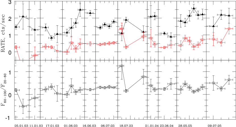
Figure 1: top panel: 2003–2005 IBIS/ISGRI lightcurves of 3C 273in 20-60 keV (upper curve, black) and 60-100 keV (lower curve, red). The data are binned in 1-d intervals. For each time frame the date given at the bottom corresponds to the first data point, tick interval is 1 day. bottom panel: Hardness ratio F${}_{(60-100\,keV)}$/F${}_{(20-60\,keV)}$.

The XMM-Newton Observation Data Files (ODFs) were obtained from the on-line Science Archive. The data were processed and the event-lists filtered using xmmselect within the Science Analysis Software (sas), version 6.5 and the most up-to-date calibration files. All EPIC observations were performed in the Small Window Mode. In all observations the source was observed with the MOS1, MOS2 and the PN detectors. As the PN detector, in contrast to MOS1 and MOS2, is not affected by pile-up in our observations we concentrate our analysis on the PN data only. Patterns 0-4 were used in the analysis. Background spectra were extracted from areas of the sky close to 3C 273 showing no obvious sources. ARFGEN and RMFGEN were then run to produce the corresponding ARF and RMF files.

Optical and ultraviolet fluxes were obtained with the optical monitor (OM) of XMM-Newton with omichain following the instructions of the SAS Watchout page and using the values provided for an AGN spectral type. The resulting magnitudes are given in Table 3. No OM data for the selected filters are available for Period 3.

Table 3: Optical and UV magnitudes of 3C 273 during each observational period.

	Period 1	Period 2	Period 4	Period 5
V		12.53$\pm$0.01	12.69$\pm$0.01	12.57$\pm$0.01
B			12.95$\pm$0.01	12.86$\pm$0.01
U		11.62$\pm$0.01	11.76$\pm$0.01	11.69$\pm$0.01
UVW1	11.32$\pm$0.01	11.28$\pm$0.01	11.44$\pm$0.01	11.30$\pm$0.01
UVM2	11.34$\pm$0.01		11.37$\pm$0.01	11.19$\pm$0.01
UVW2		11.14$\pm$0.01	11.36$\pm$0.01	11.16$\pm$0.01

3 Results

3.1 Timing Analysis

In the top panel of Figure 1 we show the 3C 273 IBIS/ISGRI lightcurves in the 20-60 keV (black points) and in the 60-100 keV (red points) energy ranges. In this figure the data are binned in one day intervals. ISGRI data show that the hard X-ray emission from the system is variable on at least a one day time scale. In order to investigate the nature of this variability we have produced the “flux-flux” diagram for the 20-60 keV and 60-100 keV energy bands, shown in the bottom right panel of Fig. 8. Large error bars of the single-day flux measurements do not allow to see the general trend of the dependence between the 20-60 keV and 60-100 keV flux. However, rebinning the data by building the average of three adjacent (along the 20-60 keV flux axis) original data points in the flux-flux plot we find that the whole data set has a roughly linear behaviour (Spearman correlation coefficient is equal to $R=0.89$, with a probability of random coincidence $P_{rand}=7\times 10^{-3}$). This indicates that the variability of the source in the 20-100 keV band is mostly due to changes in the normalization, but not in the shape of the spectrum.

Fig. 2 shows the XMM-Newton lightcurves in 0.2–1 keV (upper curve, black) and 3–10 keV (lower curve, red) bands. One can see significant changes of the 0.2–1 keV flux from data set to data set, but the variability at the time scale of single observation, $\sim 10$ ksec is negligible. The plot of the hardness ratio (bottom panel of Fig. 2) shows that the 0.2-10 keV spectrum hardens toward the end of the observation period.

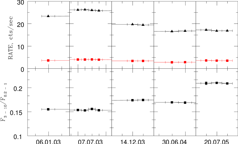
Figure 2: top panel: 2003–2005 XMM/PN lightcurves of 3C 273in 0.2–1 keV (upper curve, black) and 3–10 keV (lower curve, red). The data are binned in quarter of day intervals. bottom panel: Hardness ratio F${}_{(3-10\,keV)}$/F${}_{(0.2-1\,keV)}$.

3.2 Spectral Analysis

Our INTEGRAL and XMM-Newton observations provide a very broad band (5 decades in energy) set of quasi-simultaneous data which spans from the UV ($\sim 1$ eV) up to the soft gamma-ray ($\sim 100$ keV) band. The spectra of the source for all the five selected data sets are shown in Fig. 3. Taking into account a wide range of theoretical models proposed for the X-ray spectrum of 3C 273 we adopt a “simple to complex” strategy in the spectral analysis and attempt first to find a “minimal model” which can provide a satisfactory representation of the data and then consider how changing and/or adding various theoretically motivated components improves or worsens the fit. The hydrogen column density was fixed to the galactic value $N_{H}=1.79\times 10^{20}cm^{-2}$ (Dickey & Lockman, 1990).

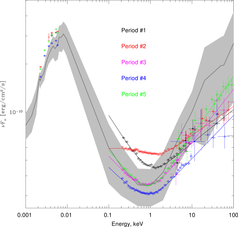
Figure 3: Broadband spectra of 3C 273 for each period. Data are fitted with the simple phenomenological model described in Table 5. The new data are compared to the average flux (grey line) and the 1-$\sigma$ variability range (grey area) based on historic data of 3C 273 (Türler et al., 1999).

3.2.1 Phenomenological model

Data in the 2–100 keV energy range are well fitted by a simple power law, see Table 4. In our analysis we have left the ISGRI, SPI and JEM-X intercalibration factors free to vary with respect to the PN camera. The significant variation of the JEM-X intercalibration factor reflects a known change of the gain parameters of the instrument. It is possible to fit all the data with the same SPI ($C_{s}=1.41)$ and ISGRI ($C_{i}=1.19$) intercalibration factors, but we have preferred not to do this, as the XMM-Newton and INTEGRAL data are only quasi-simultaneous, and the different value of the flux measured by XMM-Newton and INTEGRAL can be due to the physical change of the source flux on a one month scale. The fit of the second data set can be improved by the addition of a broad emission line as discussed below.

Table 4: Parameters of the single power-law model in 2-100 keV energy range. The fit was done leaving free intercalibration factors for ISGRI (C_i), SPI (C_s) and JEM-X (C_j) with respect to the PN camera. The parameter uncertainties correspond to 1 $\sigma$ level.

	Period 1	Period 2	Period 3	Period 4	Period 5
Power law
$\Gamma$	$1.81^{+0.01}_{-0.01}$	$1.84^{+0.01}_{-0.01}$	$1.70^{+0.01}_{-0.01}$	$1.75^{+0.01}_{-0.01}$	$1.66^{+0.01}_{-0.01}$
$F_{2-10}^{*}$	$8.79^{+0.17}_{-0.16}$	$10.10^{+0.04}_{-0.07}$	$8.04^{+0.13}_{-0.12}$	$6.72^{+0.10}_{-0.09}$	$8.54^{+0.09}_{-0.09}$
Intercalibration factors
$C_{j}$	$1.11^{+0.09}_{-0.09}$	$1.35^{+0.05}_{-0.05}$	$1.33^{+0.09}_{-0.09}$	$0.30^{+0.11}_{-0.11}$	$0.67^{+0.05}_{-0.05}$
$C_{i}$	$0.92^{+0.05}_{-0.05}$	$1.22^{+0.03}_{-0.03}$	$1.42^{+0.11}_{-0.11}$	$0.98^{+0.08}_{-0.07}$	$1.23^{+0.04}_{-0.04}$
$C_{s}$	$1.39^{+0.26}_{-0.25}$	$1.49^{+0.16}_{-0.16}$	–	–	$1.67^{+0.15}_{-0.14}$
Statistics
$\chi^{2}$	920	1673	950	1139	1419
(dof)	(920)	(1632)	(1153)	(1205)	(1390)

^⋆ In units of $10^{-11}$ erg cm^-2 s^-1.

Figure 4: A 3C 273 spectrum in the 4-7 keV energy band as observed with XMM/PN in July 2003 (second data set). Data are fitted with a single power law. A broad iron line is marginally visible in the residuals (see text).

The simplest satisfactory fit to the 0.2-100 keV data can be achieved with a model consisting of two power laws. A soft power law with a photon index $\Gamma_{1}$ dominates in the energy band below 2 keV and describes the so-called ”soft excess”. A hard power law with photon index $\Gamma_{2}$ dominates in the hard X-ray band. An F-test shows that a slightly better fit to the data can be achieved if one uses a cut-off power law instead of the single power law for the description of the soft emission.

Surprisingly, we find that already this simple model provides a very good fit to the combined INTEGRAL and XMM-Newton data in all the observations except the second one. In the second data set the addition of a broad redshifted emission line at $E_{Fe}=6.65\pm 0.07$ keV in the rest frame of the object makes the fit acceptable. This line can be identified with a fluorescent K_α iron line. A broad iron line was seen in previous observations of 3C 273 by different instruments, see e.g. Yaqoob & Serlemitsos (2000). The large width and marginal detection of the line (see Figure 4) do not allow us to firmly distinguish ionised and non-ionised iron. In all other spectra the addition of an iron line does not significantly improve the fit. For completeness we show the degradation of the fit if no line is included. The complete list of the fit parameters for our phenomenological model is given in Table 5.

Table 5: Parameters of the phenomenological model fit to the data. When the uncertainties are not quoted, the value of the parameter was fixed.

	Period 1	Period 2	Period 3	Period 4	Period 5
Cut-off power law describing Soft excess
$\Gamma_{1}$	$2.46^{+0.14}_{-0.16}$	$2.02^{+0.08}_{-0.08}$	2.37${}^{+0.12}_{-0.13}$	$2.36^{+0.12}_{-0.13}$	$2.32^{+0.10}_{-0.11}$
$E_{1}$	$0.65^{+0.20}_{-0.14}$	$0.52^{+0.06}_{-0.05}$	0.73${}^{+0.24}_{-0.15}$	$0.65^{+0.16}_{-0.12}$	$0.58^{+0.10}_{-0.08}$
$F^{\star}_{0.2-1}$	3.60${}^{+1.08}_{-0.76}$	$2.11^{+0.16}_{-0.26}$	2.34${}^{+0.59}_{-0.41}$	1.89${}^{+0.49}_{-0.35}$	$2.36^{+0.24}_{-0.39}$
Second power law describing hard tail
$\Gamma_{2}$	1.79${}^{+0.02}_{-0.02}$	$1.82^{+0.01}_{-0.01}$	$1.67^{+0.02}_{-0.01}$	$1.73^{+0.01}_{-0.01}$	$1.63^{+0.01}_{-0.01}$
$F_{2-10}^{\star}$	8.76${}^{+0.19}_{-0.21}$	$10.03^{+0.06}_{-0.10}$	8.02${}^{+0.22}_{-0.17}$	$6.70^{+0.10}_{-0.12}$	$8.53^{+0.08}_{-0.10}$
Gaussian line
EFe	6.65	6.65${}^{+0.07}_{-0.07}$	6.65	6.65	6.65
$\sigma_{Fe}$	1.98${}^{+0.55}_{-0.39}$	0.31${}^{+0.07}_{-0.06}$	0.39${}^{+0.22}_{-0.12}$	0.50${}^{+0.92}_{-0.50}$	2.35${}^{+2.97}_{-1.30}$
I${}_{Fe}^{\star\star}$	42.50${}^{+32.32}_{-12.80}$	6.1${}^{+1.3}_{-1.4}$	5.29${}^{+3.31}_{-2.51}$	$3.14^{+3.91}_{-2.79}$	17.14${}^{+5.83}_{-12.31}$
Intercalibration factors
Cj	1.11${}^{+0.09}_{-0.09}$	$1.33^{+0.05}_{-0.05}$	1.31${}^{+0.09}_{-0.09}$	0.37${}^{+0.10}_{-0.10}$	0.66${}^{+0.05}_{-0.05}$
Ci	0.87${}^{+0.05}_{-0.05}$	$1.16^{+0.03}_{-0.03}$	1.38${}^{+0.11}_{-0.10}$	0.97${}^{+0.07}_{-0.07}$	1.19${}^{+0.37}_{-0.35}$
Cs	1.32${}^{+0.24}_{-0.24}$	$1.43^{+0.15}_{-0.15}$	–	–	1.62${}^{+0.14}_{-0.13}$
Statistics
$\chi^{2}$	1305	2174	1360	1594	1832
(df)	(1308)	(2022)	(1519)	(1634)	(1778)
Statistics without iron line taken into account
$\chi^{2}_{nl}$	1316	2204	1364	1596	1836
(df)	(1310)	(2025)	(1521)	(1636)	(1780)

^⋆ in $10^{-11}$ erg cm^-2 s^-1 units.

^⋆⋆⋆ in $10^{-5}$ photons cm^-2 s^-1 units.

3.2.2 Modelling of the soft excess

The “soft excess” below 1 keV is typical of Seyfert galaxies. Several competing models for the physical origin of this component are available. In particular, the most simple “phenomenological” models of the soft excess include a (multi-temperature) black body component. However, the origin of such blackbody component is not clear, because the inferred temperature is usually too high to be accounted for standard accretion disks. More complicated models include e.g. reflection of external X-ray emission from the disk. Attempts to fit the soft excess in our XMM-Newton data with different models give the following results.

Table 6: Parameters of the model which includes a black body to describe the soft excess.

	Period 1	Period2	Period 3	Period 4	Period 5
Black body
T(eV)	$78.9^{+1.5}_{-1.6}$	$87.2^{+0.8}_{-0.7}$	$79.0^{+1.8}_{-1.2}$	$78.0^{+2.0}_{-1.2}$	$82.0^{+1.0}_{-1.0}$
$F_{0.2-1}^{*}$	$1.93^{+0.05}_{-0.06}$	$1.08^{+0.01}_{-0.01}$	$1.21^{+0.03}_{-0.03}$	$0.94^{+0.02}_{-0.03}$	$1.42^{+0.02}_{-0.03}$
Power law
$\Gamma$	$1.892^{+0.007}_{-0.006}$	$1.877^{+0.001}_{-0.001}$	$1.787^{+0.005}_{-0.006}$	$1.815^{+0.005}_{-0.006}$	$1.719^{+0.004}_{-0.003}$
$F_{2-10}^{*}$	$8.48^{+0.05}_{-0.04}$	$9.88^{+0.01}_{-0.01}$	$7.75^{+0.03}_{-0.04}$	$6.52^{+0.02}_{-0.03}$	$8.32^{+0.03}_{-0.02}$
Gaussian line
$E_{Fe}$	$6.65$	$6.72^{+0.04}_{-0.06}$	$6.65$	$6.65$	$6.65$
$\sigma_{Fe}$	$0.10$	$0.10$	$0.10$	$0.10$	$0.10$
$n_{Fe}^{**}$	$4.56^{+1.64}_{-1.57}$	$4.89^{+0.37}_{-1.10}$	$3.54^{+1.29}_{-1.26}$	$2.49^{+0.94}_{-0.95}$	$2.35^{+0.90}_{-0.85}$
Intercalibration factors
$C_{j}$	$1.18^{+0.10}_{-0.10}$	$1.39^{+0.05}_{-0.05}$	$1.41^{+0.10}_{-0.10}$	$0.40^{+0.12}_{-0.11}$	$0.70^{+0.06}_{-0.06}$
$C_{i}$	$1.13^{+0.06}_{-0.05}$	$1.34^{+0.03}_{-0.03}$	$1.80^{+0.12}_{-0.13}$	$1.21^{+0.08}_{-0.08}$	$1.46^{+0.04}_{-0.03}$
$C_{s}$	$1.72^{+0.31}_{-0.31}$	$1.65^{+0.18}_{-0.18}$	–	–	$1.98^{+0.17}_{-0.17}$
Statistics
$\chi^{2}$	1445	2659	1543	1799	2161
(dof)	(1310)	(2024)	(1515)	(1630)	(1780)
Statistics without iron line taken into account
$\chi^{2}_{nl}$	1453	2710	1551	1807	2169
(dof)	(1311)	(2026)	(1516)	(1631)	(1781)

^⋆ In units of $10^{-11}$erg cm^-2 s^-1.

^⋆⋆ In units of $10^{-5}$ photons keV^-1 cm^-2 s^-1.

A black body model for the soft excess does not provide an acceptable fit to the data. Best fit parameters for this model are listed in Table 6.The disk reflection component calculated using the kdblur and reflion models of XSPEC (Ross & Fabian, 2005; Crummy et al., 2006) provides a better description of the soft excess, than the blackbody model. Among the parameters of the reflion model we fit only the spectral slope of the power law emission of the central source, fluxes of the direct and reflected components, and the ionization parameter of the gas $\xi$ ($\xi=4\pi F/n_{H}$, where $F$ is the illuminating energy flux, and $n_{H}$ is the hydrogen number density in the illuminated layer; in the reflion model $\xi$ is restricted to $1<\xi<10000$ erg cm s^-1). Parameters of the model fit are given in Table 7. In this Table we also report the measured ratio $R$ of the reflected flux to the total flux expressed in percents.

Table 7: Parameters of the model consisting of emission from the central source reflected from the relativistically-blurred photoionized disc and a jet

	Period 1	Period 2	Period 3	Period 4	Period 5
Direct and reflected emission from the central source
$\xi^{+}$	$2977^{+1565}_{-1126}$	$10000^{+0}_{-248}$	$3170^{+3360}_{-1433}$	$10000^{+0}_{-2453}$	$2570^{+2391}_{-410}$
$F_{0.2-1}^{*}$	$5.78^{+0.71}_{-0.72}$	$4.31^{+0.31}_{-0.36}$	$4.59^{+0.60}_{-0.59}$	$4.05^{+0.63}_{-0.39}$	$3.88^{+0.16}_{-0.35}$
$\Gamma_{1}$	$2.83^{+0.07}_{-0.08}$	$2.56^{+0.01}_{-0.02}$	$2.56^{+0.08}_{-0.08}$	$2.48^{+0.07}_{-0.09}$	$2.76^{+0.04}_{-0.01}$
$R$(%)	$2.39^{+3.98}_{-1.00}$	$20.02^{+179.51}_{-2.39}$	$2.61^{+2.01}_{-1.56}$	$11.38^{+10.69}_{-7.11}$	$2.69^{+3.41}_{-1.15}$
Power law describing Jet emission
$\Gamma_{2}$	$1.70^{+0.03}_{-0.02}$	$1.75^{+0.01}_{-0.02}$	$1.53^{+0.04}_{-0.03}$	$1.55^{+0.05}_{-0.06}$	$1.54^{+0.03}_{-0.02}$
$F_{2-10}^{*}$	$8.05^{+0.27}_{-0.57}$	$9.23^{+0.25}_{-0.36}$	$6.88^{+0.60}_{-0.75}$	$5.76^{+2.63}_{-2.80}$	$8.02^{+2.68}_{-0.38}$
Gaussian line
$E_{Fe}$	$6.65$	$6.73^{+0.05}_{-0.06}$	$6.65$	$6.65$	$6.65$
$n_{Fe}^{**}$	$3.81^{+1.57}_{-1.56}$	$3.06^{+0.62}_{-0.63}$	$2.28^{+1.37}_{-1.35}$	$0.20^{+0.93}_{-0.20}$	$1.42^{+0.94}_{-0.86}$
Intercalibration factors
$C_{j}$	$1.10^{+0.04}_{-0.05}$	$1.19^{+0.02}_{-0.02}$	$1.28^{+0.05}_{-0.54}$	$0.35^{+0.05}_{-0.05}$	$0.66^{+0.04}_{-0.02}$
$C_{i}$	$0.77^{+0.09}_{-0.09}$	$1.17^{+0.04}_{-0.05}$	$1.12^{+0.09}_{-0.09}$	$0.76^{+0.10}_{-0.10}$	$1.08^{+0.05}_{-0.05}$
$C_{s}$	$1.16^{+0.21}_{-0.21}$	$1.30^{+0.14}_{-0.14}$	–	–	$1.35^{+0.12}_{-0.11}$
Statistics
$\chi^{2}$	1399	2239	1349	1516	1819
(dof)	(1410)	(2002)	(1507)	(1542)	(1758)
Statistics without iron line taken into account
$\chi^{2}_{nl}$	1405	2262	1353	1516	1822
(dof)	(1412)	(2004)	(1509)	(1543)	(1759)

⁺ in units of erg cm s^-1.

^⋆ in units of $10^{-11}$ erg cm^-2 s^-1.

^⋆⋆ in units of $10^{-4}$ photons keV^-1 cm^-2 s^-1.

One should note, however, that the amount of reflection found in each data set, except for data set number 2, is at the level of several percent. Thus, a better fit (compared to blackbody) to the data is explained not by the careful account of reflection features, but by a large contribution of the direct power law illuminating the disk, so that the disk reflection model is not significantly different from the previous phenomenological model. To summarize, we find that neither the black body nor the disk reflection provide better descriptions of the soft excess than the (cut-off) power law.

Compton reflection is characterized by a ”reflection hump” at about 30 keV. To look for the presence of a reflection component in the spectrum we have also tried to fit the spectra above 2 keV with either a simple power law or a direct plus reflected power law (the reflion model of XSPEC) and compare the quality of the fits. Although we find that the addition of the reflected component at the level of about 20% improves the quality of the fits, the F-test shows that the probability that this improvement is coincidental is at the level of 10%, so that no definitive conclusion about the presence of a reflection hump in the spectrum can be made. One should note that the largest uncertainty is due to the fact that the ISGRI instrument is sensitive only above $\sim 20$ keV, while XMM-Newton data are available only below $\sim 10$ keV and, in fact, there is a degeneracy between the normalization of the reflection hump and the ISGRI – XMM-Newton intercalibration factor.

A combination of black-body and reflection components, suggested as a best-fit model for the Beppo-SAX data by Grandi & Palumbo (2004) does not change the above conclusion (see below), leaving the (cut-off) power law to be the best model for the soft excess.

Figure 5: The dependance of the 0.2-2 keV black-body emission (left), the 2-10 keV jet like flux (middle), and the iron line flux (right) on the 2-10 keV Seyfert-like flux. Data points are taken from Table 8

3.2.3 Disentangling the Jet and Seyfert contributions

Grandi & Palumbo (2004) (GP) have put forward a strong claim that Seyfert and “jet” components of the X-ray spectrum could be disentangled in the case of 3C 273 so that the observed variations of the X-ray spectral shape are successfully described by variations in the normalizations of the template “jet” and “Seyfert” components. We have tested this hypothesis with our data. For this we repeat the analysis of Grandi & Palumbo (2004). First, we find the “template” models for Seyfert and jet components by fitting simultaneously all the 5 data sets with the same model which consists of a hard power law (jet) and black-body plus partially reflected cut-off power law (Seyfert component). The best fit is achieved with the following parameters: a black body temperature $T_{bb}=75$ eV, a Seyfert component power law slope $\Gamma_{s}=2.25$, a reflection component fraction $RC=0.77$, a jet power law slope $\Gamma_{j}=1.5$, an inclination of the disk $\phi=18^{\circ}$. We assumed solar abundances of elements and fixed the position and width of the iron line at the values found in the second data set: $E_{Fe}=6.65$, $\sigma_{Fe}=0.3$ keV. Then we froze the above parameters and left only the normalizations of the black body, reflection and jet power law components variable. With such a “restricted model” we fit each data set separately and find the normalizations of the three “template” components. The fluxes in each component found in this way are listed in Table 8.

Table 8: Black body, power law, Seyfert-like component and Gaussian line fit to PN, JEM-X, SPI and ISGRI 3C 273 spectra. The fit was done leaving free intercalibration factors for ISGRI (C_i), SPI (C_s) and JEM-X (C_j) with respect to the PN camera. The parameter uncertainties correspond to 1 $\sigma$ level.

	Period 1	Period 2	Period 3	Period 4	Period 5
Black body
$F_{1}^{*}$	$1.01^{+0.05}_{-0.06}$	$<0.004$	$0.53^{+0.03}_{-0.03}$	$0.33^{+0.02}_{-0.03}$	$0.79^{+0.03}_{-0.02}$
Power law
$F_{2}^{*}$	$5.25^{+0.09}_{-0.09}$	$6.32^{+0.03}_{-0.03}$	$5.86^{+0.07}_{-0.06}$	$4.76^{+0.04}_{-0.05}$	$6.74^{+0.05}_{-0.04}$
Seyfert component
$F_{s}^{*}$	$3.47^{+0.04}_{-0.04}$	$3.86^{+0.01}_{-0.01}$	$2.10^{+0.03}_{-0.03}$	$1.96^{+0.02}_{-0.02}$	$1.71^{+0.02}_{-0.02}$
Gaussian line
$n_{Fe}^{**}$	$6.45^{+1.82}_{-3.58}$	$3.03^{+0.99}_{-1.06}$	$4.45^{+2.74}_{-1.51}$	$1.78^{+1.15}_{-1.78}$	$2.92^{+1.76}_{-1.08}$
Intercalibration factors
$C_{j}$	$1.09^{+0.09}_{-0.09}$	$1.26^{+0.05}_{-0.05}$	$1.39^{+0.10}_{-0.10}$	$0.28^{+0.11}_{-0.11}$	$0.65^{+0.05}_{-0.05}$
$C_{i}$	$0.68^{+0.03}_{-0.03}$	$0.80^{+0.02}_{-0.02}$	$1.16^{+0.09}_{-0.09}$	$0.74^{+0.05}_{-0.05}$	$1.05^{+0.02}_{-0.02}$
$C_{s}$	$1.01^{+0.18}_{-0.19}$	$0.97^{+0.11}_{-0.11}$	–	–	$1.42^{+0.12}_{-0.12}$
Statistics
$\chi^{2}$	1340	2342	1383	1561	1913
(dof)	(1311)	(2026)	(1531)	(1565)	(1781)
Statistics without iron line taken into account
$\chi^{2}_{nl}$	1345	2350	1389	1562	1918
(dof)	(1312)	(2027)	(1532)	(1566)	(1782)

^⋆ in units of $10^{-11}$ erg cm^-2 s^-1.

^⋆⋆ in units of $10^{-5}$ photons keV^-1 cm^-2 s^-1.

After this analysis, and following Grandi & Palumbo (2004), we study the correlations between e.g. Seyfert component and iron line strength or between fluxes in Seyfert and black body component, which were found in the Beppo-SAX data. Fig. 5 (which is an analog of Fig. 1 of GP) shows that no such correlations are present in our data set. We discuss the implications of this result below.

3.2.4 Multi band flux and spectral slope correlations

Comptonization of big blue bump photons was proposed as a plausible mechanism of production of the hard X-ray emission from 3C 273 by Walter & Courvoisier (1992). The motivation for this model was a linear correlation between the X-ray spectral slope above 2 keV and the logarithm of the ratio of the 2–10 keV flux to the ultraviolet and soft excess count rates found in EXOSAT, GINGA and IUE data. The presence of the UV camera on board of XMM-Newton and of the Optical Monitor Camera (OMC) on board of INTEGRAL enables us to test this correlation between the UV and X-ray fluxes and slopes. Fig. 6 shows the values of the power law index in 2–10 keV band, $\Gamma_{2}$, plotted against the logarithm of the ratio of X-ray and UV fluxes (F${}_{2-10\,keV}$/$\nu$F_10eV).

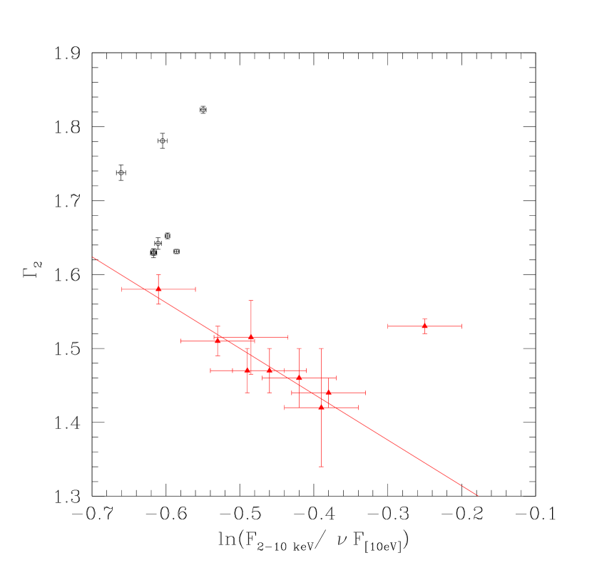
Figure 6: 2 – 10 keV spectral photon index of the phemenological model as a function of the logarithm of the ratio of the 2–10 keV to ultraviolet fluxes. Old Ginga and EXOSAT data are shown with red triangles. The line indicates the best correlation found in Walter & Courvoisier (1992). New XMM-Newton data are shown with black circles. We have extrapolated the UV spectrum obtained with the XMM optical monitor up to 10 eV using the time-averaged UV spectrum of 3C 273.

Figure 6 clearly shows that the correlations seen in EXOSAT/GINGA X-ray data and IUE UV data are not present in our data set. For completeness we have extended the analysis for the whole set of publicly available XMM-Newton data on 3C 273 to produce this Figure (for details see Soldi et al., in preparation).

In Fig. 6 two important facts are apparent. First, the scatter of the XMM-Newton data points along the x-axis is much smaller than that of the EXOSAT/GINGA and IUE points. This means that in the recent past the X-ray and UV fluxes have varied in a correlated way. Left top panel of Fig. 8 shows that this is indeed the case (Spearman correlation coefficient is equal to $R=0.93$, with a probability of random coincidence $P_{rand}=3\times 10^{-3}$). This is a quite surprising result, because previous searches for such correlations gave negative results. However another correlation typical for Seyfert galaxies between the hard X-ray spectral index $\Gamma_{2}$ and the X-ray flux (Zdziarski et al. (2003), and references therein), is not observed (see Fig. 7). A similar result was found by Page et al. (2004).

Second, the values of the hard X-ray spectral index in XMM-Newton observations are systematically higher than those of the EXOSAT/GINGA data. This indicates that the spectral state of the source has evolved over the 30 years of X-ray observations (in the next section we discuss this in details). This may be linked to the “disappearance” of the correlations seen in EXOSAT, GINGA and IUE data and “appearance” of X-ray – UV flux correlations not detected before.

Having found a previously undetected correlation between UV and X-ray flux, we have searched for the presence of additional correlations, such as between the 0.2-1 keV and 3-10 keV fluxes (top right panel of Fig. 8), 0.2-1 keV and 20-60 keV fluxes (bottom left panel of Fig. 8) and 20-60 keV and 60-100 keV fluxes (bottom right panel of Fig. 8). One can see a clear correlation between 20-60 keV and 60-100 keV fluxes, indicating that both bands are dominated by one and the same physical component (e.g. powerlaw emission from the jet). On the other side, no or only marginal correlation in the two other cases shows that several physical mechanisms contribute to the emission in these energy bands.

Figure 7: The dependence of the hard X-ray photon index (derived from fitting the data in 2-100 keV energy range with a single power law, see table 4) on the 2–10 keV X-ray flux.

Figure 8: Flux-flux plots for different energy bands. On the right bottom panel one day averaged INTEGRAL data are shown. To reduce the scatter the data were rebinned by building the average of three adjacent original data points in x direction.

4 Long-term evolution of the X-ray spectrum of 3C 273

To test the evolution of the X-ray spectrum over the last 30 year period we have collected the archival X-ray data from different missions. The evolution of the hard (2-10 keV) spectral index found from the archival data (Türler et al., 1999) is shown in Fig. 9. One clearly sees both significant short-term variations of the spectral index with a scatter of $\Delta\Gamma\simeq 0.1$ and a long-term trend of softening of the spectrum by as much as $\Delta\Gamma\simeq 0.4$ over the last 30 yr. It is interesting to note that during our 2003-2005 monitoring campaign the source has reached its historically softest hard X-ray spectrum characterized by a photon index $\Gamma=1.82\pm 0.01$. It is possible that still softer spectral states were found at the very beginning of X-ray observations (UHURU, ARIEL5/C and OSO8/A data points), but the uncertanity of those measurements are too large to be conclusive.

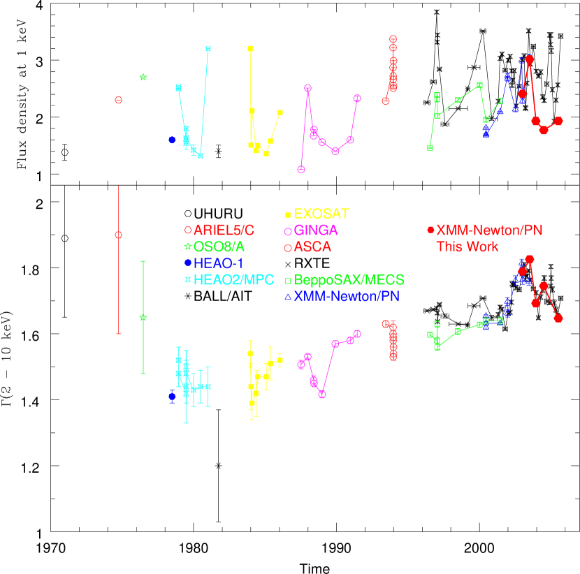
Figure 9: Evolution of the flux density at 1 keV, as extrapolated from the fit done above 2 keV, in $10^{-2}$photons/keV/cm${}^{2}/s$ (top panel) and hard X-ray spectral index (bottom panel) over the 30 years of observations. UHURU, Ariel 5/C, OSO 8/A, HEAO-1, HEAO-2/MPC, and BALL/AIT data points are taken from Malaguti et al. (1994); EXOSAT and Ginga data are taken from Turner et al. (1990); ASCA data are from Cappi et al. (1998); RXTE, Beppo-SAX, and part of XMM-Newton data are from Soldi et al. (in preparation).

5 Discussion

Most of the theoretical models of 3C 273 suggest that the source spectrum contains two major contributions, one from a pc-scale jet and the other from a Seyfert-like nucleus. The very low millimeter flux measured during our observations suggested that the jet contribution has reached its historical minimum (see Türler et al. (2006)). However, this did not result in the clear appearance of the Seyfert-like contribution. This means either that the Seyfert-like contribution has decreased simultaneously with the jet contribution (which, because of the difference in the size scales and production sites can happen only by a chance coincidence), or that the observed emission just can not be decomposed into Seyfert and jet contributions.

Our data show that the separation of Seyfert and jet contributions to the spectrum could not be done by fixing a ”template” for each of them. Namely, although the typical ranges of variations of soft and hard X-ray fluxes in our data set are similar to the ones of Beppo-SAX data set, the ”template” models for the Seyfert, jet and black body components found in our data set are significantly different. In particular, the additional black body component is not required by the data and thus the resulting black body flux shown in the left panel of Fig. 5 is systematically lower than the values reported in Grandi & Palumbo (2004). Our data show that the correlation between the black body and Seyfert components is absent at such low black body flux values. The same is true for the non-observation of the correlation between the Seyfert component flux and the strength of the iron line: since the addition of the iron line is not statistically required in any data sets except for the second one, no correlation is seen at such low iron line flux values. However, it is important to note that no direct comparison between our Fig. 5 and Fig. 1 of Grandi & Palumbo (2004) can be done, because of the differences in the template models derived from Beppo-SAX and INTEGRAL -XMM-Newton data sets.

In fact, the analysis of the secular evolution of the source presented above shows that both Seyfert and jet spectra evolve with time. This can be illustrated by the results presented in Fig. 6, where we plot the hard X-ray spectral slope as a function of the ratio of the X-ray power law flux to the UV flux. This ratio is apart from a constant factor the ratio of the Comptonized flux to the source photon flux in a model in which the X-ray power law is due to the Comptonization of the soft photons by a thermal electron population. The points given by the red crosses with large error bars were obtained by the EXOSAT and IUE missions in the 80-s and were analysed by Walter & Courvoisier (1992) who deduced that in the frame of the thermal Comptonization model, the electron temperature was about 1MeV or somewhat less. They also deduced that the optical depth of the Comptonizing medium was 0.1–0.2 and that it covered a couple of percent of the soft photon source.

The XMM-Newton data shown in Figure 6 by the black points with small error bars clearly do not match the correlation found in earlier years. This is particularly true for the spectra obtained during periods 1 and 2, when the soft X-ray emission was much brighter than at the other epochs, while the ultraviolet flux was similar. This indicates a much harder blue bump for these epochs. More photons were therefore available to Compton cool the hot electrons than inferred from the ultraviolet flux shown in Figure 5. This therefore leads to the softening in the X-ray emission. Alternatively, one can also infer a modification of the Comptonization region when the source is very weak. The recent data also show that the hard X-ray flux is correlated with the soft flux (see Figure 8), an effect not observed at earlier epochs (Courvoisier et al., 1990).

The correlation between the optical/UV and the X-ray flux is characteristic for Seyfert galaxies. This relationship is particularly clear in the long-term behaviour of NGC 5548 (Uttley et al., 2003), but was also seen in other Seyfert galaxies like for instance NGC 4051 (Shemmer et al. (2003), and references therein). The data of 3C 273 presented here do also show the appearance of such a trend (see Fig. 8), apparently suggesting a Seyfert-like behavior of 3C 273 in 2003–2005. However, it is clear from the above discussion that in the case of 3C 273 conclusions of this sort should be taken with caution: there is no clear way to disentangle the Seyfert and jet contributions. For example, another characteristic of Seyfert galaxies, a correlation between the hard X-ray spectral index $\Gamma_{2}$ and the X-ray flux (Zdziarski et al. (2003), and references therein), is not observed (see Fig. 7).

The secular evolution of the hard X-ray spectral index over the last 30 years, clearly seen in Fig. 9, shows that the jet contribution also evolves with time. Whether the hard X-ray flux is generated in the jet, or it is due to the nuclear related physics (i.e. from the ”compact source” (Lightman & Zdziarski, 1987)) is still completely undecided. ”Jet” and ”compact source” models differ in their approach to the so-called compactness problem. The essence of the compactness problem is that the naively estimated optical depth of the source for $\gamma$-rays with energies $E_{\gamma}$, such that pairs are produced in the interactions with soft photons of energies $\epsilon_{s}\geq 2m_{e}^{2}c^{4}/E_{\gamma}$, is higher than 1. The ”compact source” models self-consistently account for the effect of the pair production cascade in the source (Lightman & Zdziarski, 1987). The ”jet” models get rid of the compactness problem by assuming relativistic beaming of the $\gamma$-ray emission.

The observed evolution of the hard X-ray spectral index from $\Gamma\simeq 1.4$ to $\Gamma\simeq 1.8$ over the last 30 years could help to distinguish between the two possible models of the high-energy emission. The point is that although the present-day values $\Gamma>1.5$ are easily explained in both models, the very hard spectrum observed is the late 70-s is not. In both models the gamma-rays are produced via inverse Compton emission from high-energy electrons. The hard spectral index $\Gamma\simeq 1.4$ observed in 70-s and 80-s (see Fig. 9) is too hard for the optically thin inverse Compton emission from an electron distribution cooled via synchrotron and inverse Compton energy loss which can produce only spectra with $\Gamma\geq 1.5$.

This problem can, however, be relaxed if one assumes that in addition to electrons the emission region contains also protons. If the main source of the seed photons for the inverse Compton scattering is UV photons from the big blue bump, the hard X-ray inverse Compton emission originates from a population of electrons with moderate energies $E_{e}\sim 1-10$ MeV. In this energy range cooling could be dominated by ionization, rather than inverse Compton/synchrotron losses. The Coulomb loss leads to the hardening of the electron spectrum, compared to the injection spectrum by $\Delta\Gamma_{e}\simeq-1$. This will result in a hardening of the inverse Compton spectrum below the so-called ”Coulomb break” (see e.g. Aharonian (2004)). A simple estimate shows that if the proton density in the gamma-ray emission region is $n_{p}\sim 10^{10}\mbox{ cm}^{-3}$, the Coulomb break is situated in the hard X-ray band which can provide the explanation of the harder than $\Gamma=1.5$ spectrum of the source in late 70-s. High matter density in the emission region obviously favors the ”compact source” models compared to the jet models: the assumption about a large ($10^{10}$ cm^-3) matter densities at the pc distances from the nucleus needed to explain the hard spectrum in the jet model framework looks somewhat extreme (for comparison, the density of dust and molecular gas in the Central Molecular Zone (CMZ) of the Galaxy is estimated to be $10^{4}$ cm^-3, see e.g. Morris & Serabyn (1996)). The conclusion that the observed evolution of the hard X-ray spectral index favors the compact source models should also be taken with caution. The reason for this is that the presence of a Seyfert-like contribution to the hard X-ray spectrum can affect the value of the spectral index.

If the gamma-ray emission of 3C 273 originates in a compact source the synchrotron radiation from electrons which upscatter the blue bump photons to the GeV energy band could contribute also to the soft X-ray spectrum of the source. The magnetic field strength in the $\gamma$-ray emission region is poorly constrained by the observations (see, however, Courvoisier et al. (1988) for restrictions on the magnetic field strength during flaring activity of the source in the late 80-s). Assuming that the energy density of magnetic field in the compact emission region is comparable to the energy density of radiation,

$$U_{ph}\simeq 2\times 10^{2}\left[\frac{L}{10^{46}\mbox{erg/s}}\right]\left[\frac{10^{16}\mbox{cm}}{R}\right]^{2}\mbox{erg/cm}^{3}$$ (1)

(we estimate the size of emission region to be $R\sim 10^{16}$ cm from the observed intra-day variability of the source) one obtains an estimate

$$B\simeq 10^{2}\left[\frac{L}{10^{46}\mbox{erg/s}}\right]^{1/2}\left[\frac{10^{16}\mbox{cm}}{R}\right]\mbox{ G}$$ (2)

The synchrotron radiation from 1-10 GeV electrons in such magnetic field is emitted at the energies

$$\epsilon_{s}=3\left[\frac{B}{10^{2}\mbox{ G}}\right]\left[\frac{E_{e}}{10\mbox{ GeV}}\right]^{2}\mbox{ keV}$$ (3)

The non-observation of a cut-off in the GeV band (Collmar et al., 2000) implies that the high-energy cut-off in the electron spectrum is at least at energies $E_{e}\geq 1$ GeV which, in turn, implies that the cut-off in the synchrotron spectrum should be at least in the soft X-ray band. Taking into account that the best fit to the ”soft X-ray excess” in our data is given by a simple cut-off power law model, we find that it is possible that the observed soft X-ray excess in the spectrum of 3C 273 is the high-energy tail of the synchrotron radiation from the compact core of the source. As an example, we show in Fig. 10 a synchrotron-inverse Compton fit to the broad band spectrum of the source for the observation period 2 (with the historically steepest spectrum in the hard X-ray band). The parameters used for the model fit are: a magnetic field $B=33$ G, a size of emission region $R=10^{16}$ cm, a spectral index and cut-off in the electron spectrum are $\Gamma_{e}=2.6$ and $E_{cut}=10$ GeV, respectively. The gamma-ray spectrum has a break at $E=10$ MeV due to pair production. For comparison, short-dashed line in this figure shows the spectrum of inverse Compton emission without taking into account the pair production.

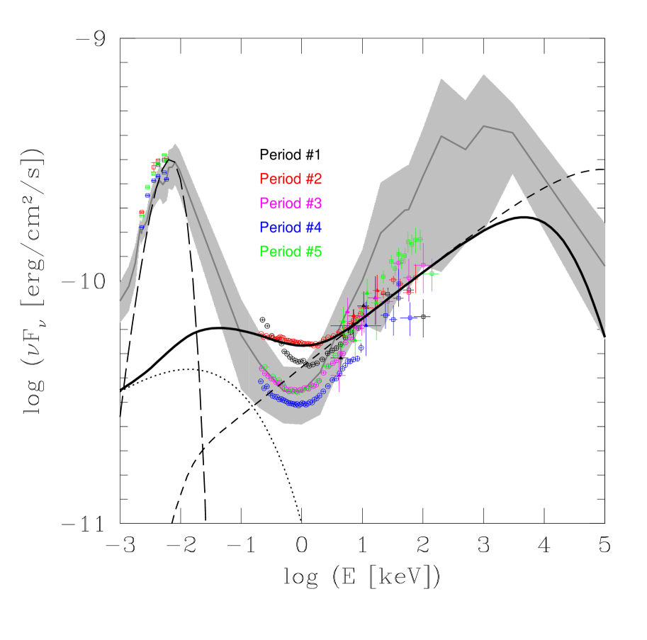
Figure 10: Synchrotron-external-Compton fits to the data for the observation period 2 in the ”compact source” type model. Solid line: the total spectrum, short dashed line: the inverse Compton spectrum without the account of the pair production. Dotted line: synchrotron spectrum. Long dashed line: the seed photon spectrum for the inverse Compton emission. Similar to Fig. 3 the average flux (grey line) and the 1-$\sigma$ variability range (grey area) is shown.

6 Summary

In this paper we have presented the results of monitoring of the quasar 3C 273 over the period of 2003–2005 over the broad energy band, spanning from optical/UV up to soft $\gamma$-rays with XMM-Newton and INTEGRAL. Our monitoring campaign gave some surprising results. In particular, in our data we find little support for the previously observed correlations between certain characteristics of the source, such as the ones found in Beppo-SAX data by Grandi & Palumbo (2004) (Fig. 5), and in GINGA/EXOSAT data by Walter & Courvoisier (1992)(Fig. 6). Moreover, we note the appearance of a new correlation between the UV and the X-ray flux from 3C 273, which was not present before. This points to the fact that the source undergoes a secular evolution. The secular evolution of the source is evident from the study of the evolution of the X-ray spectral index during the last 30 years of observations (Fig. 9). We argue that existing theoretical models have to be significantly modified to account for the observed spectral evolution of the source.

7 Acknowledgments

Authors are grateful to the unknown referee for helpful comments. PL acknowledges the support of KBN grant 1P03D01128.

References

- Aharonian (2004) Aharonian, F. A. 2004, Very high energy cosmic gamma radiation: a crucial window on the extreme Universe (published by World Scientific Publishing)
- Cappi et al. (1998) Cappi, M., Matsuoka, M., Otani, C., & Leighly, K. M. 1998, PASJ, 50, 213
- Collmar et al. (2000) Collmar, W., Reimer, O., Bennett, K., et al. 2000, A&A, 354, 513
- Courvoisier (1998) Courvoisier, T. J.-L. 1998, A&A Rev., 9, 1
- Courvoisier et al. (2003a) Courvoisier, T. J.-L., Beckmann, V., Bourban, G., et al. 2003a, A&A, 411, L343
- Courvoisier et al. (1990) Courvoisier, T. J. L., Robson, E. I., Blecha, A., et al. 1990, A&A, 234, 73
- Courvoisier et al. (1988) Courvoisier, T. J.-L., Robson, E. I., Hughes, D. H., et al. 1988, Nature, 335, 330
- Courvoisier et al. (2003b) Courvoisier, T. J.-L., Walter, R., Beckmann, V., et al. 2003b, A&A, 411, L53
- Crummy et al. (2006) Crummy, J., Fabian, A. C., Gallo, L., & Ross, R. R. 2006, MNRAS, 365, 1067
- Dickey & Lockman (1990) Dickey, J. M. & Lockman, F. J. 1990, ARA&A, 28, 215
- Grandi & Palumbo (2004) Grandi, P. & Palumbo, G. G. C. 2004, Science, 306, 998
- Lightman & Zdziarski (1987) Lightman, A. P. & Zdziarski, A. A. 1987, ApJ, 319, 643
- Malaguti et al. (1994) Malaguti, G., Bassani, L., & Caroli, E. 1994, ApJS, 94, 517
- Morris & Serabyn (1996) Morris, M. & Serabyn, E. 1996, ARA&A, 34, 645
- Page et al. (2004) Page, K. L., Turner, M. J. L., Done, C., et al. 2004, MNRAS, 349, 57
- Ross & Fabian (2005) Ross, R. R. & Fabian, A. C. 2005, MNRAS, 358, 211
- Shemmer et al. (2003) Shemmer, O., Uttley, P., Netzer, H., & McHardy, I. M. 2003, MNRAS, 343, 1341
- Türler et al. (2006) Türler, M., Chernyakova, M., Courvoisier, T. J.-L., et al. 2006, A&A, 451, L1
- Türler et al. (1999) Türler, M., Paltani, S., Courvoisier, T. J.-L., et al. 1999, A&AS, 134, 89
- Turner et al. (1990) Turner, M. J. L., Williams, O. R., Courvoisier, T. J. L., et al. 1990, MNRAS, 244, 310
- Uttley et al. (2003) Uttley, P., Edelson, R., McHardy, I. M., Peterson, B. M., & Markowitz, A. 2003, ApJ, 584, L53