VVDS-SWIRE

Abstract

Aims. By combining the VIMOS VLT Deep Survey (VVDS) with the Spitzer Wide-area InfraRed Extragalactic survey (SWIRE) data, we have built the currently largest spectroscopic sample of high redshift galaxies selected in the rest-frame near-infrared. In particular, we have obtained 2040 spectroscopic redshifts for a sample of galaxies with a magnitude measured at 3.6$\mu m$ $(m_{3.6})_{AB}<21.5$, and 1255 spectroscopic redshifts for a sample of galaxies with $(m_{4.5})_{AB}<21$. These allow us to investigate, for the first time using spectroscopic redshifts, the clustering evolution of galaxies selected from their rest-frame near-infrared luminosity, in the redshift range $0.2<z<2.1$.

Methods. We use the projected two-point correlation function $w_{p}(r_{p})$ to study the three dimensional clustering properties of galaxies detected at 3.6$\mu m$ and 4.5$\mu m$ with the InfraRed Array Camera (IRAC) in the SWIRE survey with measured spectroscopic redshifts from the first epoch VVDS. In addition, we measure the clustering properties of a larger sample of 16672 SWIRE galaxies for which we have accurate photometric redshifts on the same field by computing the angular correlation function. We compare these measurements.

Results. We find that in the flux limited samples at 3.6$\mu m$ and 4.5$\mu m$, the apparent correlation length does not change from redshift $\sim 2$ to the present. The measured correlation lengths have a mean value of $r_{0}\simeq 3.9\pm 0.5\leavevmode\nobreak\ h^{-1}\leavevmode\nobreak\ Mpc$ for the galaxies selected at 3.6$\mu m$ and a mean value of $r_{0}\simeq 4.4\pm 0.5\leavevmode\nobreak\ h^{-1}\leavevmode\nobreak\ Mpc$ for the galaxies selected at 4.5$\mu m$, all across the redshift range explored. These values are larger than those typicaly found for I-band selected galaxies at $I_{AB}<24$, for which $r_{0}$ varies from $2.69\leavevmode\nobreak\ h^{-1}\leavevmode\nobreak\ Mpc$ to $3.63\leavevmode\nobreak\ h^{-1}\leavevmode\nobreak\ Mpc$ between $z=0.5$ to $z=2.1$. We find that the difference in correlation length between I-band and $3.6-4.5\mu$m selected samples is decreasing with increasing redshift to become comparable at $z\simeq 1.5$. We interpret this as evidence that galaxies with older stellar populations and galaxies actively forming stars reside in comparably over-dense environments at epochs earlier than $z\simeq 1.5$, supporting the recently reported flattening of the color-density relation at high redshift. The increasing difference with cosmic time in correlation length observed between rest-frame UV-optical and near-infrared selected samples could then be an indication that star formation is gradually shifting to lower density regions as cosmic time increases, while the older passively evolving galaxies remain to trace the location of the highest primordial peaks.

1 Introduction

According to the current cosmological paradigm, the formation of large scale structures can be described as the evolution of primordial dark matter mass density perturbations under the influence of gravity. The galaxies that we observe are the result of the cooling and fragmentation of gas within the potential wells provided by the dark matter halos, that hierarchically build-up (White & Rees 1978). Even if the distribution of galaxies is in some way biased with respect to the distribution of the dark matter (Kaiser 1984), the spatial distribution of galaxies should therefore trace the dark matter density field. It is to be expected that the physical processes that build galaxies of different types and luminosities are sensitive to the mass of halos and their different environments. Therefore the evolution of the clustering of galaxies may depend on galaxy type, luminosity and environment. The comparison of the clustering of different galaxy populations along cosmic time could therefore provide useful constraints on the evolution and formation scenario of galaxies.
When galaxies are observed from redder wavelengths and up to a few microns rest-frame, this preferentially selects older stellar populations formed earlier in the life of the Universe. As the oldest stars are likely to have formed in the highest density peaks in the Universe, it is therefore expected that the clustering of their host galaxies would be significantly higher than that of galaxies hosting more recently formed stars. In the local Universe, selecting galaxies at 2.15 microns ($K_{s}$ band) from the Two Micron All Sky Survey (2MASS, Maller et al. 2005), it is found that these galaxies are more clustered than those selected at optical wavelengths, with an angular correlation amplitude several times larger than found in the Sloan Digital Sky Survey Early Data Release (SDSS EDR, Connolly et al. 2002), even if part of this difference may be due to the different luminosities of the samples. At higher redshifts, Oliver et al. (2004), based on Spitzer data, found that at $z_{median}\simeq 0.75$ the correlation length of $(m_{3.6})_{AB}<20.1$ (or equivalently $K_{Vega}<18.7$) selected galaxies is $r_{0}=4.4\pm 0.1\leavevmode\nobreak\ h^{-1}\leavevmode\nobreak\ Mpc$ with an angular correlation amplitude $\sim 60$ times lower than for 2MASS local galaxies, and the more luminous galaxies are even more strongly clustered (Farrah et al. 2006).
The IRAC 3.6$\mu m$ and 4.5$\mu m$  bands are only marginally affected by the first polycyclic aromatic hydrocarbon (PAH) spectral feature at 3.3$\mu m$, which fall in these bands in the redshift ranges [0,0.18] and [0.21,0.51] respectively. However, galaxy populations observed in these bands contain a mix of early-type, dust-reddened, and star-forming systems (Rowan-Robinson et al. 2005) which make clustering expectations less straightforward.
This paper aims to characterize the evolution of the real-space correlation length $r_{0}$ of near-infrared selected galaxies from the Spitzer Wide-area InfraRed Extragalactic survey (SWIRE, Lonsdale et al. 2003), which have secure spectroscopic redshifts from the VIMOS VLT Deep Survey (VVDS, Le Fèvre et al. 2005b). We compare these measurements to those in shallower samples, e.g. Oliver et al. (2004), as well as to the observed evolution of optically-selected galaxies as shown in Le Fèvre et al. (2005a), up to $z\simeq 2$.
In Section 2 we describe the galaxy sample that we use for this analysis. We present in Section 3 the formalism of the two-point correlation function and the results. Finally in Section 4 we discuss the observed clustering evolution and we conclude.
Throughout this analysis we assume a flat $\Lambda CDM$ cosmology with $\Omega_{M}=0.3$, $\Omega_{\Lambda}=0.7$, $\sigma_{8}=0.9$ and $H_{0}=100\leavevmode\nobreak\ h\leavevmode\nobreak\ km\cdot s^{-1}\cdot Mpc^{-1}$, while a value of $H_{0}=70\leavevmode\nobreak\ km\cdot s^{-1}\cdot Mpc^{-1}$ is used when computing absolute magnitudes.

2 The VVDS-SWIRE sample

The VVDS-SWIRE field is the intersection of the VIRMOS Deep Imaging Survey (VDIS, Le Fèvre et al. 2004) and the SWIRE-XMM/LSS fields, the total area covered on the sky is $\sim 0.82\leavevmode\nobreak\ deg^{2}$. From this field we extract two galaxy samples. The largest one consists of those SWIRE galaxies present in the field for which we measured photometric redshifts, called in the following the photometric redshift sample. The technique that we use to measure photometric redshifts is presented in the next section. The other sample, hereafter the spectroscopic redshift sample, contains galaxies included in a sub-area of $\sim 0.42\leavevmode\nobreak\ deg^{2}$ which corresponds to a fraction of the VVDS-Deep survey (Le Fèvre et al. 2005b) area and for which we have spectroscopic redshifts measured during the VVDS first epoch observations. We restrict this sample to galaxies with secure redshifts, i.e. with a redshift confidence level greater than $80\%$ (flag 2 to 9, Le Fèvre et al. 2005b). About 25% of the galaxy population is randomly sampled and we are correcting the correlation measurements for geometrical effects, e.g. on small scales, as described in Section 3 and in Pollo et al. (2005). In these two samples the star-galaxy separation has been performed first by using optical and mid-infrared colors to define the locus of galactic stars. In addition we used the spectral energy distribution (SED) template fitting procedure to reject any remaining stars and QSO. Objects which are best fitted with a star or a QSO SED template and which have a high SExtractor (Bertin & Arnouts 1996) stellarity index in the i’ band (CLASS_STAR $>0.97$) have been removed from the samples. The full description of the data-set and its properties is given in Le Fèvre et al. (2007, in preparation).

2.1 Photometric redshifts

The photometric redshifts have been estimated using the $\chi^{2}$ fitting algorithm Le Phare and calibrated with the VVDS first epoch spectroscopic redshifts on the same data-set as described in Ilbert et al. (2006), including in addition the 3.6$\mu m$ and 4.5$\mu m$ infrared photometry from SWIRE (Lonsdale et al. 2003). The photometric data cover the wavelength domain $0.3\mu m\leq\lambda\leq 5.0\mu m$ including B,V,R,I from VDIS (Le Fèvre et al. 2004), u*,g’,r’,i’,z’ from the Canada France Hawaii Telescope Legacy Survey (CFHTLS-D1, McCracken et al., in preparation), K-band from VDIS (Iovino et al. 2005) and the 3.6$\mu m$ and 4.5$\mu m$ infrared photometry from SWIRE (Lonsdale et al. 2003). The empirical templates used by Ilbert et al. (2006) have been extended to the mid-infrared domain using the GISSEL library (Bruzual & Charlot 2003) and we use the spectroscopic sample to simultaneously adapt the templates and the zero-point calibrations (Ilbert et al. 2006). The comparison with 1500 spectroscopic redshifts from the VVDS first epoch data shows an accuracy of $\sigma_{\Delta z/(1+z)}\simeq 0.031$ with a small fraction of catastrophic errors: $1.7\%$ objects with $|\Delta z|>0.15(1+z)$, up to a redshift $z\sim 2$. The full description of the method and the data used to compute these photometric redshifts is given in Ilbert et al. (2006) and Arnouts et al. (2007, in preparation).

2.2 Selection functions

We split the spectroscopic redshift and photometric redshift samples into two sub-samples, applying a simple magnitude selection from observed fluxes on the two first infrared photometric bands of the SWIRE survey, the Spitzer-IRAC 3.6$\mu m$ and 4.5$\mu m$ bands. These sub-samples satisfy respectively to a magnitude in the AB system measured in the 3.6$\mu m$ band of $(m_{3.6})_{AB}<21.5$ and in the 4.5$\mu m$ band of $(m_{4.5})_{AB}<21$ or, equivalently in flux, $S_{3.6}>9.2\leavevmode\nobreak\ \mu Jy$ and $S_{4.5}>14.5\leavevmode\nobreak\ \mu Jy$. These criteria correspond to the limits of completeness for the SWIRE bands (Le Fèvre et al., 2007, in preparation). In addition, the spectroscopic redshift sample has a $I_{AB}$ cut due to the fact that the VVDS-Deep spectroscopic sample is a magnitude-selected sample according to the criterion $17.5<I_{AB}<24$. The $I_{AB}$ cut introduces a color dependent incompleteness in terms of SWIRE magnitudes in the spectroscopic redshift sample. Indeed we loose a small fraction of objects which correspond to faint and red objects as shown in Figure 1 and Figure 2 for the 3.6$\mu m$ and 4.5$\mu m$ galaxies. We estimate the fraction of lost galaxies to be respectively $11.6\%$ and $10.3\%$. To understand the population missed in the spectroscopic sample, we have used the photometric redshifts described in the previous section. We find that the galaxies that we are missing in the 4.5$\mu m$ spectroscopic redshift sub-sample are redder than those in the 3.6$\mu m$ spectroscopic sub-sample. The median $(I-m_{3.6})_{AB}$ color of these sub-samples are $3.72$ and $3.67$ respectively, as shown in Figure 3. We note that photometric redshifts may have difficulties in identifying dust obscured AGN because we are lacking the redder bands like the Spitzer-IRAC 24$\mu m$. However, the fraction of dust reddened AGN is expected to be low (Tajer et al. 2007), and its impact on clustering properties must be insignificant. Therefore, the photometric redshift sample, which is assumed to be complete and free of significant contaminants, allows us to evaluate the effect of the color dependent magnitude incompleteness on the clustering measurements performed on the spectroscopic redshift sample.

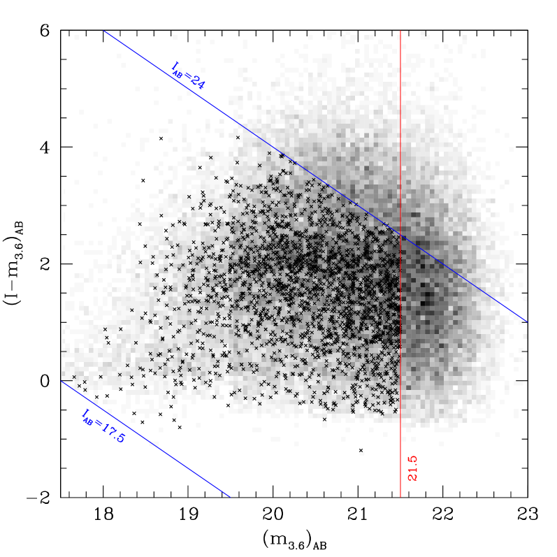
Figure 1: Color-magnitude diagram for the 3.6$\mu m$ spectroscopic and photometric sub-samples. All the galaxies detected at 3.6$\mu m$ in the VVDS-SWIRE field are represented in grey scale. The photometric redshift sub-sample consists of all the objects with $(m_{3.6})_{AB}<21.5$ and galaxies from the spectroscopic sub-sample are shown as crosses. The vertical line indicates the limit of completeness and the two diagonal lines show the limits of the spectroscopic selection $17.5<I_{AB}<24$. We estimate that the fraction of galaxies we lose in the spectroscopic redshift sub-sample due to the VVDS spectroscopic selection and assuming the completeness limit $(m_{3.6})_{AB}<21.5$, is 11.6%.

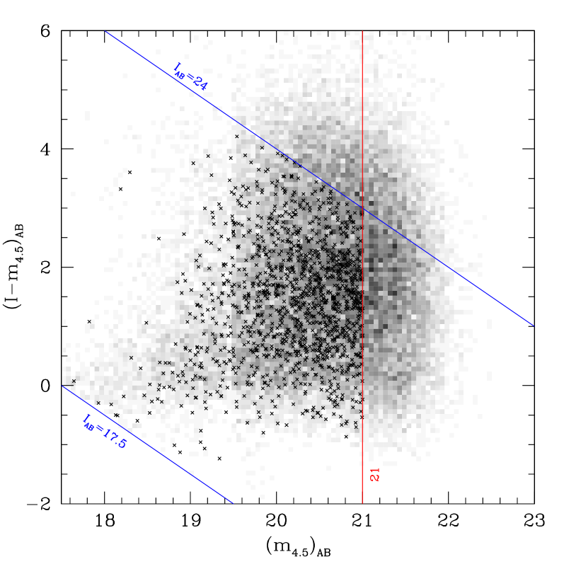
Figure 2: Color-magnitude diagram for the 4.5$\mu m$ spectroscopic and photometric sub-samples. All the galaxies detected at 4.5$\mu m$ in the VVDS-SWIRE field are represented in grey scale. The photometric redshift sub-sample consists of all the objects with $(m_{4.5})_{AB}<21$ and galaxies from the spectroscopic sub-sample are shown as crosses. The vertical line indicates the limit of completeness and the two diagonal lines show the limits of the spectroscopic selection $17.5<I_{AB}<24$. We estimate that the fraction of galaxies we lose in the spectroscopic redshift sub-sample due to the VVDS spectroscopic selection and assuming the completeness limit $(m_{4.5})_{AB}<21$, is 10.3%.

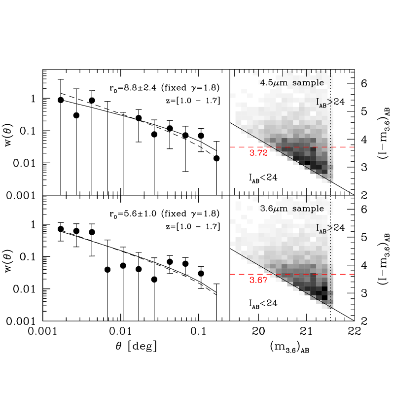
Figure 3: The right panels present the color-magnitude diagrams $(I-m_{3.6})_{AB}$ versus $(m_{3.6})_{AB}$ for the 3.6$\mu m$ (top) and 4.5$\mu m$ (bottom) photometric sub-samples considering the objects that fall above the spectroscopic selection upper limit $I_{AB}=24$. The galaxy number density is shown in grey scale and the dashed line indicates the median of the $(I-m_{3.6})_{AB}$ distributions. In the left panels are shown the angular correlation function for these two selections in the redshift range $z_{phot}=[1,1.7]$. In these panels the solid lines show the best-fit model when letting the two parameters free, while the dashed lines indicate the best-fit model with fixed $\gamma=1.8$.

3 Clustering measurements

3.1 Methods

3.1.1 Computing the projected correlation function

The method applied to compute the projected correlation function and to derive the real-space correlation length $r_{0}$ and the correlation function slope $\gamma$, is described extensively in Pollo et al. (2005). We present in this section the main points of the method.
First we evaluate the bi-dimensional two-point correlation function $\xi(r_{p},\pi)$ using the standard Landy and Szalay estimator (Landy & Szalay 1993). This estimator of the two-point correlation function is defined by:

$$\xi(r)=\frac{GG(r)-2GR(r)+RR(r)}{RR(r)}$$ (1)

where $GG(r)$, $RR(r)$ and $GR(r)$ are the normalized numbers of independent galaxy-galaxy, galaxy-random and random-random pairs with comoving separation between $r$ and $r+dr$. The three-dimensional galaxy space distribution recovered from a redshift survey and its two-point correlation function $\xi(s)$, are distorted due to the effect of galaxy peculiar velocities. Therefore the redshift-space separation $s$ differs from the true physical comoving separation $r$. These distortions occur only radially since peculiar velocities affect only redshift. Thus we compute the bi-dimensional two-point correlation $\xi(r_{p},\pi)$ by splitting the separation vector $s$ into two components: $r_{p}$ and $\pi$, respectively perpendicular and parallel to the line of sight (Fisher et al. 1994). In this way, we separate the redshift distortions from the true spatial correlations.
Then, we project $\xi(r_{p},\pi)$ along the line of sight, onto the $r_{p}$ axis. This allows to integrate out the dilution produced by the redshift-space distortion field and we obtain the projected two-point correlation function, which is defined by,

$$w_{p}(r_{p})=2\int_{0}^{\infty}\xi(r_{p},\pi)d\pi=2\int_{0}^{\infty}\xi\left(\sqrt{r_{p}^{2}+y^{2}}\right)dy$$ (2)

In practice, the upper integration limit has to be finite to avoid noise, therefore we choose its optimal value as $20\leavevmode\nobreak\ h^{-1}\leavevmode\nobreak\ Mpc$ (Pollo et al. 2005). Assuming a power-law form for $\xi(r)$, i.e. $\xi(r)=\left(r_{0}/r\right)^{\gamma}$, one can write $w_{p}(r_{p})$ as,

$$w_{p}(r_{p})=r_{p}\left(\frac{r_{0}}{r_{p}}\right)^{\gamma}\frac{\Gamma\left(\frac{1}{2}\right)\Gamma\left(\frac{\gamma-1}{2}\right)}{\Gamma\left(\frac{\gamma}{2}\right)}$$ (3)

where $\Gamma$ is the Euler Gamma function.
We fit the $w_{p}(r_{p})$ measurements to a power-law model (equation 3) by minimizing the generalized $\chi^{2}$. The advantage of this method is that it takes into account the fact that the different points of the correlation function are correlated. We define the generalized $\chi^{2}$ in our case as (Pollo et al. 2005),

$$\chi^{2}=\sum_{i=1}^{N_{p}}\sum_{j=1}^{N_{p}}(w^{mod}_{p}(r_{i})-w^{obs}_{p}(r_{i}))C^{-1}_{ij}(w^{mod}_{p}(r_{j})-w^{obs}_{p}(r_{j}))$$ (4)

where $w_{p}^{mod}(r_{i})$ ($w_{p}^{obs}(r_{i})$) is the value of $w_{p}^{mod}$ ($w_{p}^{obs}$) computed at $r_{p}=r_{i}$ with $1<i<N_{p}$ ($N_{p}$ is the number of $r_{p}$ points), and $C$ is the covariance matrix of the data estimated using bootstrap re-sampling. 100 bootstrap samples have been used in this analysis. The error bars estimated from the covariance matrix associated to the bootstrap samples include the statistical error only and do not take into account the error due to cosmic variance. Therefore, in order to have a realistic estimation of the errors bars on our measurements, we compute $w_{p}(r_{p})$ on 50 mock VVDS surveys constructed using the GalICS simulation (Hatton et al. 2003). This simulation of hierarchical galaxy formation is based on a hybrid N-body/semi-analytic model and is particularly well adapted to simulate the properties of the high-redshift galaxies that we observe in the VVDS (Blaizot et al. 2005; Pollo et al. 2005). Moreover, the selection function and the observational biases present in the VVDS dataset have been included in these mock samples (Pollo et al. 2005). Thus we fit the $w_{p}(rp)$ measurements from the simulations using the same method as described previously and we estimate the confidence limits on the $r_{0}$ and $\gamma$ measurements looking at the $\Delta\chi^{2}$ distribution from the best fit (Pollo et al. 2005). The error bars obtained using this method are larger but more realistic than those from the bootstrap method. They include not only the statistical error but also the error which comes from the cosmic variance, which dominates here.

3.1.2 Computing the angular correlation function

In order to compute the angular two-point correlation function $w(\theta)$ (ACF), we use the Landy & Szalay estimator presented in equation 1, but in this case, simply considering angular pairs. Assuming that $w(\theta)$ is well described by a power-law model as $w(\theta)=A_{w}\theta^{1-\gamma}$, we fit the measured ACF to this model using the generalized $\chi^{2}$ method and deduce the amplitude $A_{w}$ and the slope $1-\gamma$. Because of the finite size of the survey, we introduce the integral constraint (IC) correction in our fitting procedure. It is defined as follows (Roche et al. 1993),

$$IC=\int\!\!\!\int{\frac{w(\theta)}{\Omega^{2}}d\Omega_{1}d\Omega_{2}}=\frac{A_{w}}{\Omega^{2}}\int\!\!\!\int{\theta^{1-\gamma}d\Omega_{1}d\Omega_{2}}=A_{w}B(\gamma)$$ (5)

with,

$$B(\gamma)=\frac{1}{\Omega^{2}}\int\!\!\!\int{\theta^{1-\gamma}d\Omega_{1}d\Omega_{2}}$$ (6)

where $\Omega$ is the area of the observed field. We compute $B(\gamma)$ by numerically integrating this expression over the entire data area excluding regions where there are photometric defects. At the end our measurements are fitted with the expression:

$$w_{mod}(\theta)=A_{w}\theta^{1-\gamma}-IC=A_{w}(\theta^{1-\gamma}-B(\gamma))$$ (7)

In order to derive the real-space correlation length $r_{0}$ from the angular correlation amplitude $A_{w}$, we use the Limber deprojection technique as described in Magliocchetti & Maddox (1999). This method, which is based on the Limber relativistic equation (Limber 1953), permits to recover the value of $r_{0}$ given $A_{w}$ and the redshift distribution of the galaxies. In general, this technique is not very stable and the shape of the redshift distribution that one considers is critical, but in this study, we measure ACF in relatively narrow redshift bins so the shape we assume for the inversion is not so critical. We use a smoothed redshift distribution by applying a moving window with a width of $\Delta z=0.2$ to the initial photometric redshift distribution (Le Fèvre et al., 2007, in preparation). The width of the smoothing window has been chosen to reflect the typical uncertainty that we have on the photometric redshift values. The ACF error bars have been estimated using the bootstrap re-sampling method.

3.2 Clustering results

3.2.1 Clustering of the spectroscopic redshift sample

We compute $w_{p}(r_{p})$ in increasing spectroscopic redshift slices from $z=0.2$ to $z=2.1$. Therefore we divide the 3.6$\mu m$ sub-sample in six redshift slices: $[0.2,0.5]$, $[0.5,0.7]$, $[0.7,0.9]$, $[0.9,1.1]$, $[1.1,1.3]$, $[1.3,2.1]$. The 4.5$\mu m$ sub-sample has fewer objects than the 3.6$\mu m$ one because of the slightly shallower depth. In order to maximize the number of objects per redshift slice, we consider in this case three slices only: $[0.2,0.7]$, $[0.7,1.1]$ and $[1.1,2.1]$.
In the fitting procedure, we use all the $w_{p}(r_{p})$ points for $0.1\leq r_{p}\leq 12\leavevmode\nobreak\ h^{-1}\leavevmode\nobreak\ Mpc$. The projected correlation functions computed in each redshift slice are plotted in Figure 4 with the contours of confidence for the best-fitted parameters. Table 1 summarizes the values of the correlation length and the correlation function slope that we derive for the two sub-samples of the spectroscopic redshift sample.

Table 1: VVDS-SWIRE spectroscopic redshift sample: sub-sample properties and associated measurements of the slope, the correlation length and the linear bias.

Spectroscopic redshift sample
Sub-sample	Redshift	Mean	Number	$\langle M_{B}\rangle_{Vega}$	$\gamma$	$r_{0}$ ($h^{-1}\leavevmode\nobreak\ Mpc$)	$r_{0}$ ($h^{-1}\leavevmode\nobreak\ Mpc$)	$b_{L}$
	interval	redshift	of galaxies				(fixed $\gamma=1.8$)
3.6$\mu m$	$[0.2,0.5]$	0.36	336	-19.53	$1.92^{+0.27}_{-0.18}$	$3.8^{+0.6}_{-0.7}$	$3.9^{+0.6}_{-0.7}$	$0.93^{+0.10}_{-0.11}$
	$[0.5,0.7]$	0.60	445	-20.29	$1.88^{+0.21}_{-0.14}$	$4.2^{+0.5}_{-0.5}$	$4.4^{+0.5}_{-0.5}$	$1.15^{+0.10}_{-0.10}$
	$[0.7,0.9]$	0.81	512	-20.75	$1.77^{+0.15}_{-0.11}$	$3.8^{+0.4}_{-0.4}$	$3.7^{+0.4}_{-0.4}$	$1.15^{+0.09}_{-0.09}$
	$[0.9,1.1]$	0.99	385	-21.17	$1.87^{+0.17}_{-0.14}$	$4.2^{+0.4}_{-0.4}$	$4.3^{+0.4}_{-0.4}$	$1.38^{+0.11}_{-0.11}$
	$[1.1,1.3]$	1.19	195	-21.66	$2.44^{+0.22}_{-0.16}$	$3.8^{+0.5}_{-0.5}$	$3.7^{+0.5}_{-0.5}$	$1.62^{+0.43}_{-0.43}$
	$[1.3,2.1]$	1.57	93	-22.13	$2.19^{+0.37}_{-0.38}$	$5.8^{+0.7}_{-1.0}$	$7.6^{+0.7}_{-1.0}$	$2.55^{+0.76}_{-0.96}$
4.5$\mu m$	$[0.2,0.7]$	0.48	485	-20.22	$1.84^{+0.18}_{-0.16}$	$3.9^{+0.5}_{-0.5}$	$3.9^{+0.5}_{-0.5}$	$1.01^{+0.08}_{-0.08}$
	$[0.7,1.1]$	0.90	537	-21.15	$1.84^{+0.14}_{-0.14}$	$4.0^{+0.3}_{-0.4}$	$4.0^{+0.3}_{-0.4}$	$1.26^{+0.09}_{-0.10}$
	$[1.1,2.1]$	1.42	182	-21.97	$1.82^{+0.26}_{-0.22}$	$3.7^{+0.6}_{-0.7}$	$3.7^{+0.6}_{-0.7}$	$1.48^{+0.24}_{-0.28}$

Figure 4: ILeft panels: projected correlation functions for the 3.6$\mu m$ spectroscopic redshift sub-sample in different redshift slices with their best-fit power law. Right panels: the $68.3\%$, $90\%$ and $95.4\%$ confidence contours for the clustering parameters $r_{0}$ and $\gamma$.

The correlation length measured in the $3.6$$\mu m$ and $4.5$$\mu m$ sub-samples is roughly constant over the redshift range z=[0.2,2.1]. It varies slightly between $3.8$ and $4.2\leavevmode\nobreak\ h^{-1}\leavevmode\nobreak\ Mpc$, except in the high-redshift interval $[1.3,2.1]$ of the $3.6$$\mu m$ sub-sample where a large correlation length of $5.8\leavevmode\nobreak\ h^{-1}\leavevmode\nobreak\ Mpc$ is found. In this redshift range we are probing the intrinsically brightest galaxies, with a median absolute magnitude of $\langle M_{B}\rangle_{Vega}=-22.13$ (Table 1). Compared to the characteristic absolute magnitude $M^{*}_{B}$ at this redshift reported by Ilbert et al. (2005), it is found that for these objects, $\Delta M^{*}_{B}=\langle M_{B}\rangle-M_{B}^{*}\simeq-0.27$ and equivalently $\langle L_{B}\rangle/L^{*}_{B}\simeq 1.3$. Thus, these luminous galaxies are expected to be more strongly clustered as the halo clustering strength increases more rapidly for luminosities greater than a few times $L^{*}$ (Zehavi et al. 2005; Norberg et al. 2002). Indeed Pollo et al. (2006); Coil et al. (2006) have shown that the galaxy correlation length increases more steeply for magnitude brighter than $M^{*}$ at $z\simeq 1$ with $r_{0}$ values about $5\leavevmode\nobreak\ h^{-1}\leavevmode\nobreak\ Mpc$. Our high $r_{0}$ measurement in this high redshift bin is thus fully consistent with these findings. Moreover, in this redshift interval the 1.6$\mu m$ rest-frame emission feature from the photospheric emission of evolved stars (Simpson & Eisenhardt 1999), is present in the 3.6$\mu m$ band, favoring the detection of more massive and significantly more clustered systems (Farrah et al. 2006). We discuss in details the evolution of the correlation length for the two sub-samples in Section 4.

3.2.2 Clustering of the photometric redshift sample

We measure the ACF and deduce the clustering parameters $r_{0}$ and $\gamma$ on the photometric redshift sample in order to test the measurements from the spectroscopic redshift sample and to evaluate the effect of incompleteness.
With the same methodology we compute the ACF in increasing photometric redshift slices, selecting the slice boundaries in order to take the photometric redshift errors into account. We consider five slices with increasing size: $[0.2,0.5]$, $[0.5,0.7]$, $[0.7,1.0]$, $[1.0,1.3]$ and $[1.3,1.7]$. No redshift slices have been considered beyond $z_{phot}=1.7$ because the lack of accuracy of the photometric redshifts in this case seriously corrupts the measurements.
We fit the measured ACF to a power-law model over $0.0017\leq\theta\leq 0.1$ degrees, where the shape of the ACF is very close to a power law. However, it is evident in Figure 5 that the ACF departs from this model at scales greater than $\sim 0.1$ degrees in redshift slices with $z_{phot}>0.7$. The excess of power at large angular scale could be explained by the presence of another component in the correlation function or of the presence of residual inhomogeneities in the field. We will explore this point more in detail in a future paper as it does not impact the results presented here. The ACF for the different redshift slices are plotted in Figure 5. The best-fitted values of the angular correlation amplitude $A_{w}$, the correlation function slope $\gamma$ and the correlation length $r_{0}$ that we derive with the Limber deprojection technique, are reported in Table 2.

Table 2: VVDS-SWIRE photometric redshift sample: sub-sample properties and associated measurements of the ACF amplitude, the slope and the correlation length.

Photometric redshift sample
Sub-sample	Photometric	Mean redshift	Number of galaxies	$A_{w}\times 10^{3}$	$\gamma$	$r_{0}$ ($h^{-1}\leavevmode\nobreak\ Mpc$)	$r_{0}$ ($h^{-1}\leavevmode\nobreak\ Mpc$)
	redshift interval						(fixed $\gamma=1.8$)
3.6$\mu m$	$[0.2,0.5]$	0.37	2726	$7.7^{+4.7}_{-3.1}$	$1.76^{+0.10}_{-0.09}$	$4.2^{+1.5}_{-1.0}$	$4.0^{+0.3}_{-0.3}$
	$[0.5,0.7]$	0.60	2714	$7.1^{+4.5}_{-3.0}$	$1.83^{+0.10}_{-0.09}$	$4.1^{+1.4}_{-0.9}$	$4.2^{+0.3}_{-0.3}$
	$[0.7,1.0]$	0.85	5110	$1.2^{+0.8}_{-0.5}$	$2.03^{+0.11}_{-0.11}$	$2.8^{+1.0}_{-0.6}$	$3.4^{+0.2}_{-0.2}$
	$[1.0,1.3]$	1.14	3577	$5.1^{+4.0}_{-2.5}$	$1.81^{+0.12}_{-0.11}$	$4.3^{+1.9}_{-1.1}$	$4.3^{+0.3}_{-0.3}$
	$[1.3,1.7]$	1.47	2545	$3.4^{+3.7}_{-1.9}$	$1.83^{+0.16}_{-0.15}$	$4.0^{+2.4}_{-1.2}$	$4.1^{+0.4}_{-0.4}$
4.5$\mu m$	$[0.2,0.5]$	0.37	1977	$7.6^{+4.3}_{-2.8}$	$1.79^{+0.09}_{-0.10}$	$4.4^{+1.4}_{-0.9}$	$4.3^{+0.3}_{-0.3}$
	$[0.5,0.7]$	0.60	1708	$10.4^{+8.5}_{-4.9}$	$1.80^{+0.13}_{-0.12}$	$4.8^{+2.2}_{-1.2}$	$4.8^{+0.3}_{-0.3}$
	$[0.7,1.0]$	0.85	2971	$1.1^{+1.0}_{-0.5}$	$2.10^{+0.12}_{-0.13}$	$3.0^{+1.4}_{-0.7}$	$4.0^{+0.3}_{-0.3}$
	$[1.0,1.3]$	1.14	2287	$6.1^{+7.1}_{-3.3}$	$1.81^{+0.15}_{-0.16}$	$4.8^{+3.1}_{-1.4}$	$4.8^{+0.4}_{-0.4}$
	$[1.3,1.7]$	1.47	1700	$4.3^{+5.9}_{-2.5}$	$1.79^{+0.17}_{-0.19}$	$4.3^{+3.2}_{-1.4}$	$4.2^{+0.5}_{-0.5}$

Figure 5: The angular correlation function as a function of redshift, for the 3.6$\mu m$ and 4.5$\mu m$ photometric redshift sub-samples. The solid lines show the best-fit model when letting the two parameters free, while the dashed lines indicate the best-fit model with fixed $\gamma=1.8$.

Given the uncertainties on the ACF measurements, we adopt a fixed slope $\gamma=1.8$. This is supported by the fact that when letting both $r_{0}$ and $\gamma$ vary in the ACF fitting, we find $\gamma$ values very similar to 1.8, while the errors on $r_{0}$ increase slightly.
The values of the correlation length that we derive for the 3.6$\mu m$ and 4.5$\mu m$ photometric samples do not evolve with redshift up to $z_{phot}=1.7$. In the case of the 3.6$\mu m$ sub-sample, the $r_{0}$ values are in good agreement with the values found in the spectroscopic redshift sample given the size of the error bars. We observe slightly larger values of the correlation length for the 4.5$\mu m$ photometric redshift sub-sample than for the 4.5$\mu m$ spectroscopic redshift one. We interpret this as an effect of the incompleteness of the spectroscopic samples due to the I-band selection. To test this we have measured on the photometric sample the clustering of the red population which is missed by the spectroscopic sample in each of the 3.6$\mu m$ and 4.5$\mu m$ bands. As most of the missed population in both cases is at redshifts $z_{phot}>1$, we have been able to perform this analysis only in the redshift range $z_{phot}=[1,1.7]$ where the available number of galaxies is large enough for a clustering signal to be measured. Results are presented in Figure 3. We find that the clustering of the missed red population in the 3.6 microns spectroscopic sample has a correlation length of $r_{0}=5.6\pm 1.0$ only marginally larger than that of the bulk of the population, and therefore the clustering signal of the photometric and spectroscopic samples are found to be very similar. For the red population in the 4.5 microns sample, we find that $r_{0}=8.8\pm 2.4$, a significantly larger value that the main population. This explains why the spectroscopic sample slightly underestimates the clustering signal when compared to the photometric sample.

4 Discussion and conclusions

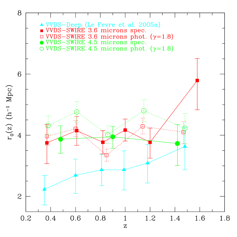
Figure 6: Clustering evolution of VVDS-SWIRE samples of near-infrared galaxies compared to the VVDS-Deep I-band measurements. Filled symbols refer to measurements from spectroscopic samples while open symbols refer to measurements from photometric samples.

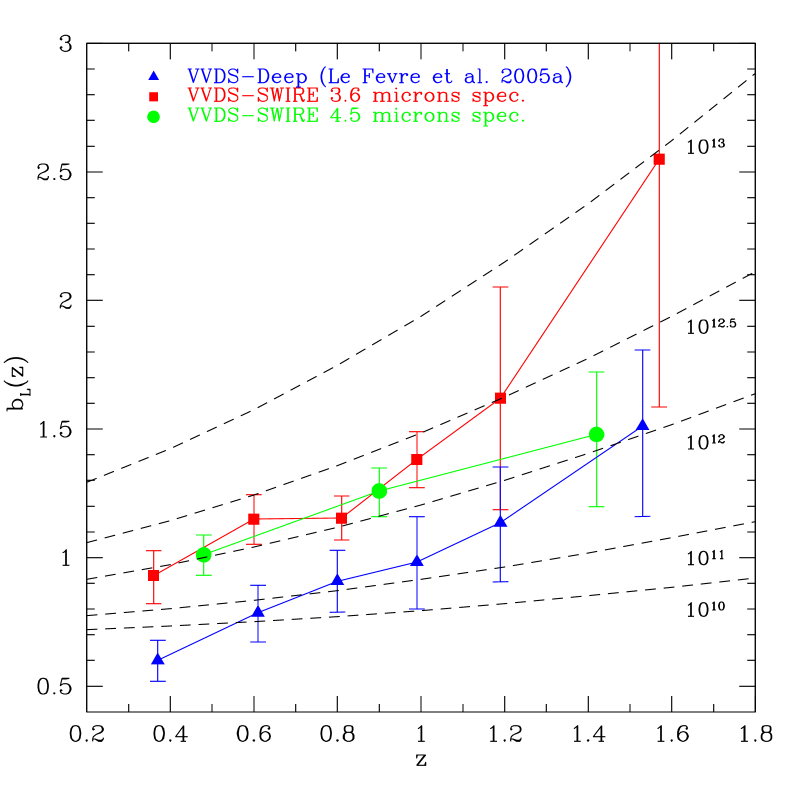
Figure 7: Trend of the linear bias as a function of redshift for the VVDS-SWIRE 3.6$\mu m$ and 4.5$\mu m$ spectroscopic redshift samples compared to the VVDS-Deep I-band one. The dashed curves show the theoritical linear halo bias evolution for dark matter halos of mass greater than $10^{10},10^{11},10^{12},10^{12.5}$ and $10^{13}h^{-1}M_{\odot}$ (from bottom to top). The linear galaxy bias is computed as described in Magliocchetti et al. (2000) from the $r_{0}$ and $\gamma$ measurements. The theoretical curves have been computed using the fitting functions of Sheth & Tormen (1999) for the halo mass function and bias.

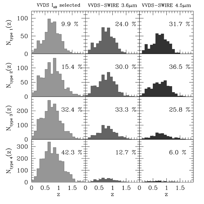
Figure 8: Redshift distribution per spectral types for the 3.6$\mu m$ and 4.5$\mu m$ spectroscopic redshift sub-samples compared to the VVDS-Deep sample. We use the spectral types defined in Zucca et al. (2006): type 1 corresponds to E/S0, type 2 to early spiral, type 3 to late spiral and type 4 to irregular/starburst galaxies.

We first compare our measurements with previously reported results on samples of galaxies selected using Spitzer-IRAC bands. Oliver et al. (2004) use a similar type of galaxy selection, as they define a flux-limited sample of SWIRE galaxies with $S_{3.6}>32\mu Jy$, and they compute the ACF and deduce $r_{0}$ using Limber deprojection assuming a parametrized redshift distribution. The selection criterion they consider is different from the one we use, i.e. $S_{3.6}>9.2\mu Jy$. This selects brighter galaxies than in our sample, that are expected to be more strongly clustered (Pollo et al. 2006; Coil et al. 2006). They find a correlation length $r_{0}=4.4\pm 0.1\leavevmode\nobreak\ h^{-1}\leavevmode\nobreak\ Mpc$ at $z\simeq 0.75$ with $\gamma=1.8$, which is higher than our value of $r_{0}=3.7\pm 0.4\leavevmode\nobreak\ h^{-1}\leavevmode\nobreak\ Mpc$ at $z\simeq 0.81$. Taking into account that galaxies in their sample are 1.4 magnitudes brighter and that brighter galaxies are on average more clustered, the two results are found to be in good agreement.
We then compare our results with the clustering measurements of I-band selected VVDS-Deep galaxies (Le Fèvre et al. 2005a) in the same area. This comparison is shown in Figure 6, where the correlation length for the different samples is plotted. We observe that the correlation length is globally higher for near-infrared selected galaxies compared to optically-selected ones and that it is roughly constant over the redshift range $z=[0.2,2.1]$. By comparison, $r_{0}$ from the I-selected sample shows a steady increase with redshift. As discussed in Section 3, the clustering of the 4.5$\mu m$-selected galaxy population is higher as measured from the photometric sample than from the spectroscopic sample because the latter misses a significant fraction of red galaxies due to the additional $17.5<I_{AB}<24$ cut applied by the VVDS-Deep survey selection. When comparing the measurements at 3.6$\mu m$  and 4.5$\mu m$  obtained from the photometric sample (open symbols in Figure 6), we observe that the clustering of the sample selected at the reddest wavelength is slightly stronger, although comparable given the errors. This is expected, as selecting from longer wavelengths we are sampling preferentially more early-types than later ones as described below. The color dependency of the clustering of galaxies in the VVDS-SWIRE sample will be reported elsewhere (de la Torre et al., in preparation).
In order to understand the systematically higher values of clustering that we find compared to those from optically-selected galaxies and to quantify the type of galaxy population included in our near-infrared samples, we derive the spectral types of our spectroscopic redshift sample galaxies using the galaxy classification introduced by Zucca et al. (2006). This classification is based on the match to an empirical set of spectral energy distributions (as described in Arnouts et al. 1999) of the galaxy rest-frame colors, obtained from the multi-wavelength information and spectroscopic redshift. The redshift distributions per galaxy types are presented in Figure 8 for the I-band, 3.6$\mu m$ and 4.5$\mu m$ selected samples. The four spectral types defined as type 1 to 4 correspond respectively to E/S0, early spiral, late spiral and irregular/starburst galaxies. One can see in Figure 8 that the VVDS-Deep I-selected sample is dominated by late types (type 3 and 4) whereas the 4.5$\mu m$ selected sample is dominated by early types (type 1 and 2). In the 3.6$\mu m$ sample the different types balance out. Early type galaxies are known to be more clustered than late type ones at $z=0$ (e.g. Norberg et al. 2002; Zehavi et al. 2005) and also at high redshift (Meneux et al. 2006), thus the proportion of early type galaxies that we found in the different samples can explain why globally we measure higher values of clustering when galaxies are selected from redder observed wavelengths.
On the other hand, understanding the relatively constant clustering as a function of redshift that we observe in our near-infrared samples is not straightforward. Selecting galaxies at 3.6$\mu m$ or 4.5$\mu m$, we are probing the rest-frame near-infrared of galaxies, more sensitive to the emission from old stars, and therefore our near-infrared selection is mostly driven by stellar mass. As dark matter halo clustering is expected to decrease with increasing redshift (Weinberg et al. 2004), and under a reasonable assumption that stellar mass traces the underlying dark matter halo mass, one would then expect the correlation length of our sample to decrease with increasing redshift. On the contrary, as we select intrinsically more luminous galaxies with increasing redshift because of the magnitude selection of the sample, and since more luminous galaxies are more clustered (Pollo et al. 2006; Coil et al. 2006), we expect higher clustering strength as redshift increases. We suggest that these two competing effect, working simultaneously, combine to produce the roughly constant clustering amplitude with redshift that we observe.
In order to check this hypothesis we look at the evolution of the linear galaxy bias for the different samples. We compute the galaxy linear bias $b_{L}$ as described in Magliocchetti et al. (2000) from our $r_{0}$ and $\gamma$ measurements. We define $b_{L}$ as,

$$b_{L}(z)=\frac{\sqrt{C_{\gamma}\big{(}r_{0}(z)/8\big{)}^{\gamma}}}{\sigma_{8,mass}(z)}\textrm{\leavevmode\nobreak\ \leavevmode\nobreak\ ,\leavevmode\nobreak\ \leavevmode\nobreak\ }C_{\gamma}=\frac{72}{(3-\gamma)(4-\gamma)(6-\gamma)2^{\gamma}}$$ (8)

This assumes a linear evolution of the rms mass fluctuations with cosmic time, i.e. $\sigma_{8,mass}(z)=\sigma_{8,mass}(z=0)D(z)$, $D(z)$ being the linear growth factor. We compare it to the theoretical halo bias evolution for dark matter halos of constant mass. To evaluate the linear halo bias we use the fitting functions of Sheth & Tormen (1999) for the halo mass function and bias. As shown in Figure 7 the linear galaxy bias evolves more rapidly than the linear halo bias, indicating that these galaxies are not strictly mass-selected. Indeed because of our magnitude selection, we are probing more luminous, hence more biased galaxies at increasing redshifts. However, at least up to $z\simeq 1.5$ (and given the uncertainties), the linear galaxy bias for the rest-frame near-infrared galaxy samples seems to stay in between the linear halo bias tracks for halos of mass greater than $10^{12}$ and $10^{12.5}\leavevmode\nobreak\ h^{-1}M_{\odot}$. This spread in mass is lower than the one for the rest-frame UV-optical VVDS-Deep sample, making this sample more suitable to trace the passive growth of clustering in the mass. This comparison of the linear galaxy bias and the linear halo bias is consistent with the idea that the clustering dependence on luminosity and stellar mass combine to produce a relatively constant clustering with redshift as suggested in the previous paragraph.
It is particularly interesting to note that at $z\simeq 1.5$, the correlation length of galaxies selected from the UV-optical rest-frame and hence actively star-forming is very similar to that of galaxies selected in the rest-frame near-infrared dominated by older stellar populations. This is quite different from what is observed in the local Universe where selecting galaxies in the $K_{s}$ band from the 2MASS survey (Maller et al. 2005), it is found that these galaxies are significantly more clustered than those selected at optical wavelengths (SDSS EDR, Connolly et al. 2002). The galaxies which are making stars at $z\simeq 1.5$ therefore reside in similarly clustered regions as those containing the bulk of stellar mass, while at $z=0$ the star formation happens in a population which is much less clustered than that where the bulk of stellar mass already resides. This result is consistent with the observed flattening of the color-density relation above $z=1.2-1.5$ (Cucciati et al. 2006), which indicates that at these redshifts, blue star forming galaxies and red older galaxies are found to reside with equal probability in high or low density regions. Furthermore, we note that the clustering of massive luminous galaxies at $z\simeq 1.5$ is measured to be $r_{0}\simeq 4\leavevmode\nobreak\ h^{-1}\leavevmode\nobreak\ Mpc$, independently of the selection at optical or near-infrared wavelengths, while at lower redshifts, the difference in the clustering strength measured from these samples increases. Galaxies selected from their UV-optical rest-frame show lower and lower clustering, whereas galaxies selected in the near-infrared (i.e. more mass-selected) stay equally clustered. Taken together, this can be interpreted as evidence for star formation shifting from high density to low density regions, as cosmic time increases, another manifestation of the downsizing trend which has been indicated by observations over the last few years (e.g. Cowie et al. 1996). This underlines the primary role of the mass in regulating star formation in galaxies (Gavazzi et al. 2002): while at high redshift star formation was strong in massive and more clustered galaxies, today it is mainly limited to lower mass galaxies more uniformly distributed.

References

- Arnouts et al. (1999) Arnouts, S., Cristiani, S., Moscardini, L., et al. 1999, MNRAS, 310, 540
- Bertin & Arnouts (1996) Bertin, E. & Arnouts, S. 1996, A&AS, 117, 393
- Blaizot et al. (2005) Blaizot, J., Wadadekar, Y., Guiderdoni, B., et al. 2005, MNRAS, 360, 159
- Bruzual & Charlot (2003) Bruzual, G. & Charlot, S. 2003, MNRAS, 344, 1000
- Coil et al. (2006) Coil, A. L., Newman, J. A., Cooper, M. C., et al. 2006, ApJ, 644, 671
- Connolly et al. (2002) Connolly, A. J., Scranton, R., Johnston, D., et al. 2002, ApJ, 579, 42
- Cowie et al. (1996) Cowie, L. L., Songaila, A., Hu, E. M., & Cohen, J. G. 1996, AJ, 112, 839
- Cucciati et al. (2006) Cucciati, O., Iovino, A., Marinoni, C., et al. 2006, A&A, 458, 39
- Farrah et al. (2006) Farrah, D., Lonsdale, C. J., Borys, C., et al. 2006, ApJ, 643, L139
- Fisher et al. (1994) Fisher, K. B., Davis, M., Strauss, M. A., Yahil, A., & Huchra, J. P. 1994, MNRAS, 267, 927
- Gavazzi et al. (2002) Gavazzi, G., Bonfanti, C., Sanvito, G., Boselli, A., & Scodeggio, M. 2002, ApJ, 576, 135
- Hatton et al. (2003) Hatton, S., Devriendt, J. E. G., Ninin, S., et al. 2003, MNRAS, 343, 75
- Ilbert et al. (2006) Ilbert, O., Arnouts, S., McCracken, H. J., et al. 2006, A&A, 457, 841
- Ilbert et al. (2005) Ilbert, O., Tresse, L., Zucca, E., et al. 2005, A&A, 439, 863
- Iovino et al. (2005) Iovino, A., McCracken, H. J., Garilli, B., et al. 2005, A&A, 442, 423
- Kaiser (1984) Kaiser, N. 1984, ApJ, 284, L9
- Landy & Szalay (1993) Landy, S. D. & Szalay, A. S. 1993, ApJ, 412, 64
- Le Fèvre et al. (2005a) Le Fèvre, O., Guzzo, L., Meneux, B., et al. 2005a, A&A, 439, 877
- Le Fèvre et al. (2005b) Le Fèvre, O., Vettolani, G., Garilli, B., et al. 2005b, A&A, 439, 845
- Le Fèvre et al. (2004) Le Fèvre, O., Vettolani, G., Paltani, S., et al. 2004, A&A, 428, 1043
- Limber (1953) Limber, D. N. 1953, ApJ, 117, 134
- Lonsdale et al. (2003) Lonsdale, C. J., Smith, H. E., Rowan-Robinson, M., et al. 2003, PASP, 115, 897
- Magliocchetti et al. (2000) Magliocchetti, M., Bagla, J. S., Maddox, S. J., & Lahav, O. 2000, MNRAS, 314, 546
- Magliocchetti & Maddox (1999) Magliocchetti, M. & Maddox, S. J. 1999, MNRAS, 306, 988
- Maller et al. (2005) Maller, A. H., McIntosh, D. H., Katz, N., & Weinberg, M. D. 2005, ApJ, 619, 147
- Meneux et al. (2006) Meneux, B., Le Fèvre, O., Guzzo, L., et al. 2006, A&A, 452, 387
- Norberg et al. (2002) Norberg, P., Baugh, C. M., Hawkins, E., et al. 2002, MNRAS, 332, 827
- Oliver et al. (2004) Oliver, S., Waddington, I., Gonzalez-Solares, E., et al. 2004, ApJS, 154, 30
- Pollo et al. (2006) Pollo, A., Guzzo, L., Le Fèvre, O., et al. 2006, A&A, 451, 409
- Pollo et al. (2005) Pollo, A., Meneux, B., Guzzo, L., et al. 2005, A&A, 439, 887
- Roche et al. (1993) Roche, N., Shanks, T., Metcalfe, N., & Fong, R. 1993, MNRAS, 263, 360
- Rowan-Robinson et al. (2005) Rowan-Robinson, M., Babbedge, T., Surace, J., et al. 2005, AJ, 129, 1183
- Sheth & Tormen (1999) Sheth, R. K. & Tormen, G. 1999, MNRAS, 308, 119
- Simpson & Eisenhardt (1999) Simpson, C. & Eisenhardt, P. 1999, PASP, 111, 691
- Tajer et al. (2007) Tajer, M., Polletta, M., Chiappetti, L., et al. 2007, A&A, 467, 73
- Weinberg et al. (2004) Weinberg, D. H., Davé, R., Katz, N., & Hernquist, L. 2004, ApJ, 601, 1
- White & Rees (1978) White, S. D. M. & Rees, M. J. 1978, MNRAS, 183, 341
- Zehavi et al. (2005) Zehavi, I., Zheng, Z., Weinberg, D. H., et al. 2005, ApJ, 630, 1
- Zucca et al. (2006) Zucca, E., Ilbert, O., Bardelli, S., et al. 2006, A&A, 455, 879