The role of afterglow break–times as GRB jet angle indicators

Abstract

The early X–ray light curve of Gamma Ray Bursts (GRBs) is complex, and shows a typical steep–flat–steep behaviour. The time $T_{\rm a}$ at which the flat (plateau) part ends may bear some important physical information, especially if it plays the same role of the so called jet break time $t_{\rm jet}$. To this aim, stimulated by the recent analysis of Willingale et al., we have assembled a sample of GRBs of known redshifts, spectral parameters of the prompt emission, and $T_{\rm a}$. By using $T_{\rm a}$ as a jet angle indicator, and then estimating the collimation corrected prompt energetics, we find a correlation between the latter quantity and the peak energy of the prompt emission. However, this correlation has a large dispersion, similar to the dispersion of the Amati correlation and it is not parallel to the Ghirlanda correlation. Furthermore, we show that the correlation itself results mainly from the dependence of the jet opening angle on the isotropic prompt energy, with the time $T_{\rm a}$ playing no role, contrary to what we find for the jet break time $t_{\rm jet}$. We also find that for the bursts in our sample $T_{\rm a}$ weakly correlates with $E_{\rm\gamma,iso}$ of the prompt emission, but that this correlation disappears when considering all bursts of known redshift and $T_{\rm a}$. There is no correlation between $T_{\rm a}$ and the isotropic energy of the plateau phase.

1 Introduction

Before Swift, the afterglow observations were typically starting only several hours after the burst, when the flux typically showed a single power law decay. The detection of GRB afterglows provided strong confirmation for the fireball shock model (Rees & Meszaros 1992), which explains it in terms of forward shock emission running into the circumburst medium. In many of the well sampled afterglows, the steepening in the light curve at late times ($\sim 10^{5}$ s) has been attributed to a narrow conical jet of semiaperture opening angle $\theta_{\rm j}$ whose edges become visible as it decelerates and widens (e.g. Rhoads et al. 1997). The deceleration is due to the expansion of the GRB outflow into the interstellar medium (ISM) whose properties are still poorly understood. By assuming a uniform density ISM the widely dispersed isotropic energy $E_{\rm\gamma,iso}$ of GRBs considerably clusters if corrected for the collimation factor $f=(1-\cos\theta_{\rm j})$ (Frail et al. 2001). Later, Ghirlanda, Ghisellini & Lazzati (2004; hereafter GGL04) discovered that the collimation corrected GRB energies $E_{\gamma}=E_{\rm\gamma,iso}f$ are tightly correlated with the rest frame peak energy $E_{\rm p}$ of the $\nu F_{\nu}$ prompt spectrum (so called “Ghirlanda” correlation). Nava et al. (2006; hereafter N06) discovered that, in the case of a wind–like circumburst density profile (which should be more likely if the progenitor is a massive star), this correlation still exists and becomes linear. Liang & Zhang (2005) discovered the phenomenological counterpart of these correlations showing that a tight correlation exists between the $E_{\rm\gamma,iso}$, $E_{\rm p}$ and $t_{\rm jet}$ (observed in the optical light curves) computed in the source frame. N06, indeed, demonstrated that this phenomenological correlation is consistent with the $E_{\rm p}$–$E_{\gamma}$ correlations computed either in the case of a homogeneous and wind medium (HM and WM, respectively).

The jetted–fireball model predicts that when the bulk Lorentz factor $\Gamma\sim 1/\theta_{\rm j}$, due to the deceleration of the expanding fireball, an achromatic break appears in the afterglow light curve. Such achromaticity is what distinguish a jet break (i.e. due to the geometry of the event) from a spectral break due to the time–evolution of the characteristic frequencies of the spectrum. Most of the jet breaks of the pre–Swift GRBs were, indeed, achromatic, but in a narrow frequency band, from the near–IR to the optical. Moreover, the typical jet breaks were observed between several hours to few days after the GRB trigger: in order to identify this transition in the optical light curves a systematic follow up of the optical afterglow, up to several days after the jet break, was required.

It was highly expected that the multi–wavelength Swift satellite (Gehrels et al. 2004) would clearly detect achromatic X–ray to optical breaks. Instead, Swift discovered that the X–ray light curve of GRBs is much more complex than thought (e.g. Burrows et al. 2005). The “canonical” X–ray light curve disclosed by the Swift observations is composed by an initial steep decay phase (commonly interpreted as the prompt emission tail due to off axis radiation of a switching–off fireball) followed by a shallow decay phase. At the end of this second phase there is a break that marks the beginning of the “normal” decay phase, observed also before Swift (i.e. when the X–ray follow up – mostly with BeppoSAX – started, several hours after the trigger). In addition, Swift found that the X–ray afterglow is characterised by several early and late times flares superposed to the typical power law flux decay (Nousek et al. 2006, O’Brien et al. 2006). In several Swift bursts the optical light curve does not track the X–ray one while in some cases flares and multiple breaks have been observed in the optical too. Due to the richness and complexity of the light curves, the identification of a break as a jet break requires care (Ghirlanda et al. 2007 - G07 hereafter).

Some interpretations of the complex multi–break X–ray light curve of Swift GRBs have been proposed: while it is commonly accepted that the early steep decay can be interpreted as due to the curvature effect of a switching–off fireball (see e.g. Kumar & Panaitescu 2000), the origin of the intermediate shallow decay is still controversial. It has been proposed (Ghisellini et al. 2007) that flat X–ray could be “late prompt” emission due to a late central engine activity producing shells with a time–decaying bulk Lorentz factor $\Gamma$. In this scenario the flat–to–steep transition occurs when $\Gamma$ of these late shells becomes $\sim 1/\theta_{\rm j}$.

Recently, Willingale et al. (2007; hereafter W07) interpreted the steep–flat–steep X–ray light curves as due to the superposition of two separate and independent components: the prompt emission (interpreted as internal dissipation) produces the first steep decay while the afterglow emission (external dissipation) is responsible for the shallow and the final steep components. The modelling, introduced by W07, identifies an early break (typically $\sim 10^{3}$–$10^{4}$ s) in the X–ray light curve, called $T_{\rm a}$, that marks the shallow–to–steep transition. W07 show that if $T_{\rm a}$ is used (with the same formalism adopted for $t_{\rm jet}$ in the HM case) to compute an angle $\theta_{\rm j,a}$, the collimation corrected energy $E_{\rm\gamma,a}=E_{\rm\gamma,iso}(1-\cos\theta_{\rm j,a})$ is correlated with $E_{\rm p}$. W07 argue that this correlation has the same slope of the $E_{\rm p}-E_{\gamma}$ (Ghirlanda) correlation (found with the jet break time $t_{\rm jet}$). The two correlations are simply displaced by a factor $\sim 26$ in $E_{\gamma}$. This implies that the two break times $T_{\rm a}$ and $t_{\rm jet}$ are proportional (i.e. $\mbox{$t_{\rm jet}$}\sim 90\mbox{$T_{\rm a}$}$). In the sample of W07 only GRB 050820A has both $T_{\rm a}$ and $t_{\rm jet}$ measured, and indeed in this case $t_{\rm jet}$$\sim 100$$T_{\rm a}$. W07 conclude that if there is a link between $T_{\rm a}$ and $t_{\rm jet}$, it is doubtful that both times are actually jet break times. However, W07 stress that it is possible that the end of the plateau phase (corresponding to $T_{\rm a}$) depends on the total energy of the outflow. They also point out that it would be interesting to study the phenomenological counterpart of the $E_{\rm p}-E_{\rm\gamma,a}$ correlation similarly to what has been done with the Liang–Zhang correlation with respect to the Ghirlanda one.

The scope of this paper is to investigate the role of the break time $T_{\rm a}$ in defining the $E_{\rm p}-E_{\rm\gamma,a}$ correlation and if a Liang–Zhang like correlation exists between the quantities $E_{\rm p}$, $E_{\rm\gamma,iso}$ and $T^{\prime}_{\rm a}$ (where $E_{\rm p}$ and $T^{\prime}_{\rm a}$ are expressed in the source rest frame). To this aim, we enlarge the sample used by W07 from 14 to 23 GRBs and derive the collimated corrected energy $E_{\rm\gamma,a}$ using $T_{\rm a}$ as a jet break and we reproduce the correlation between $E_{\rm p}$ and $E_{\rm\gamma,a}$ and test, through the scatter of these correlations, the nature of $T_{\rm a}$.

We adopt a standard cosmology with $\Omega_{\rm m}=0.3$, $\Omega_{\Lambda}=h=0.7$.

GRB	$z$	$E_{\rm p}$	$E_{\rm\gamma,iso,52}$	Instra	Refb	$\log T_{a}^{c}$	Refd
		keV	erg			s
050318	1.44	115$\pm$27	2.03$\pm$0.34	SWI	1	2.01 [1.37–2.68]	W07
050401	2.90	501$\pm$117	41$\pm$8	KON	2e	3.87 [3.69–4.11]	W07
050416A	0.653	28.6$\pm$8.3	0.083$\pm$0.029	SWI	3	3.19 [2.69–3.48]	W07
050525A	0.606	127$\pm$5.5	2.96$\pm$0.64	SWI	4	2.92 [1.69–3.06]	W07
050603	2.821	1333$\pm$107	59.8$\pm$4.0	KON	5	4.83 [3.69–5.13]	W07
050820A	2.612	1325$\pm$277	97.8$\pm$8.0	KON	6	3.96 [3.84–4.04]	W07
050922C	2.198	417$\pm$118	4.61$\pm$0.87	HET	7	2.58 [2.48–2.69]	W07
	…	…	…	…	…	3.98 [3.68–4.16]	G07
051109A	2.346	539$\pm$381	7.58$\pm$0.94	KON	8	3.93 [3.70–4.08]	W07
060115	3.53	281$\pm$82	8.0$\pm$1.5	SWI	9	3.86 [2.86–5.47]	W07
060124	2.297	636$\pm$162	43$\pm$4.0	KON+SWI	10	4.60 [4.47–4.69]	W07
	…	…	…	…	…	3.70 [3.40–3.88]	this paper, see Fig. 1
060206	4.048	381$\pm$98	4.75$\pm$0.76	SWI	11	3.86 [3.68–4.00]	W07
060418	1.489	572$\pm$114	12.8$\pm$1.1	KON	12	3.44 [3.26–3.58]	W07
060526	3.21	105$\pm$21	2.58$\pm$0.26	SWI	13	3.84 [3.51–4.31]	W07
060707	3.43	292$\pm$71	6.83$\pm$1.49	SWI	14	3.58 [2.87–4.05]	W07
060927	5.6	473$\pm$116	9.69$\pm$1.62	SWI	15	3.60 [3.30–3.78]	this paper, see Fig. 1
061121	1.314	1289$\pm$153	26.1$\pm$3.0	KON/RHE	16-17	3.90 [3.60–4.08]	this paper, see Fig. 1
050126	1.29	202$\pm$49	1.10$\pm$0.30	SWI	this paper	2.34 [1.34–5.64]	W07
050505	4.27	622$\pm$211	19.5$\pm$3.1	SWI	this paper	4.39 [4.15–4.87]	W07
050908	3.344	191$\pm$40	2.05$\pm$0.34	SWI	this paper	3.31 [2.03–4.17]	W07
060223A	4.41	341$\pm$69	4.54$\pm$0.72	SWI	this paper	2.73 [2.37–3.05]	W07
060522	5.11	415$\pm$78	8.02$\pm$1.65	SWI	this paper	2.86 [2.61–3.32]	W07
060607A	3.082	535$\pm$164	12.2$\pm$1.8	SWI	this paper	4.75 [4.73–4.78]	W07
060908	2.43	487$\pm$116	9.17$\pm$1.57	SWI	this paper	3.10 [2.80–3.28]	this paper, see Fig. 1

Table 1: GRB sample used to study the $E_{\rm p}-E_{\rm\gamma,a}$ correlation. The peak energy $E_{\rm p}$ is in the source rest frame. The time $T_{\rm a}$ is in the observer frame. $E_{\rm\gamma,iso}$ is given in units of 10⁵² erg. ^aThe $+$ sign indicates that the spectral parameters are derived from the joint spectral fit of two different instruments. A sign / indicates that the reported values of $E_{\rm p}$and $E_{\rm\gamma,iso}$ are an average of the values found by two different instruments. The instruments are: SWI=Swift/BAT, KON=Konus/Wind, HET=HETE/Fregate, RHE=RHESSI. ^bReferences for the spectral parameters: (1) Perri et al., 2005; (2) Golenetskii et al., 2005a; (3) Sato et al., 2006; (4) Blustin et al., 2006; (5) Golenetskii et al., 2005b; (6) Cenko et al., 2006; (7) Crew et al., 2005; (8) Golenetskii et al., 2005c; (9) Barbier et al., 2006; (10) Romano et al., 2006; (11) Palmer et al., 2006; (12) Golenetskii et al., 2006a; (13) Schaefer 2007; (14) Stamatikos et al., 2006a; (15) Stamatikos et al., 2006b; (16) Golenetskii et al., 2006b; (17) Bellm et al., 2006. ^cValues in square brackets are the lower and the upper 90% confidence limits. ^dReferences for $T_{\rm a}$: Willingale et al. 2007 (W07); Ghirlanda et al. 2007 (G07). ^eThe values of $E_{\rm p}$ and $E_{\rm\gamma,iso}$ derive from the average of the two spectral fit presented in the corresponding reference. For GRB 050922C and 060124 we report the value of $T_{\rm a}$ given in W07 (first line) and the value obtained in G07 and this paper (second line), respectively.

2 The sample

In order to build the $E_{\rm p}-E_{\rm\gamma,a}$ correlation we need the redshift $z$, the peak energy of the prompt emission spectrum $E_{\rm p}$ and, from the X–ray light curve, the time $T_{\rm a}$. We found, up to November 2006, 16 objects with all these quantities published in the literature. We added 7 more GRBs (050126 050505 050908 060223A 060522 060607A 060908) for which we analysed the Swift–BAT (15–150 keV) spectrum and could satisfactorily constrain the spectral peak energy $E_{\rm p}$ fitting the spectrum with a cut-off power law model. In these cases we also tested our results (by the $F$–test) finding that the fit with a cut–off power law is better than a single power law. The details of the fitting, together with the results for other Swift bursts, will be given elsewhere (Cabrera et al. 2007 in preparation).

The sample of W07 which is used to build the $E_{\rm p}-E_{\rm\gamma,a}$ correlation contains 14 long GRBs. However, it is hard to identify those bursts present in both samples because W07 do not give the names of those bursts they use to compute the $E_{\rm p}-E_{\rm\gamma,a}$ correlation.

Our sample is composed by 23 GRBs whose properties are listed in Table 1. In most cases the value of $T_{\rm a}$ is taken from the compilation of W07, except for two cases:

• for GRB 050922C we have found that the X–ray light curve does not clearly show the shallow part and, therefore, the value of $T_{\rm a}$ is hardly constrained. A still acceptable fit is obtained by setting $T_{\rm a}$$\sim$10⁴ seconds (a factor 26 larger than what derived by W07 – see G07);

• for GRB 060124 the fit of the X–ray light curve should account for the late time achromatic break (Romano et al. 2006; Curran et al. 2006) which corresponds to the jet break time (G07). With the inclusion of this further late time break $T_{\rm a}$$\sim 5000$ s (a factor 8 smaller than what reported in W07). The fit is shown in Fig. 1.

Moreover, since the sample of W07 comprises GRBs up to August 2006, for GRB 060908, GRB 060927 and GRB 061121, we have estimated $T_{\rm a}$ following the procedure outlined in W07, and using the publicly available X–ray light–curves. The corresponding light curves and fitting models are shown in Fig. 1.

In the following sections we analyse the $E_{\rm p}-E_{\rm\gamma,a}$ correlation (found using $T_{\rm a}$ as an angle estimator) and compare it with the $E_{\rm p}-E_{\gamma}$ correlation (found using $t_{\rm jet}$ as angle indicator). We also study the relevance of either $T_{\rm a}$ and $t_{\rm jet}$ in “collapsing” the scatter of the Amati correlation (Amati et al., 2002; Amati 2006), in the respective collimation corrected correlations.

For the $E_{\rm p}-E_{\rm\gamma,a}$ correlation we use the sample of 23 GRBs of the Swift–era reported in Tab. 1. For the comparison with the $E_{\rm p}-E_{\gamma}$ correlation we use the most updated sample of 23 bursts for which $t_{\rm jet}$ has been firmly identified from the optical light curve reported in G07. Within this sample (with $t_{\rm jet}$) there are 6 GRBs of the Swift–era for which we also have an estimate of $T_{\rm a}$. To reproduce the Amati correlation (which only requires the knowledge of the redshift and of the spectral parameters) we have used those GRBs that appear at least in one of the two samples. This larger sample contains 40 GRBs.

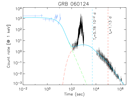
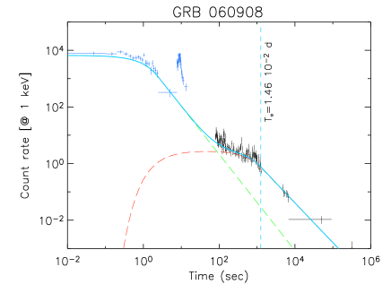
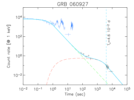
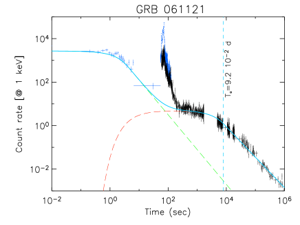
Figure 1: The early BAT and late XRT light curves of GRB 060124, GRB 060908, GRB 060927 and GRB 061121 modelled with the function proposed by W07. The two model components are shown by the long–dashed lines while their sum is shown by the solid line. The fits were performed excluding the flares of the light curves. The long dashed vertical lines show the $T_{\rm a}$ in each light curve (for GRB 060124 we also report the jet break time found in the optical light curve – see text).

3 Analysis and results

First we study the Ghirlanda like correlation and the Liang & Zhang like correlation defined using $T_{\rm a}$ in place of $t_{\rm jet}$. We use the formalism defined in N06 where, for a generic time break $t_{\rm break}$, the jet opening angle is defined as:

$$\theta = 0.161\left({t_{\rm break}\over 1+z}\right)^{3/8}\left({n\,\eta_{\gamma}\over E_{\rm\gamma,iso,52}}\right)^{1/8}\,\,\,\,\,\,\,{\rm[HM]}$$

$$\theta = 0.2016\,\left({t_{\rm break}\over 1+z}\right)^{1/4}\left({\eta_{\gamma}\ A_{*}\over E_{\rm\gamma,iso,52}}\right)^{1/4}\,\,\,{\rm[WM]}$$ (1)

where $n$ represents the circumburst density in the homogeneous case (HM) and $A_{*}$ is the normalisation of the wind (WM) density profile ($n(r)\propto A_{*}r^{-2}$ – see N06 for more details). Here $\eta_{\gamma}$ is the radiative efficiency of the prompt phase assumed to be 0.2 for all bursts.

In both cases of Eq. 1, it is necessary to know the isotropic bolometric rest frame equivalent energy $E_{\rm\gamma,iso}$. This is

$$E_{\rm\gamma,iso}\,=\,{4\pi d^{2}_{L}S_{\gamma}k\over 1+z}$$ (2)

where $d_{L}$ is the luminosity distance, $S_{\gamma}$ is the $\gamma$–ray fluence in the observed energy band, $k$ is the bolometric correction factor needed to find the energy emitted in a fixed energy range (here, 1–10⁴ keV) in the rest frame of the source. For most pre–Swift bursts the spectrum is fitted with the Band function (Band et al. 1993) composed by two smoothly joint power laws. On the other hand, several Swift bursts, due to the narrow energy range of the BAT instrument (15–150 keV), have a spectrum best fitted with a cutoff–power law model. As discussed in Firmani et al. (2006), in these cases the extrapolation of the cutoff–power law model up to 10⁴ keV may considerably underestimate the energy, if the spectrum is, instead, a Band function. To account for this limitation of the spectral fits in the Swift era, the value of $E_{\rm\gamma,iso}$ reported in Tab. 1 is an average between the value derived with the cutoff–power law model and that derived assuming a Band model with high energy photon index $\beta=-2.3$ (see also G07).

3.1 Correlation analysis

For the 23 GRBs of Tab. 1 we computed the angle $\theta_{\rm j,a}$, where the subscript “a” means that the angle has been estimated using $T_{\rm a}$ as a jet break time, and the collimation corrected energy $E_{\rm\gamma,a}$ in both the WM and HM case. The density in the homogeneous case is known only for some GRBs and for the others we take the value $n=3\pm 2.76$; the density in the wind case is assumed equal for all GRBs and without error (see N06 and G07 for details).

We report also the correlation defined with the jet break time $t_{\rm jet}$ and recently updated with the Swift bursts in G07. Here we use the sample of G07 (Tab. 1 in that paper) excluding bursts with only a lower limit on $t_{\rm jet}$. For comparison we also recomputed the $E_{\rm p}-E_{\rm\gamma,iso}$ (Amati) correlation with the sample of 40 GRBs.

The fit is performed using the routine fitexy (Press et al. 1999) which weights for the errors on the involved variables. All the fit results can be expressed in the synthetic form:

$$\left({E_{\rm p}\over 100\,{\rm keV}}\right)\,=\,(K\pm\sigma_{\rm K})\,\left({E_{\rm\gamma,a}\over E_{\rm bar}}\right)^{s\pm\sigma_{\rm s}}$$ (3)

where $E_{\rm\gamma,a}$ must be replaced by $E_{\gamma}$ or $E_{\rm\gamma,iso}$ according to the correlation considered. Here $E_{\rm bar}$ represents the barycentre of the energy values of the sample considered.

The three correlations are shown in Fig. 2 (homogeneous case) and in Fig. 3 (wind case), and the fit results are listed in Tab. 2. For every correlation we report also the reduced $\chi^{2}$ and the 1$\sigma$ scatter of the data points around the best fit line, modelled with a gaussian distribution.

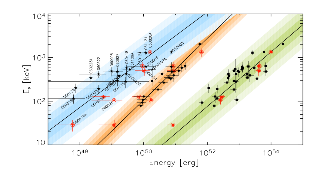
Figure 2: Homogeneous circumburst medium. From right to left we show the $E_{\rm p}-E_{\rm\gamma,iso}$ correlation (filled squares – 40 GRBs), the $E_{\rm p}-E_{\gamma}$ correlation (filled circles – 23 bursts from G07) and the $E_{\rm p}-E_{\rm\gamma,a}$ correlation (filled stars – 23 GRBs of Tab. 1). The shaded regions (for the three correlations) represent the 1, 2, 3$\sigma$ scatter of the data points (computed perpendicular) with respect to the best fitted correlation (solid lines). Circled points (on the three correlations) represent the 6 Swift bursts for which both $T_{\rm a}$ and $t_{\rm jet}$ are known.

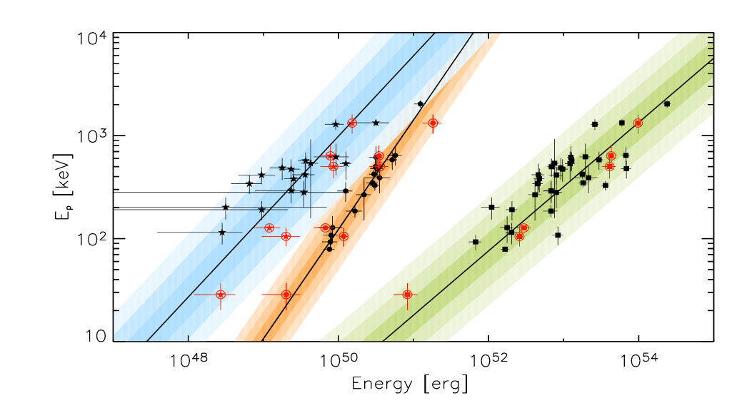
Figure 3: Wind circumburst medium. Symbols as in Fig.2

Correlation	Density	N	$K$	$s$	$E_{\rm bar}$	$\chi^{2}_{\rm r}$	Scatter
	profile		($\sigma_{\rm K}$)	($\sigma_{\rm s})$	(erg)
$E_{\rm p}-E_{\rm\gamma,a}$	homog.	23	4.71 (0.37)	0.55 (0.05)	$3.11\times 10^{49}$	1.95 (21 d.o.f.)	0.16
$E_{\rm p}-E_{\rm\gamma,a}$	wind	23	4.95 (0.38)	0.78 (0.07)	$4.14\times 10^{49}$	1.95 (21 d.o.f.)	0.16
$E_{\rm p}-E_{\gamma}$	homog	23	2.89 (0.16)	0.71 (0.04)	$4.14\times 10^{50}$	1.14 (21 d.o.f.)	0.09
$E_{\rm p}-E_{\gamma}$	wind	23	3.21 (0.17)	1.06 (0.07)	$2.47\times 10^{50}$	0.91 (21 d.o.f.)	0.08
$E_{\rm p}-E_{\rm\gamma,iso}$	——	40	3.77 (0.11)	0.62 (0.02)	$1.31\times 10^{53}$	5.70 (38 d.o.f.)	0.16
$E_{\rm p}-E_{\rm\gamma,iso}$	——	23	4.83 (0.21)	0.65 (0.03)	$1.22\times 10^{53}$	2.89 (21 d.o.f.)	0.15

Table 2: Best fit results of the correlations involving the rest frame peak energy and the collimation corrected energy computed either using $T_{\rm a}$ as a jet break time and the real jet break time $t_{\rm jet}$. We also report the Amati correlation for the considered 40 GRBs and for the 23 defining also the $E_{\rm p}-E_{\rm\gamma,a}$ correlation. The collimation corrected correlations are reported for both the homogeneous and wind medium scenario. $K$ and $s$ represent the normalisation and slope, respectively, of the best fit correlation (see Eq. 3). The 1$\sigma$ scatter of the data points around the best fit correlation is also reported.

From the comparison of the results reported in Tab. 2 and in Figs. 2 and 3 we note:

1. the correlation $E_{\rm p}-E_{\rm\gamma,a}$ derived using $T_{\rm a}$ as a jet break time is not parallel to the $E_{\rm p}-E_{\gamma}$ correlation (derived using $t_{\rm jet}$). In particular, independently from the specific density profile considered, the $E_{\rm p}-E_{\rm\gamma,a}$ correlation is much flatter than the $E_{\rm p}-E_{\gamma}$ correlation and in the homogeneous case it is even slightly flatter than the Amati correlation. By reconstructing the sample of W07 (through the quoted GCNs and the values given in that paper), and analyzing this smaller sample, we indeed obtain a $E_{\rm p}-E_{\rm\gamma,a}$ correlation parallel to the $E_{\rm p}-E_{\gamma}$ one, although not as tight. It is the inclusion of the additional GRBs that changes the slope of $E_{\rm p}-E_{\rm\gamma,a}$ correlation and further increases its scatter. Also the 6 GRBs with both $T_{\rm a}$ and $t_{\rm jet}$ (encircled symbols) seem to define a $E_{\rm p}-E_{\rm\gamma,a}$ parallel to the $E_{\rm p}-E_{\gamma}$ correlation, and this issue will be discussed in Sec. 3.2.

2. the fit of the $E_{\rm p}-E_{\rm\gamma,a}$ correlation (in terms of $\chi^{2}$) is significantly worse than that of the $E_{\rm p}-E_{\gamma}$ correlation, which, instead, is statistically acceptable;

3. the $E_{\rm p}-E_{\rm\gamma,a}$ correlation has a scatter which is a factor 2 larger than that of the $E_{\rm p}-E_{\gamma}$ correlation and is similar to that of the Amati correlation.

Item (i) suggests that the relation between $t_{\rm jet}$ and $T_{\rm a}$, if any, is not trivial (i.e. $t_{\rm jet}$ is not simply proportional to $T_{\rm a}$ as suggested by W07). The large scatter of the $E_{\rm p}-E_{\rm\gamma,a}$ correlation, which is comparable to that of the $E_{\rm p}-E_{\rm\gamma,iso}$ correlation, raises the question whether the new added variable $T_{\rm a}$ can be treated as a jet break time or not. If not, we are still left with the possibility that a completely phenomenological correlation between $E_{\rm p}$ and $E_{\rm\gamma,iso}$ and $T^{\prime}_{\rm a}$ exists (where $T^{\prime}_{\rm a}$ is the time in the source rest frame). This possibility will be explored in the next section.

3.2 The $E_{\rm p}$–$E_{\rm\gamma,iso}$–$T^{\prime}_{\rm a}$ correlation

In this section we study the $E_{\rm p}$–$E_{\rm\gamma,iso}$–$T^{\prime}_{\rm a}$ correlation. First we fit the multi–variable correlation with the 23 GRBs of Tab. 1 through a least–square method without considering the errors on the three variables. The result is:

$$E_{\rm\gamma,iso,52}\, = (7.29\pm 0.89)\,\left(E_{\rm p}\over 357\,{\rm keV}\right)^{1.5\pm 0.1}\,\times$$ (4)

$$\left(T^{\prime}_{\rm a}\over 0.012\,{\rm s}\right)^{0.06\pm 0.59}.$$

Note that the exponent of $T^{\prime}_{\rm a}$ is very close to zero and this implies that $T^{\prime}_{\rm a}$ does not reduce the scatter of the $E_{\rm p}-E_{\rm\gamma,iso}$ correlation. Indeed, the above result is almost identical to the $E_{\rm p}-E_{\rm\gamma,iso}$ correlation defined by the 23 GRBs reported in Tab. 1 (see also the last row of Tab. 2).

For consistency with the fits reported in the previous sections we also fitted the $E_{\rm p}$–$E_{\rm\gamma,iso}$–$T^{\prime}_{\rm a}$ correlation by weighting for the errors on the three variables. In this case we find a different result:

$$E_{\rm\gamma,iso,52}\, = (13.8\pm 2.0)\,\left(E_{\rm p}\over 513\,{\rm keV}\right)^{2.18\pm 0.53}\,\times$$ (5)

$$\left(T^{\prime}_{\rm a}\over 0.0173\,{\rm s}\right)^{-0.67\pm 0.43}.$$

with a reduced $\chi^{2}=2.28$ (20 dof). The reason for the difference with Eq. 4 lies in the errors on $T^{\prime}_{\rm a}$, which are particularly large (see Tab. 1). To prove it, we have reduced the errors on $T^{\prime}_{\rm a}$ by a factor 1.5 and recovered the result of the fit with a simple linear regression analysis (Eq. 4).

In Fig. 4 we compare the scatter of the data points around the $E_{\rm p}-E_{\rm\gamma,iso}$ correlation (defined by the 23 GRBs of Tab. 1) with the scatter of the data points around the best fit plane of Eq. 5 (i.e. obtained by weigthing for the errors). We note that the scatter of the data points in the $E_{\rm p}$–$E_{\rm\gamma,iso}$–$T^{\prime}_{\rm a}$ plane is comparable to the scatter of the data points in the $E_{\rm p}$–$E_{\rm\gamma,iso}$ plane. This suggests that, although in Eq. 5 (found by weighting for the errors) the exponent of $T^{\prime}_{\rm a}$ is different from zero, the scatter of the data points is not improved with respect to the $E_{\rm p}-E_{\rm\gamma,iso}$ correlation. We conclude that it is Eq. 4 which better represents the best fit to the data.

Figure 4: Scatter distribution of the 23 GRBs of Tab. 1 around the best fit $E_{\rm p}-E_{\rm\gamma,iso}$ correlation (top histogram) compared with the scatter of the same points around the best fit plane of the $E_{\rm p}$–$E_{\rm\gamma,iso}$–$T^{\prime}_{\rm a}$ correlation defined by Eq. 5 (bottom histogram). One can see that the scatter of the $E_{\rm p}$–$E_{\rm\gamma,iso}$–$T^{\prime}_{\rm a}$ correlation is similar (if not larger) than the scatter of the $E_{\rm p}-E_{\rm\gamma,iso}$ correlation.

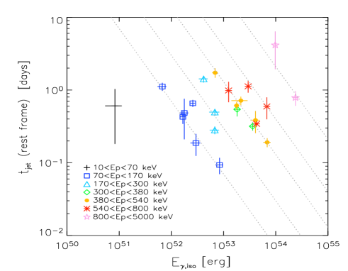
Figure 5: The time $t_{\rm jet}$ as a function of $E_{\rm\gamma,iso}$ for the burst of the G07 sample. Bursts with different peak energy ranges (as labelled) are shown with different symbols. The dotted lines indicate $t_{\rm jet}$$\propto E_{\rm\gamma,iso}^{-1}$, with different normalizations, to illustrate that bursts with the same $E_{\rm p}$ do follow this law.

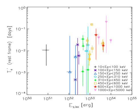
Figure 6: The time $T^{\prime}_{\rm a}$ vs $E_{\rm\gamma,iso}$ for the burst of this paper (Tab. 1). As in Fig. 5 we use different symbols for bursts with $E_{\rm p}$ in different ranges.

This would be sufficient to demonstrate that $T_{\rm a}$ does not help to define a tighter correlation between the isotropic energy and $E_{\rm p}$. To further demonstrate this point, we directly study the relation between $T_{\rm a}$ and $E_{\rm\gamma,iso}$, comparing it with the corresponding relation between $t_{\rm jet}$ and $E_{\rm\gamma,iso}$.

Consider bursts with the same $E_{\rm p}$. For these the existence of the empirical Liang & Zhang correlation implies that $E_{\rm\gamma,iso}$$\propto{t^{\prime}_{\rm jet}}^{-1}$. This is proved by the data: in Fig. 5 we show the anticorrelation between $t_{\rm jet}$ (rest frame) and $E_{\rm\gamma,iso}$ for the sample of 23 GRB by considering bursts with similar $E_{\rm p}$ (corresponding to the different symbols in Fig. 5). The $E_{\rm\gamma,iso}$$\propto{t^{\prime}_{\rm jet}}^{-1}$ relation converts in $E_{\rm\gamma,iso}$$\theta_{\rm jet}^{2}$=const (the “Frail correlation”) when using the relation between $t_{\rm jet}$ and $\theta_{\rm j}$ (Eq. 1), for both the HM and the WM cases.

Consider now Fig. 6, showing $T^{\prime}_{\rm a}$ versus $E_{\rm\gamma,iso}$: in this case $T^{\prime}_{\rm a}$ does not anticorrelate with $E_{\rm\gamma,iso}$, for constant $E_{\rm p}$. The absence of the anticorrelation translates in the impossibility to obtain a similar “Frail correlation” when using $T_{\rm a}$ as a jet angle indicator (i.e. inserting $T_{\rm a}$ instead of $t_{\rm jet}$ in Eq. 1).

3.3 The origin of the $E_{\rm p}-E_{\rm\gamma,a}$ correlation

Although $T_{\rm a}$ spans 3 orders of magnitudes, and although it is not a jet angle indicator, the $E_{\rm p}-E_{\rm\gamma,a}$ correlation exists and has a scatter comparable (or slightly larger) than the scatter of the $E_{\rm p}-E_{\rm\gamma,iso}$ correlation. What is, then, its origin?

In Eq. 1 the jet angle depends on both the break time (either $T_{\rm a}$ or $t_{\rm jet}$) but also on $E_{\gamma,\rm iso}/\eta_{\gamma}$. This term is the kinetic energy of the GRB outflow left–over after the prompt radiative phase. Since, usually, one assumes a constant value $\eta_{\gamma}=0.2$, the collimation correction depends on $E_{\rm\gamma,iso}$.

In this section we explore the role of $E_{\rm\gamma,iso}$ and $t_{\rm break}$ (either identified as $T_{\rm a}$ or $t_{\rm jet}$) in Eq. 1 in shaping the $E_{\rm p}-E_{\rm\gamma,a}$ and the $E_{\rm p}-E_{\gamma}$ correlation and their scatter.

From Eq. 1 considering only the dependencies from $E_{\rm\gamma,iso}$ and $t_{\rm break}$ we find (under the assumption of small angles):

$$\rm WM:\mbox{$E_{\gamma}$} \propto \mbox{$E_{\rm\gamma,iso}$}~{}\theta^{2}\propto\mbox{$E_{\rm\gamma,iso}$}~{}\frac{t_{\rm break}^{1/2}}{E^{1/2}_{\rm\gamma,iso}}\propto E^{1/2}_{\rm\gamma,iso}t_{\rm break}^{1/2}$$

$$\rm HM:\mbox{$E_{\gamma}$} \propto \mbox{$E_{\rm\gamma,iso}$}~{}\theta^{2}\propto\mbox{$E_{\rm\gamma,iso}$}~{}\frac{t_{\rm break}^{3/4}}{E^{1/4}_{\rm\gamma,iso}}\propto E^{3/4}_{\rm\gamma,iso}t_{\rm break}^{3/4}$$ (6)

Consider those GRBs that have the same $E_{\rm p}$, but different $E_{\rm\gamma,iso}$. Even if they have the same $t_{\rm break}$, the use of Eq. 6 implies a clustering of the corresponding collimation corrected $E_{\gamma}$: GRB with larger $E_{\rm\gamma,iso}$  would have smaller $\theta$, and therefore have a larger correction for their collimation (and vice-versa).

We calculate $\theta$ and correct for the collimation factor assuming that the break time (either $T_{\rm a}$ or $t_{\rm jet}$) is constant and equal for all bursts. The use of Eq. 6 with a fixed $t_{\rm break}$ gives $E_{\gamma}\propto E_{\gamma,\rm iso}^{1/2}$ in the WM case, and $E_{\gamma}\propto E_{\gamma,\rm iso}^{3/4}$ in the HM case. We plot $E_{\rm p}$ versus this estimate of $E_{\gamma}$ in Fig. 7 (for both the WM and HM cases). The empty star symbols define a correlation which is less scattered than the $E_{\rm p}-E_{\rm\gamma,iso}$ correlation (empty circles) in the HM and WM case (left and right panels in Fig. 7). Moreover, the scatter reduction is somewhat more significant in the WM case with respect to the HM case.

Note that this result has no physical meaning and it is only due to the fact that we plot the points in the $E_{\rm p}$-$E^{1/2}_{\rm\gamma,iso}$ plane for the WM case (or $E_{\rm p}$–$E^{3/4}_{\rm\gamma,iso}$ for the HM case) instead of in the $E_{\rm p}$–$E_{\rm\gamma,iso}$ plane. Up to this point the reduction of the scatter of the $E_{\rm p}-E_{\rm\gamma,iso}$ correlation, and the difference in the slope with respect to the Amati relation, is due to the dependence of Eq. 6 (used to derive the jet opening angle) on $E_{\rm\gamma,iso}$.

We can now see if the use of the real break time (either $T_{\rm a}$ or $t_{\rm jet}$ – upper panels and lower panels in Fig. 7, respectively) improves or not the found correlations. The results in the case of $T_{\rm a}$ are shown in the upper panels of Fig. 7 for the HM and WM case. Although a correlation between $E_{\rm p}$ and $E_{\rm\gamma,a}$ appears (filled circles), we find that the effect of $T_{\rm a}$ is to increase the scatter of the data points with respect to the same correlation defined with $T_{\rm a}$ constant. Note that the scatter of the found $E_{\rm p}-E_{\rm\gamma,a}$ correlation is not less than that of the $E_{\rm p}-E_{\rm\gamma,iso}$ correlation (both in the HM and WM case). This demonstrates that the variable $T_{\rm a}$, if treated as a jet break time to estimate the angle and derive the collimation corrected energy, leaves unaltered (or even increases) the scatter of the $E_{\rm p}-E_{\rm\gamma,iso}$ correlation. This effect is clearly shown in Fig. 7 by bursts with typical rest frame peak energy in the range 100–1000 keV which are the majority in our sample.

Figure 7: Comparison of the scatter of the $E_{\rm p}-E_{\rm\gamma,a}$ and $E_{\rm p}-E_{\gamma}$ correlations in the homogeneous (left) and wind (right) medium cases. Top panels: from right to left we report the $E_{\rm p}-E_{\rm\gamma,iso}$ correlation (empty circles), the correlation defined by assuming a constant value of $T_{\rm a}$ (for all the bursts) in computing the collimation correction (empty stars) and the correlation defined by using the measured $T_{\rm a}$ (filled circles; values of $T_{\rm a}$ reported in Tab. 1). Bottom panels: same as above but considering $t_{\rm jet}$ instead of $T_{\rm a}$.

In the bottom panels of Fig. 7 we show the results obtained with $t_{\rm jet}$. As discussed in Sec. 2, the sample of bursts used to define the $E_{\rm p}-E_{\gamma}$ correlation only marginally overlaps to that used to define the $E_{\rm p}-E_{\rm\gamma,a}$ correlation: this is the reason why also the $E_{\rm p}-E_{\rm\gamma,iso}$ correlation in the lower and upper panels of Fig. 7 are different. If first we set $t_{\rm jet}$=constant and equal for all bursts we have, as before, a reduction (empty stars) of the scatter of the $E_{\rm p}-E_{\rm\gamma,iso}$ correlation (empty circles). But now, if we assign to each GRB in our sample its $t_{\rm jet}$ found from the optical light curve, we see that the scatter of the data points is further reduced (note in particular this effect in peak energy range 500–1000 keV).

From these results we conclude that:

• the dependence of the jet angle on $E_{\rm\gamma,iso}$ reduces the scatter of the $E_{\rm p}-E_{\rm\gamma,iso}$ correlation;

• the use of the time $T_{\rm a}$  which marks the end of the plateau phase in the X–ray light curves, increases the scatter of the correlation found assuming a constant $T_{\rm a}$. This effect, counterbalanced by the previous one, makes the scatter of the $E_{\rm p}-E_{\rm\gamma,a}$ correlation similar to the scatter of the $E_{\rm p}-E_{\rm\gamma,iso}$ correlation;

• the (albeit weak) positive correlation between $T_{\rm a}$ and $E_{\rm\gamma,iso}$ (see Fig. 6), makes the slope of the $E_{\rm p}-E_{\rm\gamma,a}$ correlation to differ somewhat from the slope of the correlation found with $T_{\rm a}$ constant;

• the small dispersion of the Ghirlanda relation is due not only to the presence of $E_{\rm\gamma,iso}$ in the equation for the angle, but also to the jet break time $t_{\rm jet}$.

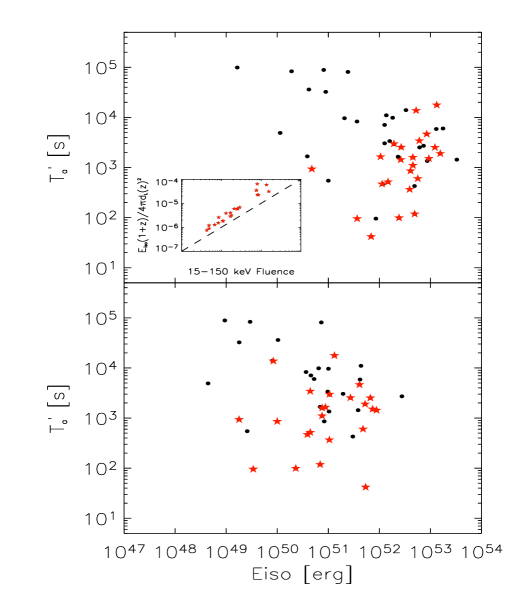
Figure 8: Top panel: the time $T^{\prime}_{\rm a}$ as a function of the isotropic energy of the prompt emission $E_{\rm\gamma,iso}$ calculated in the 15–150 keV energy range, without including any bolometric and $k$–correction for all bursts with measured redshift (circles) and for those which also have a measured $E_{\rm p}$ (stars). The insert shows the bolometric fluence vs the 15–150 keV fluence, to show that the two are proportional. Bursts in the insert are the ones in Tab. 1. Bottom panel: the time $T^{\prime}_{\rm a}$ as a function of the energy emitted in the plateau phase, in the 0.3–10 keV energy range. The fluences of the plateau phase have been taken from W07. Symbols as above.

4 Summary and discussion

We have analyzed in detail the correlation found by W07 between $E_{\rm p}$ and the collimation corrected energy $E_{\rm\gamma,a}$, found using $T_{\rm a}$ as a jet break. Our sample (of 23 objects) is larger than what used by W07, because we could add some GRB occurred after August 2006, and some other bursts for which we could find the value of $E_{\rm p}$. We find that $E_{\rm p}$ and $E_{\rm\gamma,a}$ correlate, by we also find that this correlation is weaker, and has a different slope, than the $E_{\rm p}-E_{\gamma}$ one.

Investigating further, we have also shown that the $E_{\rm p}-E_{\rm\gamma,a}$ correlation is entirely a consequence of the existence of the $E_{\rm p}-E_{\rm\gamma,iso}$ (Amati) correlation, coupled with the fact that the opening angle $\theta_{\rm j}$ depends on $E_{\rm\gamma,iso}$. This is why one finds a correlation which is narrower than the Amati one even using the same $T_{\rm a}$ for all bursts: in this case the found correlation is even better than the one obtained introducing the real $T_{\rm a}$. This demonstrates that $T_{\rm a}$ does not play any role in the $E_{\rm p}-E_{\rm\gamma,a}$ correlation: it is even worsening it.

We have then made the very same test to the $E_{\rm p}-E_{\gamma}$ (Ghirlanda) correlation, and found that in this case the use of the “real” $t_{\rm jet}$ improves the correlation, decreases the scatter and slightly changes the slope of the correlation, with respect to the one obtained using a fixed $t_{\rm jet}$.

All these results are fully confirmed by analyzing the $E_{\rm p}$–$E_{\rm\gamma,iso}$–$T^{\prime}_{\rm a}$ correlation, and comparing it to the Liang & Zhang correlation (which uses $t_{\rm jet}$ instead of $T_{\rm a}$). Again, all evidence is towards $T^{\prime}_{\rm a}$ playing no role: the found $E_{\rm p}$–$E_{\rm\gamma,iso}$–$T^{\prime}_{\rm a}$ correlation has a similar (if not larger) scatter than the $E_{\rm p}-E_{\rm\gamma,iso}$ correlation.

We conclude that the time $T_{\rm a}$ at which the plateau of the X–ray light curve ends is not an important parameter for defining the spectral–energy correlations. As a consequence, it is not a jet angle indicator. Instead, we confirm that $t_{\rm jet}$ is likely to measure the jet opening angle, since it passed our simple test to see if it helps or not to strengthen the correlation between $E_{\rm p}$ and the collimation corrected energy derived using a fixed value of $t_{\rm jet}$ for all bursts.

We note a weak correlation between $T^{\prime}_{\rm a}$ and $E_{\rm\gamma,iso}$ when considering the 23 GRBs in our sample (see Fig. 6, probability of chance correlation equal to $4\times 10^{-3}$, according to the Spearman rank correlation), which however disappears when considering the entire sample of GRBs of known redshifts and $T^{\prime}_{\rm a}$ (and relaxing the requirement to have also $E_{\rm p}$ known, see Fig. 8). Therefore we can also conclude that $T^{\prime}_{\rm a}$ is not related to $E_{\rm\gamma,iso}$, differently from $t_{\rm jet}$ which is instead anti–correlated with $E_{\rm\gamma,iso}$ when considering GRBs of similar $E_{\rm p}$. Note that, for a distribution of $T^{\prime}_{\rm a}$ not correlated (or anti–correlated) with $E_{\rm\gamma,iso}$, the resulting $E_{\rm p}-E_{\rm\gamma,a}$ correlation should become parallel to the one obtained fixing $T_{\rm a}$ to a constant value. We therefore predict that, for larger samples of GRBs with known redshift, $T_{\rm a}$ and $E_{\rm p}$, the $E_{\rm p}-E_{\rm\gamma,a}$ correlation will have a slope $\approx 0.75$ ($\approx 1$) in the HM (WM) case.

Finally, there is no correlation between $T^{\prime}_{\rm a}$ and the isotropic energy (in the observed 0.3–10 keV energy range) emitted during the plateau phase (see Fig. 8).

Unfortunately, our finding that the $E_{\rm p}-E_{\rm\gamma,a}$ correlation is only a by–product of the $E_{\rm p}-E_{\rm\gamma,iso}$ (Amati) correlation is not very helpful in shedding new light on the problem of explaining why the light curve of most GRBs is characterized by the steep–flat–steep behaviour, and also why this is sometimes different by the simultaneous behavior observed in the optical band.

Recently, we (Ghisellini et al. 2007) have proposed that the X–ray light curve is produced by internal dissipation in late shells, where “late” means that the central engine continues to create relativistic shells even days after the trigger. This implies that the central engine is long lived, and that there is a sharp transition between the early phase (determining the duration of the early prompt, i.e. the time $T_{90}$), and the late phase, emitting much smaller luminosity, but for a longer time. The early phase should be characterized by a large bulk Lorentz factor $\Gamma$ of the created shells, changing erratically, while the late phase is instead characterized by shells created with $\Gamma$ decreasing monotonically. This implies that when $\Gamma>1/\theta_{\rm j}$, we see only a fraction of the emitting surface, but when $\Gamma\leq 1/\theta_{\rm j}$ we see the entire emitting surface. This means that there should be a break in the light curve when $\Gamma=1/\theta_{\rm j}$. We associate this time to $T_{\rm a}$.

According to this idea, the two times $T_{\rm a}$ and $t_{\rm jet}$ have an obvious link: both are determined by the jet opening angle $\theta_{\rm j}$. Then, why we do not observe a relation between these two times? We propose the following answer: the time $t_{\rm jet}$ is determined when the fireball made by the merged shells of the early phase, carrying a kinetic energy $E_{\rm k}$, is decelerated by the external medium. The dynamics of the process is robust, depending only on the value of the external medium density (and its profile with distance), on $E_{\rm k}$, and finally on the conservation of energy and momentum. We have the same $\Gamma(t)$ law for different GRBs, if the external medium has the same profile.

On the contrary, the law characterizing how $\Gamma$ changes as a function of time during the late prompt phase can be different from burst to burst. As far as we know, there might not be a robust analog of the conservation of energy and momentum dictating the $\Gamma(t)$ behaviour in this case. Indeed, we can have information on this law from the observed slopes of the light curve (see Ghisellini et al. 2007), and under simplifying hypotheses we can already derive that $\Gamma(t)$ is different from one bursts to another. As a consequence, there is no general formula, equal to all bursts, in which $T_{\rm a}$ can be inserted to derive the jet opening angle.

References

- [] Amati, L., Frontera, F., Tavani, M., et al. 2002, A&A, 390, 81
- [] Amati, L., 2006, MNRAS, 372, 233
- [] Band D. L., et al., 1993, ApJ, 413, 281
- [] Barbier, L., Barthelmy, S., Cummings, J., et al. 2006, GCN, 4518
- [] Bellm, E., Bandstra, M., Boggs, S., Wigger, C., Hajdas, W., Smith, D.M., & Hurley, K. 2006, GCN, 5838
- [] Blustin, A.J., Band, D., Barthelmy, S., et al. 2006, ApJ, 637, 901
- [] Burrows et al., 2005, Sci, 309, 1833
- [] Butler, N.R. & Kocevski, D., 2007, subm to ApJ (astro–ph/0612564)
- [] Cenko, S.B., Kasliwal, M., Harrison, F.A., et al. 2006, ApJ, 652, 490
- [] Crew, G., Ricker, G., Atteia, J-L., et al. 2005, GCN, 4021
- [] Curran, P., Kann, D.A., Ferrero, P., Rol, E. & Wijers R.A.M.J., 2006, Il Nuovo Cimento C., in press (astro–ph/0611189)
- [] Firmani et al., 2006, MNRAS, 370, 185
- [] Frail D. et al., 2001, ApJ, 562, L55
- [] Gehrels, N., Chincarini, G., Giommi P., et al., 2004, ApJ, 611, 1005
- [] Ghirlanda, G., Ghisellini, G. & Lazzati, D., 2004, ApJ, 616, 331 (GGL04)
- [] Ghirlanda, G., Nava, L., Ghisellini, G. & Firmani, C., 2007, A&A subm (G07)
- [] Ghisellini, G., Ghirlanda, G., Nava, L. & Firmani, C., 2007, ApJ Lett. subm. (astro–ph/0701430)
- [] Golenetskii, S., Aptekar, R., Mazets, E., Pal’shin, V., Frederiks, D., & Cline, T. 2005a, GCN, 3179
- [] Golenetskii, S., Aptekar, R., Mazets, E., Pal’shin, V., Frederiks, D., & Cline, T. 2005b, GCN, 3518
- [] Golenetskii, S., Aptekar, R., Mazets, E., Pal’shin, V., Frederiks, D., & Cline, T. 2005c, GCN, 4238
- [] Golenetskii, S., Aptekar, R., Mazets, E., Pal’shin, V., Frederiks, D., Ulanov, M., & Cline, T. 2006a, GCN, 4989
- [] Golenetskii, S., Aptekar, R., Mazets, E., Pal’shin, V., Frederiks, D., & Cline, T. 2006b, GCN, 5837
- [] Liang, E. & Zhang, B., 2005, ApJ, 633, L611
- [] Kumar, P. & Panaitescu, A., 2000, ApJ, 647, 1213
- [] Nava, L., Ghisellini, G., Ghirlanda, G., Tavecchio, F. & Firmani, C., 2006, A&A, 450, 471 (N06)
- [] Nousek J., et al., 2006, ApJ, 642, 389
- [] O’Brien et al., 2006,, ApJ, 647, 1213
- [] Palmer, D., Barbier, L., Barthelmy, S., et al. 2006, GCN, 4697
- [] Perri, M., Giommi, P., Capalbi, M., et al. 2005, A&A, 442, L1
- [] Press, W.H. et al. 1999, Numerical Recipes in C, Cambridge University Press, 661
- [] Rees, M.J. & Meszaros, P., 1992, MNRAS 258, L41
- [] Rhoads J., 1997, ApJ, 487, L1
- [] Romano, P., Campana, S., Chincarini, G., et al. 2006, A&A, 456, 917
- [] Sato, G., Yamazaki, R., Ioka, K., et al. 2006, astro-ph/0611148, accepted for publication in ApJ
- [] Schaefer, B.E. 2007, ApJ, in press (astro–ph/0612285)
- [] Stamatikos, M., Barbier, L., Barthelmy, S., et al. 2006a, GCN, 5289
- [] Stamatikos, M., Barbier, L., Barthelmy, S., et al. 2006b, GCN, 5639
- [] Willingale, R., et al., 2007, subm to ApJ (W07) (astro–ph/0612031)