On the structure of the interstellar atomic gas

Abstract

The interstellar atomic hydrogen is known to be a 2-phase medium in which turbulence plays an important rôle. Here we present high resolution numerical simulations describing the gas from tens of parsec down to hundreds of AU. This high resolution allows to probe numerically, the small scale structures which naturally arises from the turbulence and the 2-phase physics.

¹ Laboratoire de radioastronomie millimétrique, UMR 8112 du CNRS,
École normale supérieure et Observatoire de Paris, 24 rue Lhomond,
75231 Paris cedex 05, France
² Service d’Astrophysique, CEA/DSM/DAPNIA/SAp, C. E. Saclay,
F-91191 Gif-sur-Yvette Cedex

1. Introduction

The interstellar atomic hydrogen (HI) has been extensively observed over the years (e.g. Kulkarni & Heiles 1987, Dickey & Lockmann 1990, Joncas et al. 1992, Heiles & Troland 2003, 2005, Miville-Deschênes et al. 2003). Although HI has also received a lot of attention from the theoretical point of view (Field 1965, Field et al. 1969, Wolfire et al. 1995) and in spite of the early recognition that HI is a turbulent medium (e.g. Heiles & Troland 2005), it is only recently that the dynamical properties of HI have been investigated mainly because of the large dynamical range which is necessary to treat the problem.

Here we present high resolution numerical simulations aiming to describe a turbulent atomic hydrogen flow from scales of few tens of parsec down to scales of few hundreds of AU. Such simulations have been performed with less spatial resolution by Gazol et al. (2001), Audit & Hennebelle (2005), Heitsch et al. (2005, 2006), Vázquez-Semadeni et al. (2006). In section 2, we first present the equations of the problem, we then discuss the different spatial scales important in this problem as well as the numerical setup. In section 3, we present our results. Section 4 concludes the paper.

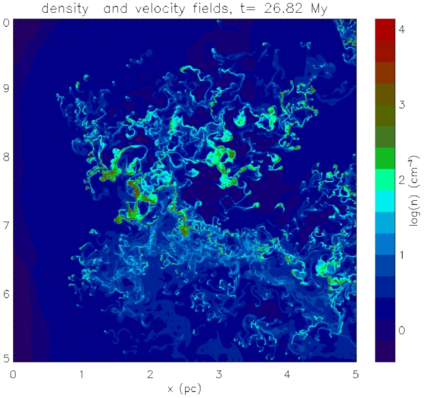
Figure 1.: Density and velocity fields at time 26.82 Myrs.

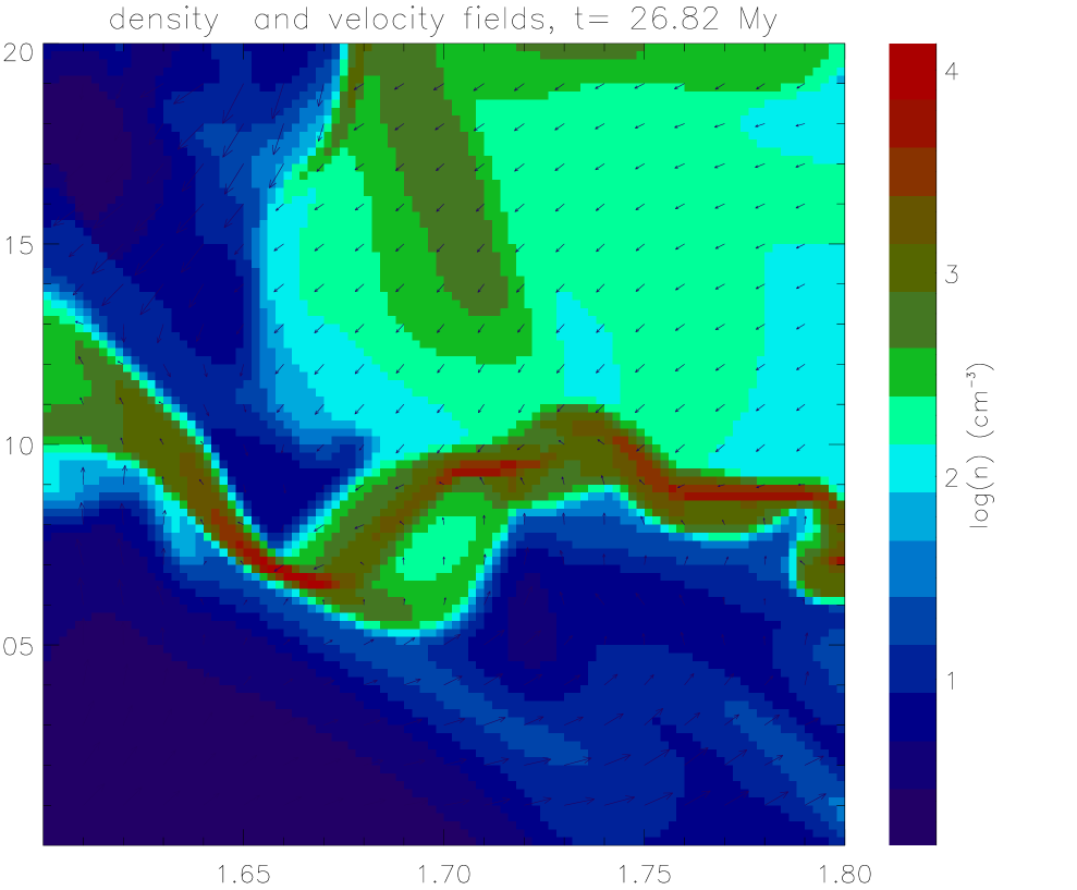
Figure 2.: Spatial zoom of Fig. 1.

Figure 3.: One dimensional cut along y-axis of the field displayed in Fig. 1. Density, temperature, Pressure and velocity fields are displayed.

2. Equations, Spatial scales and numerical Setup

We consider the usual fluid equations for a radiatively cooling gas including thermal conductivity namely,

$$\partial_{t}\rho \ +\nabla.[\rho u] = 0,$$ (1)

$$\partial_{t}\rho u \ +\nabla.[\rho u\otimes u+P] = 0,$$ (2)

$$\partial_{t}E \ +\nabla.[u(E+P)] = -{\cal L}(\rho,T)+\nabla(\kappa(T)\nabla T).$$ (3)

$\rho$ is the mass density, $u$ the velocity, $P$ the pressure, $E$ the total energy and ${\cal L}$ the cooling function which includes Lyman-$\alpha$ $C^{+}$ and $O$ line cooling and grains photoelectric heating. The gas is assumed to be a perfect gas with $\gamma=5/3$ and with a mean molecular weight $\mu=1.4m_{H}$, where $m_{H}$ is the mass of the proton. $\kappa$ is the thermal conductivity and is given by $\kappa(T)=\gamma C_{v}\eta(T)$ where $C_{v}=k_{b}/m_{H}/(\gamma-1)$, $\eta=5.7\times 10^{-5}$ (T/1 K)^1/2 g cm^-1 s^-1 and $k_{b}$ is the Boltzman constant. Various physical lengths appear to play an important rôle for the structure and the dynamics of this 2-phase flow.

The Field length (Field 1965, Koyama & Inutsuka 2004) is the length at which thermal diffusivity becomes comparable to the heating and cooling term. Its typical value is about 0.1 pc in the WNM and about $10^{-3}$ pc in the CNM. The Field length is also the typical scale of the thermal fronts which connect the cold and warm phases.

Three scales whose origin is due to dynamical processes have to be distinguished. The first scale is the cooling length of the WNM, i.e. the product of the cooling time and the sound speed within WNM, $\lambda_{\rm cool}=\tau_{\rm cool}\times C_{\rm s,WNM}$. This scale is about 10 pc and corresponds to the typical length at which WNM is non linearly unstable and can be dynamically triggered by a compression into the unstable regime (Hennebelle & Pérault 1999, 2000, Koyama & Inutsuka 2000).

Since the ratio between the CNM and WNM density is about hundred, the size of a CNM structure formed through the contraction of a piece of WNM of size $\lambda_{\rm cool}$, will be typically hundred time smaller (assuming a monodimensionnal compression). Therefore the size of the CNM structures is about the cooling length of WNM divided by hundred, leading to about $\lambda_{\rm cool}/100\simeq$0.1 pc.

As first pointed out by Koyama & Inutsuka (2002), the fragments of CNM have a velocity dispersion with respect to each others which is a fraction of the sound speed of the medium in which they are embedded, i.e. WNM. Since the contrast between the sound speed within the two phases is about 10, it means that CNM structures undergo collisions at Mach number, $M\simeq$ 10. If for simplicity we assume isothermality and apply simple Rankine-Hugoniot conditions, we obtain that the size of the shocked CNM structures is given by the size of the CNM structures divided by $M^{2}$ which is about $10^{-3}$ pc.

As clearly shown by these numbers, the resolution necessary to describe fairly a 2-phase fluid like the neutral atomic gas is very mandatory. We therefore choose to perform 2D numerical simulations which allow to describe much smaller scales than 3D simulations. We use 10000⁴ cells with a 20 pc size box leading to a spatial resolution of 0.002 pc.

The boundary conditions consist in an imposed converging flow at the left and right faces of amplitude $1.5\times C_{s,wnm}$ on top of which turbulent fluctuations have been superimposed. On top and bottom face outflow conditions have been setup. This means that the flow is free to escape the computational box across these 2 faces. The initial conditions are a uniform low density gas ($n\simeq 0.8$ cm^-3) at thermal equilibrium corresponding to WNM. It is worth noticing that initially no CNM is present in the computational box. The simulations are then runned until a statistically stationary state is reached. This requires typically about 5 to 10 box crossing times. At this stage the incoming flow of matter compensate on average the outgoing material.

3. Results

Figure 1 shows the density field at time 26.82 Myrs after the beginning of the calculation. At this stage the statistical properties of the flow do not evolve any more. The structure of the medium appears to be rather complex. The cold phase is very fragmented into several long living cloudlets confined by the external pressure of the WNM. This is more clearly seen in Fig. 2 and 3 in which much smaller scales are visible. The importance of the pressure confinement of the structures by the surrounding warm gas is well seen on the density peaks of Fig. 3 which, except for the notable exception of the structure located at $x\simeq 7.05$ pc, show either no correlation with the pressure or an anti-correlation. Large density fluctuations, well above the mean CNM density, can be seen. Such fluctuations are due to the collisions between the cold CNM fragments and are therefore located at the stagnation points of converging flows. This is well illustrated by the small (400-800 AU) and dense structures seen in Fig. 2 at $x\simeq 1.66,y\simeq 7.07$ pc, $x\simeq 1.72,y\simeq 7.10$ pc and $x\simeq 1.77,y\simeq 7.90$ pc for which the density reaches about 10⁴ cm^-3. The size and density of the structures is therefore comparable to the typical values of shocked CNM fragments recalled in section 2 and are reminiscent of the values inferred for the tiny small scale atomic structures (TSAS) quoted e.g. by Heiles (1997). It is therefore tempting to propose that the TSAS are naturally produced by the 2-phase nature of the flow which naturally generates high Mach collisions between cold CNM fragments. Note that the spatial resolution available in the simulation presented here, is still not sufficient to fully resolve these small structures and one expects that with higher resolution, structures with even larger densities and smaller size will be formed. As can be seen in Fig. 3 ($y\simeq 7.05$), the pressure in these objects is well correlated with the density as it is expected in a high Mach number shock. This large pressure is dynamically maintained by the ram pressure of the large scale converging flow and the life time of the shocked CNM structure is about the size of the colliding CNM clouds divided by their respective velocity. For 0.1 pc clouds endorging collisions at Mach 10, this is about 10⁴ years.

Another interesting aspect is the large number of small CNM structures seen in Fig. 1 and 3 (e.g. $x\simeq 6.67$ and $x\simeq 6.83$ pc). These structures which have a density of about 100 cm^-3 can be as small as few thousands of AU. They are reminiscent of recent observations of low column density CNM structures observed by Braun & Kanekar (2005) and Stanimirović & Heiles (2005).

Quantitative statistical characterizations of these numerical simulations, as well as more quantitative comparisons with observations, will be given in Hennebelle & Audit (2007) and Hennebelle, Audit & Miville-Deschênes (2007).

Finally we note that in order to verify that the trends inferred from these simulations is not affected qualitatively by their bidimensionality, we have performed 3D simulations with a grid of 1200³ cells. Although the resolution of these simulations is not sufficient to provide a description of the CNM structures down to the smaller scales, we have obtained similar results.

4. Conclusion

We have performed high resolution numerical simulations of a turbulent atomic gas. The resulting structure appears to be very complex. The CNM is very fragmented in long living cloudlets bounded by contact discontinuities and confined by the surrounding WNM. Small scale structures either dense (up to 10⁴ cm^-3) or having density of standard CNM, appear to form naturally as a consequence of the turbulence and the 2-phase physics. Both have physical parameters which are reminiscent with the values inferred from observations of TSAS and recently observed low column density atomic clouds.

References

- (1) Audit E., Hennebelle P., 2005, A&A 433, 1
- (2) Braun R., Kanekar N., 2005, A&A 436L, 53
- (3) Dickey J., Lockman F., 1990, ARA&A, 28, 215
- (4) Field G., 1965, ApJ 142, 531
- (5) Field G., Goldsmith D., Habing H., 1969, ApJ Lett 155, 149
- (6) Gazol A., Vázquez-Semadeni E., Sánchez-Salcedo F., Scalo J., 2001, ApJ 557, L124
- (7) Heiles C., 1997, ApJ 481, 193
- (8) Heiles C., Troland T., 2003, ApJ 586, 1067
- (9) Heiles C., Troland T., 2005, ApJ 624, 773
- (10) Heitsch F., Burkert A., Hartmann L., Slyz A., Devriendt J., 2005, ApJ 633, 113
- (11) Heitsch F., Slyz A., Devriendt J., Hartmann L., Burkert A., 2006, ApJ 648, 1052
- (12) Hennebelle P., Pérault M., 1999, A&A 351, 309
- (13) Hennebelle P., Pérault M., 2000, A&A 359, 1124
- (14) Hennebelle P., Audit E., 2007, A&A, in press, astro-ph/0612778
- (15) Hennebelle P., Audit E., Miville-Deschènes M.-A., 2007, A&A, in press, astro-ph/0612779
- (16) Koyama H., Inutsuka S., 2000, ApJ 532, 980
- (17) Koyama H., Inutsuka S., 2002, ApJ 564, L97
- (18) Koyama H., Inutsuka S., 2004, ApJ 602L, 25
- (19) Kulkarni S.R., Heiles C., 1987, Interstellar processes, ed. Hollenbach D., Thronson H. (Reidel)
- (20) Miville-Deschênes M.-A., Joncas G., Falgarone E., Boulanger F., 2003, A&A 411, 109
- (21) Stanimirović S., Heiles C., 2005, ApJ 631, 371
- (22) Vázquez-Semadeni E., Ryu D., Passot T., González R., Gazol A., 2006, ApJ 643, 245
- (23) Wolfire M.G., Hollenbach D., McKee C.F., 1995, ApJ 443, 152