Results of Monitoring the Dramatically Variable C IV Mini-BAL System in the Quasar HS 1603+3820

Abstract

We present six new and two previously published high-resolution spectra of the quasar HS 1603+3820 (${{z_{em}}}=2.542$) taken over an interval of 4.2 years (1.2 years in the quasar rest frame). The observations were made with the High-Dispersion Spectrograph on the Subaru telescope and Medium-Resolution Spectrograph on the Hobby-Eberly Telescope. The purpose was to study the narrow absorption lines (NALs). We use time variability as well as coverage fraction analysis to separate intrinsic absorption lines, which are physically related to the quasar, from intervening absorption lines. By fitting models to the line profiles, we derive the parameters of the respective absorbers as a function of time. Only the mini-BAL system at ${{z_{abs}}}\sim 2.43$ (${{v_{shift}}}\sim 9,500~{}{{{\rm km~{}s}^{-1}}}$) shows both partial coverage and time variability, although two NAL systems possibly show evidence of partial coverage. We find that all the troughs of the mini-BAL system vary in concert and its total equivalent width variations resemble those of the coverage fraction. However, no other correlations are seen between the variations of different model parameters. Thus, the observed variations cannot be reproduced by a simple change of ionization state nor by motion of a homogeneous parcel of gas across the cylinder of sight. We propose that the observed variations are a result of rapid continuum fluctuations, coupled with coverage fraction fluctuations caused by a clumpy screen of variable optical depth located between the continuum source and the mini-BAL gas. An alternative explanation is that the observed partial coverage signature is the result of scattering of continuum photons around the absorber, thus the equivalent width of the mini-BAL can vary as the intensity of the scattered continuum changes.

1 INTRODUCTION

Quasars have been used as background sources to study the gaseous phases of a variety of objects that are located along our sight-lines to them. These objects include not only intervening absorbers such as intervening galaxies, the intergalactic medium (IGM), clouds in the halo of the Milky Way, and the host galaxies of the quasars themselves, but also intrinsic absorbers that are physically associated with the quasar central engines. One of the most promising candidates for the intrinsic absorbers are outflowing winds from the quasars that could be accelerated by radiation pressure from the accretion disk (Murray et al. 1995; Arav et al. 1995; Proga et al. 2000) or by magnetocentrifugal forces (e.g., Everett 2005). Outflowing winds are important components of quasar central engines because they carry away angular momentum from the accretion disk and allow the remaining gas in the disk to accrete onto the central black hole. Quasar outflows are also important for cosmology since they deliver energy, momentum, and metals to the interstellar and intergalactic media, thus significantly affecting star formation and galaxy assembly (e.g., Granato et al. 2004; Scannapieco & Oh 2004; Springel, Di Matteo & Hernquist 2005).

Intrinsic narrow absorption lines (NALs; FWHM $\leq 500~{}{{{\rm km~{}s}^{-1}}}$) present a powerful way to determine physical parameters of the accretion disk winds. Unlike the broad absorption lines (BALs; FWHM $\geq 2,000~{}{{{\rm km~{}s}^{-1}}}$; Weymann et al. 1991) that are also associated with quasars outflows, NALs do not suffer from self-blending or from saturation, so that line parameters are more easily evaluated. BALs are thought to be associated with radiatively-driven outflows from accretion disks (e.g., Weymann et al. 1991; Becker et al. 1997), while it is difficult to separate intrinsic NALs from intervening NALs. Mini-broad absorption lines (mini-BALs) are an intermediate subclass between NALs and BALs, which are typically wider than those of NALs, but narrower than BALs. Mini-BALs have the advantages of both BALs (i.e., high probability of being intrinsic lines) and NALs (i.e., line profiles can be resolved into individual components), which make them useful targets (e.g., Churchill et al. 1999; Hamann et al. 1997a; Narayanan et al. 2004). BALs could probe the low-latitude, dense, fast portion of the wind, while the mini-BALs and NALs may probe the lower-density portion of the wind at high latitudes above the disk. Thus, the study of mini-BALs and NALs complements the study of BALs because the corresponding absorbers reside in different regions of the outflow and allow us to sample different sets of physical conditions.

To isolate intrinsic NALs, two tests are commonly used: (i) partial coverage, i.e., trough dilution by un-occulted light (e.g., Hamann et al. 1997b; Barlow & Sargent 1997; Ganguly et al. 1999), and (ii) variability of the absorption profiles within a few years in the quasar rest frames (e.g., Hamann et al. 1997a; Narayanan et al. 2004; Wise et al. 2004). These effects occur for intrinsic absorbers that are very compact and very dense compared to intervening absorbers. The fraction of quasars that host intrinsic C IV associated NALs (NALs within 5,000 km s^-1 of the quasar emission redshifts) has been estimated to be $\sim 25$–27% at $z<2$, using the time variability technique (Narayanan et al. 2004; Wise et al. 2004), and $\sim$23% at $z\sim 2.5$, based on partial coverage analysis (Misawa et al. 2007). These signatures are a sufficient, but not a necessary, condition to demonstrate the intrinsic nature of an absorber. It is very likely that some NALs without time variability or partial coverage are also intrinsic.

Both of the above methods have been applied to BAL and mini-BAL systems. For example, partial coverage analysis has been carried out by Petitjean & Srianand (1999), Srianand & Petitjean (2000,) Yuan et al. (2002), and Ganguly et al. (2003), while time-variability has been studied by Foltz et al. (1987), Turnshek et al. (1988), Smith & Penston (1988), Barlow et al. (1992), Barlow (1993), Vilkoviskij & Irwin (2001), Ma (2002), Narayanan et al. (2004), and Lundgren et al. (2007). It is quite difficult (or almost impossible) to deblend kinematic components in those heavily blending absorption features using low/intermediate resolution spectra. However, some authors successfully deblended narrower absorption components from each other in such systems using high resolution spectra of $R>40,000$ (e.g., Yuan et al. 2002; Ganguly et al. 2003). Systematic monitoring of individual mini-BALs using high-resolution spectra taken on several epochs can potentially provide very important constraints on the properties of the absorbers. However, no such campaign has been attempted so far, to our knowledge.

The optically bright quasar HS 1603+3820 ($z_{em}$=2.542, B=15.9), first discovered in the Hamburg/CfA Bright Quasar Survey (Hagen et al. 1995; Dobrzycki et al. 1996), is known to have a large number (13) of C IV doublets at $1.965<{{z_{abs}}}<2.554$ (Dobrzycki, Engels, & Hagen 1999). Using high-resolution spectra ($R=45,000$) taken with the Subaru telescope, Misawa et al. (2003, 2005) classified all C IV doublets into 8 C IV systems, and found that only a mini-BAL system at ${{z_{abs}}}\sim 2.43$ (shift velocity, ${{v_{shift}}}=8,300$–10,600 km s^-1) shows both partial coverage and time variability in an interval of 0.36 years in the quasar rest frame. Based on these results, Misawa et al. (2005) placed constraints (i) on the electron density ($n_{e}\geq 3.2\times 10^{4}~{}{{{\rm cm}^{-3}}}$) and the absorber’s distance from the quasar ($r\leq 6$ kpc), if a change in the ionization state causes the variability, or (ii) on the time scale for the absorber to cross the continuum source and the distance from the continuum source, if gas motion across the background UV source causes the variability. In the latter case, the crossing velocity is constrained to be $v_{cross}\geq 8,000~{}{{{\rm km~{}s}^{-1}}}$, and the distance from the continuum source, $r\leq 0.2$ pc. This is larger than the size of the continuum source, $R_{cont}\sim 0.02$ pc, but smaller than that of the BLR, $R_{BLR}$$\sim$3 pc, estimated for this quasar. On the other hand, the other C IV NALs found towards the quasar show no sign of being intrinsic. Further monitoring observations make it possible to (i) discriminate between changes in the ionization state and motion of the absorbers across the continuum source as the cause of the time variability seen in the C IV mini-BAL, and (ii) to confirm whether the other C IV NALs really show neither partial coverage nor variability.

In this paper, we present the results of monitoring HS 1603+3820 over 4.2 years (1.2 years in the quasar rest frame) based on eight spectra. Six of these spectra were taken with the High Dispersion Spectrograph (HDS; Noguchi et al. 2002) on the Subaru telescope, and two with the Medium-Resolution Spectrograph (MRS; Horner, Engel, & Ramsey, 1998) on the Hobby-Eberly Telescope (HET). The first two spectra in this time series were presented and discussed by Misawa et al (2003, 2005). With the new spectra we are able to sample the variations of the absorption lines more densely and probe the internal structure of the absorber.

In §2, we describe the observations and data reduction. The methods used for model fitting are outlined in §3. The properties of the mini-BAL and of the other NAL systems are examined in §4. The possible origins of the time variability seen in the mini-BAL system are discussed in §5, and a summary is given in §6. We adopt ${{z_{em}}}=2.542$ as the systemic redshift of the quasar, which was estimated from its narrow emission lines (Misawa et al. 2003). Time intervals between observations are given in the quasar rest frame throughout the paper, unless otherwise noted. We use a cosmology with $H_{0}$=75 km s^-1 Mpc^-1, $\Omega_{m}$=0.3, and $\Omega_{\Lambda}$=0.7.

2 OBSERVATIONS AND DATA REDUCTION

We observed HS 1603+3820 eight times over a period of 4.2 years in the observed frame, from March 2002 to May 2006. We will call the dates of these observations epoch 1 through epoch 8. Six of the observations were obtained with Subaru+HDS, using a 0$\farcs$8 or 1$\farcs$0 slit width ($R=45,000$ or 36,000), and adopting 2$\times$1 pixel binning along the slit. The red grating, with a central wavelength of 4900 Å, was used to cover as many C IV systems as possible, except for the first and the last observations that used central wavelengths of 6450 Å and 5700 Å. The other two spectra were taken with the HET+MRS. The MRS features a pair of fibers: one for the target and another for the sky, which enables us to perform sky subtraction effectively. We used a 1$\farcs$5 fiber to get $R=9,200$ spectra. A setup with a central wavelength of 7,000 Å is required for the queue observations with MRS+HET.

We reduced both the Subaru and HET data in a standard manner with the IRAF software. We used a Th-Ar spectrum for wavelength calibration. We directly fitted the continuum, which also includes substantial contributions from broad emission lines, with a third-order cubic spline function. Around heavily absorbed regions, in which direct continuum fitting is difficult, we used different techniques for the Subaru and HET spectra. For the Subaru spectra, we adopted the interpolation technique introduced in Misawa et al. (2003). Since the echelle blaze profile in HDS shows time variability during a night, we cannot directly use the instrumental blaze function as a continuum profile. In this scheme, we obtain the continuum shape by interpolating between the two echelle orders adjacent to the order of interest, after weighting flux levels based on the flat-frame spectrum [see eqn. (1) of Misawa et al. 2003]. We then divide the quasar spectrum by this interpolated continuum shape to obtain the normalized spectrum. We have verified the validity of this technique by applying it to a stellar spectrum; the continuum error is always less than 3.3%. For HET spectra, we used a blaze profile constructed from the flat field spectrum as a continuum model after multiplying it by a scaling factor to adjust its count level to that of the quasar spectrum (the scaling factor is a ratio of counts in the quasar spectrum to those in a flat spectrum for the same unabsorbed region).

An observation log is given in Table 1, in which we list the observation epoch, date of observation, relative time in the quasar rest frame, instrument, wavelength coverage, total exposure time, spectral resolving power, and signal-to-noise ratio (S/N) per pixel (after rebinning to pixel scales of 0.03 Å and 0.15 Å for Subaru and HET data, respectively). The S/N is evaluated around 5370 Å, close to the C IV mini-BAL. In Figure 1, we show a normalized spectrum, after combining 6 spectra taken with Subaru+HDS in the region redward of the Ly$\alpha$ emission line of the quasar ($\lambda>4300$ Å).

3 FITTING PROCEDURE

We used the line-fitting software package minfit (Churchill 1997; Churchill et al. 2003), with which we can fit absorption profiles with four free parameters: redshift ($z$), column density ($\log\;N$), Doppler parameter ($b$), and coverage fraction ($C_{f}$). Here, the coverage fraction is the fraction of the background continuum source and the broad-emission line region that is covered by the intrinsic absorber. The coverage fraction can be systematically evaluated in an unbiased manner by considering the optical depth ratio of resonant, rest-frame UV doublets of Lithium-like species (e.g., C IV, N V, and Si IV), namely,

$$C_{f}=\frac{(R_{r}-1)^{2}}{1+R_{b}-2R_{r}}\;,$$ (1)

where $R_{b}$ and $R_{r}$ are the residual fluxes of the blue and red members of the doublets in the continuum normalized spectrum (Hamann et al. 1997b; Barlow & Sargent 1997; Crenshaw et al. 1999). A $C_{f}$ value less than unity signifies that a portion of the background source is not occulted by the absorber. This, in turn, means the doublet is probably produced by an intrinsic absorber (e.g., Wampler et al. 1995; Barlow & Sargent 1997). We found 9 C IV systems at ${{z_{abs}}}\ =1.88$–2.55, as identified in Dobrzycki et al. (1999), but we did not detect a C IV system at ${{z_{abs}}}=2.5114$. This system was probably a false detection (Dobrzycki 2005; private communication). Among the 9 C IV systems, only the system at ${{z_{abs}}}=2.42$–2.45 is classified as a mini-BAL system, because its line width is larger than 500 km s^-1.

We carried out model fits to all C IV systems in the same manner as in our previous paper (Misawa et al. 2005), except for the mini-BAL. Misawa et al. (2005) performed a manual Voigt profile fit to the mini-BAL, because self-blending (blending of the blue and red members of the doublet) occurs in this system. In its original form, the minfit code was not able to handle such self-blended regions. The code was originally written for narrow absorption lines, thus it fitted the models to the blue and red members of doublets separately. This procedure overproduced the residual intensity at the self-blending regions because it added contributions from two components. To avoid this problem, we revised the code so as to fit models to the blue and red members of doublets simultaneously, i.e., by multiplying the contributions from the two doublet members. In this paper, we fit the observed mini-BALs automatically using this improved minfit.

As in Misawa et al. (2005), we fitted only the first (bluest) two C IV kinematic components in the system, at $\lambda_{obs}=5284$–5318 Å, because the other components are so heavily blended with each other that we cannot separate them, even with the improved minfit (i.e., minfit gives multiple solutions). At first, we remove the contamination from Si II $\lambda$1527 in System B, at $\lambda=5303$–5318 Å. The Si II $\lambda$1527 line in the system did not show any detectable variability between the first two observations. The C IV doublets for System B show neither partial coverage nor time variability, and are consistent with it being an intervening system. Therefore, the Si II $\lambda$1527 line is also not likely to vary. Thus, we removed the contamination from Si II $\lambda$1527 by dividing the observed spectra by a model profile synthesized with the line parameters of Si II $\lambda$1527, determined from an average of the first two observations presented in Misawa et al. (2005).

After removing the narrow Si II $\lambda$1527 components, we applied the improved minfit to the spectrum using two C IV components, one narrow and one broad, as in Misawa et al. (2005). During the fitting process, we initially forced the same coverage fraction for the narrow and broad components, as in Misawa et al. (2005). In that paper we showed that, during the first two epochs of observation, this solution produced an equally good fit as solutions that allowed these coverage fractions to differ. We also considered the possibility of differing coverage fractions for the narrow and broad components in later epochs of observation.

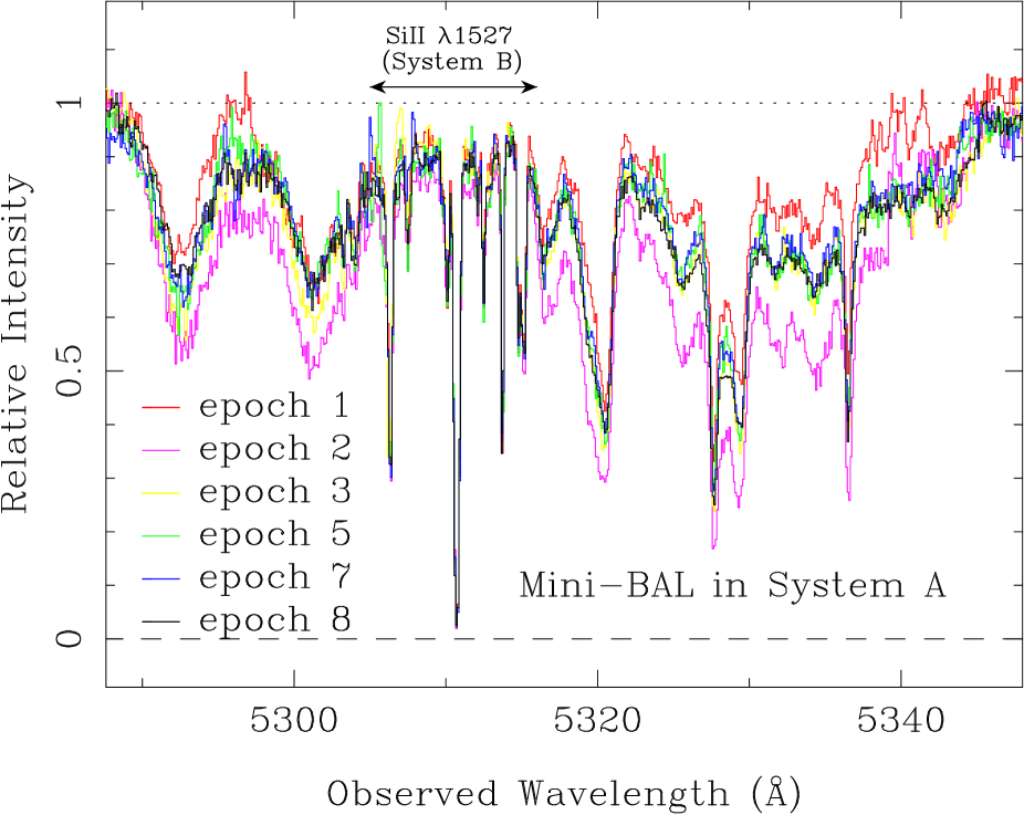
Figure 2: Normalized spectrum around the C IV mini-BAL in system A, for each Subaru+HDS observation (see electronic version in color). The absorption profile (both the broad and narrow C IV components) have obviously changed within 1 year in the quasar rest-frame. On the other hand, the Si II $\lambda$1527 line of System B did not show significant variability.

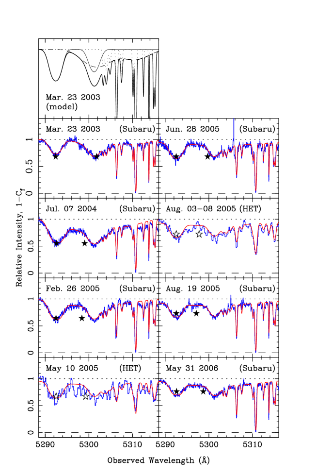
Figure 3: Observed spectra (blue histogram: see electronic version) and best-fit models (red line) of the region around C IV mini-BAL at ${{z_{abs}}}\sim 2.43$, for 8 observing epochs from March 23, 2002 to May 31, 2006. Filled stars with 1$\sigma$ errors denote the coverage fractions of narrow (left) and broad (right) components. The stars are placed at the wavelengths of the blue members of the doublet (i.e., C IV 1548). Open stars plotted in the HET spectra are coverage fractions that are interpolated from the Subaru spectra. In the top left panel, we also present models of the narrow and broad C IV components as well as the Si II $\lambda$1527 components in System B from the first observation.

Figure 2 shows 6 spectra taken with Subaru+HDS, for which we find good model fits. The fits themselves are shown in Figure 3. We cannot fit spectra obtained with HET+MRS in the same manner, because of their lower resolution and S/N. Therefore, on the HET+MRS spectra, we overplotted model profiles synthesized with parameters that are linearly interpolated between the two adjacent epochs observed with Subaru. These models provide reasonably good fits to the HET+MRS profiles. The fitting parameters for the narrow and broad C IV components, at different epochs, are summarized in Table 2. Columns (1)–(3) give the epoch number, observation date and the relative time in the quasar rest frame. Columns (4)–(8) list, for the narrow component, the shift velocity, C IV column density, C IV Doppler parameter, coverage fraction, and observed-frame equivalent width evaluated from the synthetic model spectrum. Columns (9)–(13) are the same as columns (4)–(8), but for the broad component. We confirmed that the fit parameters for the first two epochs are consistent within 1$\sigma$ errors with those presented in Misawa et al. (2005), based on a manual fitting procedure.

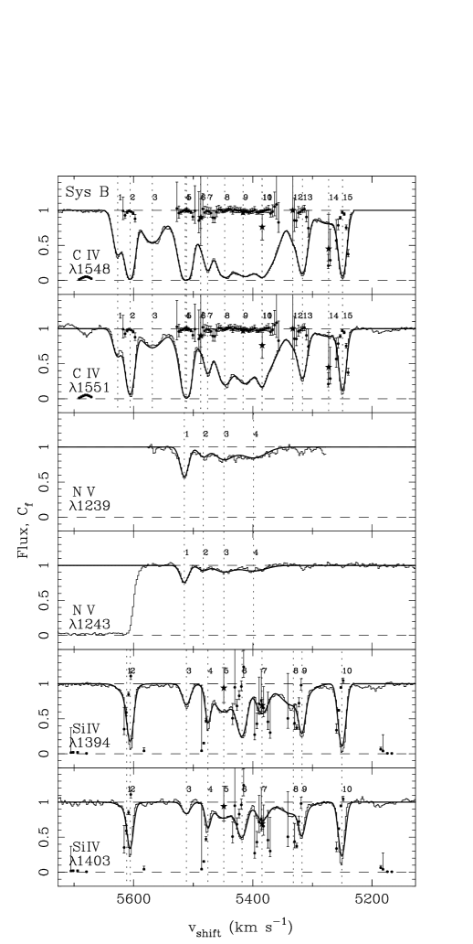
Figure 4: Velocity plots of various transitions for the 8 C IV NALs (systems B–I). Vertical dotted lines with ID numbers are the positions of absorption lines. Smooth lines are model fits using minfit. Filled stars with 1$\sigma$ error bars are coverage fractions determined by minfit. If a star is not displayed, the value of the coverage fraction is 1.0. Small dots with error bars denote the coverage fractions evaluated by the pixel-by-pixel method. The error values contain both Poisson noise and error from continuum level uncertainty.

We also applied minfit to all metal lines in the other NAL systems. Since, as described later, we did not see any remarkable variability in these NAL systems, we combined all 6 Subaru spectra to produce a final spectrum with higher S/N ($\sim$96 per pixel) before applying minfit to the NALs. The best fit parameters are summarized in Table 3. Column (1) is an identification number for the line. Columns (2) and (3) give the observed wavelength and redshift. Column (4) gives the shift velocity from the quasar systemic redshift. Columns (5) and (6) give the column density and the Doppler parameter with 1$\sigma$ errors. Column (7) reports the coverage fraction with its 1$\sigma$ error (which includes the error due to continuum level uncertainty as described below). During a fitting trial, minfit sometimes gives unphysical coverage fractions such as ${{C_{f}}}<0$ or ${{C_{f}}}\geq 1$. When this happens, the other fit parameters such as the column density and Doppler parameter have no physical meaning. These unphysical fit results could be caused by errors in the continuum fit. Misawa et al. (2005) found that the derived coverage fractions can be significantly affected by continuum level errors, especially for very weak components whose $C_{f}$ values are close to 1. Therefore, if minfit gives unphysical $C_{f}$ values for some components, we carry out the fit again for the entire line, assuming ${{C_{f}}}=1$ for those components, following Misawa et al. (2007). In this case, we do not evaluate the error in $C_{f}$. The best fit models are overlaid with the observed spectra in Figure 4(a–i).

There are also other error sources for the fit parameters, such as blending with other lines, and convolution of the true spectrum with the instrumental line spread function (LSF). Both of these are negligible if (1) the doublet is strong enough, i.e., $\log\;(N/{{{\rm cm}^{-2}}})\geq 14.0$ in the case of C IV doublets, (2) the normalized residual flux is smaller than $\sim$0.5, and (3) the line profile is much wider than the instrumental LSF (Misawa et al. 2005). Most components in our sample are broad enough compared with the LSF (corresponding to $b\sim 4~{}{{{\rm km~{}s}^{-1}}}$), and not severely blended with each other, as described in section 4.2.

4 VARIABILITY OF FIT PARAMETERS

4.1 The Mini-BAL System

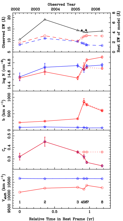
Figure 5: Variability of the C IV mini-BAL (${{z_{abs}}}\sim 2.43$) parameters over our monitoring period. From top to bottom, the frames show (1) rest frame equivalent width, (2) column densities, (3) Doppler parameters, (4) coverage fractions, and (5) shift velocities. The solid line and triangles in the top panel refer to the equivalent width of the entire mini-BAL profile (see Figures 1 and 2), while the model parameters refer to the bluest troughs (see Figure 3). The open and filled triangles in the top panel are measurements of the rest frame equivalent width, directly from the Subaru and HET data respectively. These include all C IV and Si II $\lambda$1527 components (the Si II components make only a small contribution). In all panels, the blue line and open stars refer to the narrow model component while the red line and open circles refer to the broad model component. The horizontal axis gives the observation time, both as the observed year (top label) and as the time in the quasar rest-frame, relative to the first observation (bottom label). Only the results from Subaru spectra are shown, except for the equivalent width panel, because the low-resolution and low-S/N ratio of the HET+MRS spectra prevented us from fitting models. The dotted lines in the 2nd, 3rd, and 4th panels show the best fit parameters for epoch 3 through epoch 8, assuming a constant $C_{f}$ (=0.36) for the broad component.

We previously reported that the C IV mini-BAL of System A shows trough dilution (Misawa et al. 2002), and variability within 0.36 years (Misawa et al. 2005). With the additional spectra of this paper, we follow the variability of this system for 1.2 years in the quasar rest frame, sampling it at eight epochs. N V and Ly$\alpha$ could not be identified because of heavy contamination from the Ly$\alpha$ forest. Si IV was not detected, even in our final, high-S/N spectrum. Figure 5 presents graphically the evolution of the fit parameters of the C IV mini-BAL, including (from top to bottom) the total rest frame equivalent width at $\lambda=5288$–5346 Å, the C IV column density, the Doppler parameter, the coverage fraction, and the shift velocity. We discuss each in detail below.

The total rest frame equivalent width increased by about a factor of two over a rest frame time interval of 0.36 years, and then decreased over an interval of 0.6 years. During this entire period, the general appearance of the line profile did not change significantly. Based on the results of just the first two epochs, Misawa et al. (2005) speculated that this mini-BAL may soon evolve into a BAL, with more than 10% of the flux absorbed over at least a 2,000 km s^-1 range. This idea is not confirmed by the subsequent epochs, since the mini-BAL was found to weaken. We also monitored the equivalent widths of the narrow and broad components, separately. At first, both components have almost the same equivalent width. But after epoch 3, the equivalent width of the broad component was much higher than that of narrow component.

The variability of the column density in the mini-BAL is complex. This is especially true for the broad component, which showed a large increase in column density within 0.13 years, from epoch 3 to epoch 7, as shown in Figure 5. This increase in column density was concurrent with the increase of equivalent width, as shown in the top window of the figure. One possible explanation for this dramatic increase is a change of the ionization state of the gas (Hamann et al. 1997b; Narayanan et al. 2004), which we discuss further in §5.

An interesting trend is seen in Doppler parameter variability. From epoch 3 to epoch 5 (an interval of 0.09 years in the quasar rest frame), the Doppler parameter of the broad component increased suddenly from $\sim 350~{}{{{\rm km~{}s}^{-1}}}$ to $\sim 860~{}{{{\rm km~{}s}^{-1}}}$, and then it decreased gradually. This abrupt jump is correlated with the sudden increase of the column density in the broad component, as described above. On the other hand, the narrow component did not show a significant change in Doppler parameter.

The coverage fraction (assuming it is the same for the narrow and broad components) shows a variability similar to that of the total equivalent width. After increasing to 0.45, the coverage fraction decreased to 0.24. Inspection of the separate contributions of the broad and narrow components to the total equivalent width shows that the coverage fraction evolves similarly to the equivalent width of the narrow component. If the change of coverage fraction is caused by the absorber’s motion across the background flux source, the absorber size is constrained to be smaller than the background source (about half of the background source because of the maximum $C_{f}$ value of $\sim$0.5). At the same time, the column density increased, suggesting an inhomogeneous absorber. A more detailed discussion will be presented in §5.

The column density and equivalent width of the broad component increased over the same period (epoch 3 to epoch 8) as its coverage fraction decreased. However, since we assumed that the broad and narrow components had the same coverage fractions, we must assess whether this assumption could lead to the observed trends. Specifically, we consider the effect of assuming a constant $C_{f}$ for the broad component (adopting ${{C_{f}}}=0.36$ for epoch 3 through epoch 8, and allowing the narrow component $C_{f}$ to change as before). This model, which also produced an adequate fit to the data, is illustrated with the dotted lines in the 2nd, 3rd, and 4th panels from the top of Figure 5. For this case, the column density of the broad component does not increase as rapidly, but it still does increase. The same applies for the equivalent width. Thus our conclusions regarding the evolution of the column density and equivalent width are not qualitatively changed by our assumption about the $C_{f}$ value of the broad component.

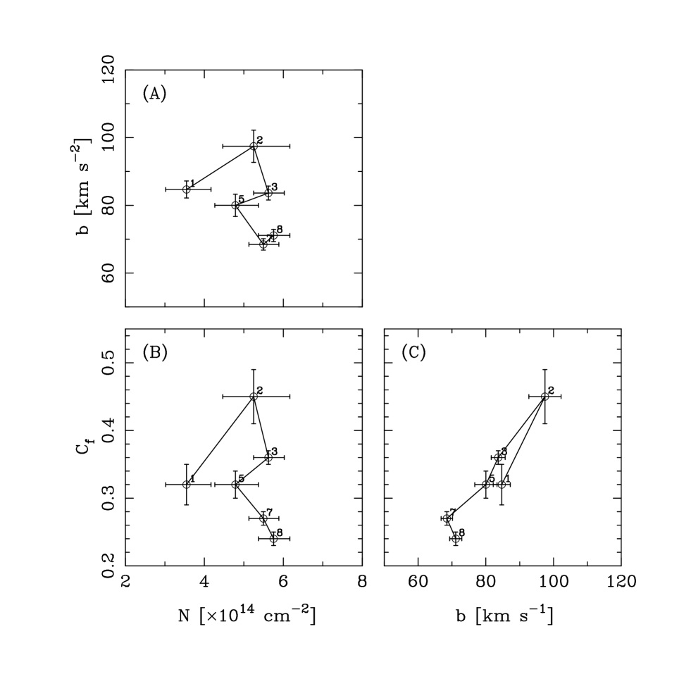
Figure 6: The relationship between (a) column density and Doppler parameter, (b) column density and coverage fraction, and (c) Doppler parameter and coverage fraction, with 1$\sigma$ error bars for the narrow component of the C IV mini-BAL in System A. Each point is labeled with the epoch number.

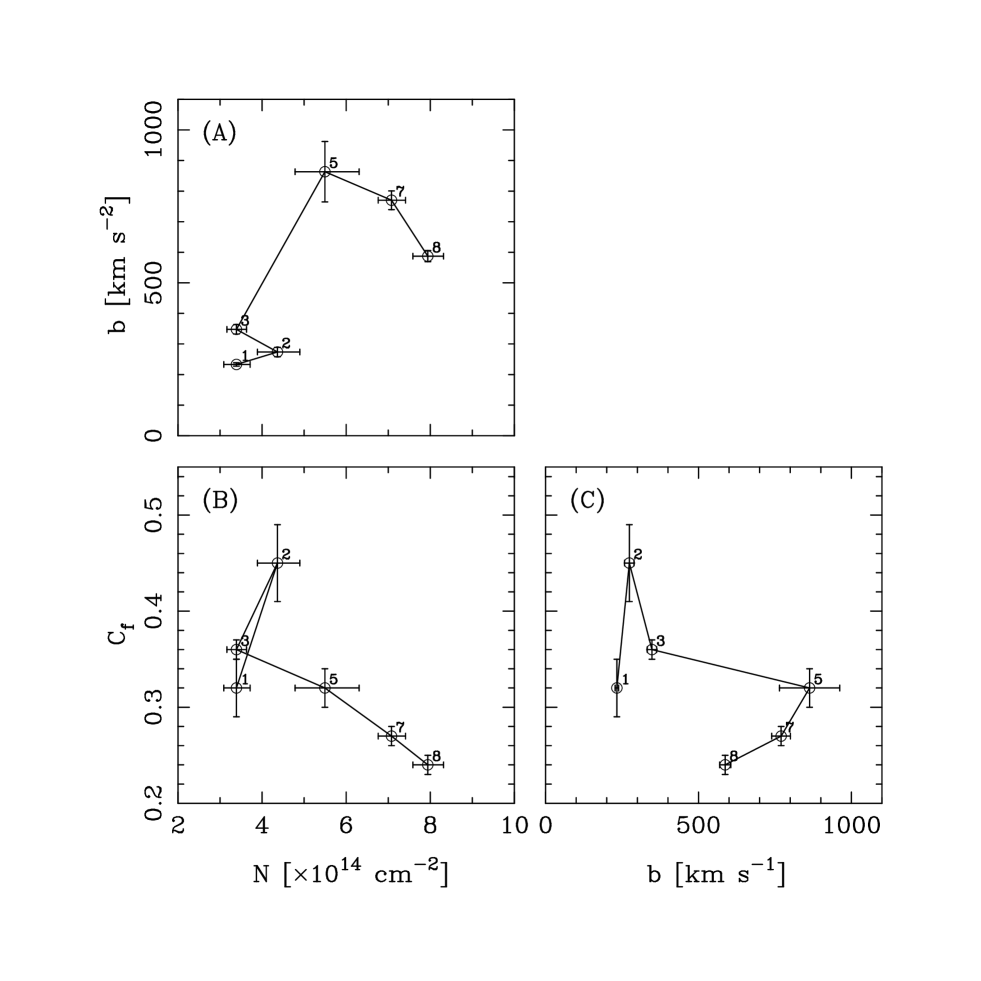
Figure 7: Same as Figure 6, but for the broad component of the C IV mini-BAL in System A. The error bars here are comparable to those of the narrow component shown in Figure 6, although the line center in the broad component is highly uncertain. This is because the fit parameters plotted here are not strongly affected by the error of the line center; the column density and coverage fraction are mainly determined by the depth around the line center, and the Doppler parameter is set primarily by the line width.

We have looked for correlated changes in all of the above parameters of the mini-BAL profile by plotting them against each other. In Figures 6 and 7, respectively, we show the relevant plots for the narrow and broad components of the mini-BAL. Other than a tentative trend between $C_{f}$ and $b$ in Figure 6 and between $C_{f}$ and $N_{\rm C\;IV}$ in Figure 7, we see no convincing correlation. This lack of correlated variability between model parameters is an important clue, which we take into consideration in our later discussion.

The observed shift velocity represents the ejection velocity of the absorber from the central engine projected along the line of sight. While the line center of the narrow component remains nearly constant, the broad component shifts by about 300 km s^-1 (${{v_{shift}}}\sim 10,100~{}{{{\rm km~{}s}^{-1}}}\rightarrow 10,400~{}{{{\rm km~{}s}^{-1}}}$) from epoch 1 to epoch 7. If this velocity shift is really due to the radiative pressure from the continuum source, the acceleration of the gas can be calculated to be $\sim$ 0.01 m s^-2. However, the measurement of the center of the broad component is highly uncertain, because the observed velocity shift is much smaller than the total line width because of self-blending of the blue and red members of the C IV doublet. Moreover, the center of the broad component moved in both directions (i.e., blueward and redward) during our observations. Although it is still not clear if there is a truly systematic increase in this parameter, we could regard the above value as an upper limit on the acceleration of the absorber.

4.2 NAL Systems

In addition to the mini-BAL system, we detected 8 NAL systems in the HS 1603+3820 spectra. For these NALs, we do not detect significant variability. Model fit results to the combined spectrum of the 6 Subaru observations (with a total exposure time of 8.9 hours and a S/N per 0.03 Å pixel of about 91 at $\lambda\sim 5370$ Å) are consistent with the results based on only the epoch 2 spectrum (a 1.7 hour exposure with $S/N\sim 49$ per pixel; Misawa et al. 2005), with only a few small exceptions as described below. In this section we discuss individual systems, other than system A (the mini-BAL). The profiles of the lines of these systems are shown on a common velocity scale in Figure 4(a–i).

System B

— We fit this strong C IV NAL, shown in Figure 4a,b, with 15 components, although Misawa et al. (2005) used 19 components. The coverage fractions of two components, 11 and 14, deviate from unity by more than 1$\sigma$, but both are heavily blended with other components and their $C_{f}$ values are not very reliable. All components in the N V NAL are consistent with full coverage. Only the epoch 8 spectrum covered the Si IV doublet of this system. For the Si IV doublet, only component 7 suggests partial coverage, but the model fit is not good around the left wing of this component. We conclude that this system does not show strong evidence for partial coverage, and is probably an intervening system, most likely a galaxy because of the strength of the low-ionization absorption lines.

System C

— The C IV NAL in this system with a simple absorption profile (see Figure 4c) is fitted with only one component, as in Misawa et al. (2005). Both fits are consistent with full coverage. We also did not find any evidence for time variability. Except for its small shift velocity, $\sim 430~{}{{{\rm km~{}s}^{-1}}}$, there is no evidence to suggest that this system is intrinsic.

System D

— Misawa et al. (2005) fitted this system’s C IV and Si IV profiles with 4 and 2 components, respectively, and did not find any partial coverage. However, we found an additional C IV component at ${{v_{shift}}}=-160~{}{{{\rm km~{}s}^{-1}}}$ from the system center that shows partial coverage, and we have no reason to suspect systematic error. The line profiles are shown in Figure 4d. This component was not studied by Misawa et al. (2005) because of a data defect. We also now find that component 1 in the Si IV NAL possibly shows partial coverage, although it was consistent with full coverage in the shorter exposure presented by Misawa et al. (2005). We also note that it is surprising that the C IV $\lambda$1548 is black at the position of this Si IV component if the partial coverage is true. However, the fact that partial coverage is apparent for both a Si IV and a C IV component suggests that this system may be an intrinsic system. The fact that this system is redshifted from the quasar systemic redshift also supports this idea. Although this system is located near the top of the C IV emission line, there is no residual flux at the position of the C IV doublet for components 4 and 5. These components must therefore cover both the continuum source and broad emission line region. We do not see any variability over the course of our observations.

System E

— Misawa et al. (2005) fitted the C IV NAL with only two components, and one of them showed evidence of partial coverage. However, our higher-S/N spectrum (shown in Figure 4e) requires 5 components to fit the C IV NAL, and three of them are consistent with full coverage. Although components 3 and 5 deviate from full coverage, they are heavily blended with the other components, so this result is quite uncertain. The shift velocity of the system is also extremely large, $\sim$60,000 km s^-1. There is no compelling reason to believe that this system is intrinsic to the quasar.

System F

— Our best-fitting model is almost consistent with the previous one, having the same number of components at almost the same positions (see Figure 4f). All components are consistent with full coverage except for component 1 that is blended with the strong component 2. This system also has a very large shift velocity, $\sim 50,000~{}{{{\rm km~{}s}^{-1}}}$. We consider it probable that this is an intervening system.

System G

— Because the C IV NAL in this system was positioned at the edge of the blue CCD of the HDS (around which bad pixels are common) in some of our observing setups, the absorption profiles are slightly or severely different in some spectra. Therefore, we combined only spectra from epochs 3, 7, and 8 (these are not affected by the data defect) to produce a final spectrum for this system (Figure 4g). We fit the C IV NAL with 6 components, and all of them are consistent with full coverage. Component 5 was not fitted by Misawa et al. (2005) because of the unphysical line ratio of the blue and red component, due to line blending. This system is probably an intervening system.

System H

— Two components are necessary to fit this C IV NAL (see Figure 4h). The shallower absorption feature, centered on component 2, has an unphysical ratio of its blue and red members. Probably the blue member is contaminated by other lines. Only component 1 is useful, and it yields ${{C_{f}}}=1$. In this system, we again do not see any evidence of intrinsic properties.

System I

— This system was detected only in the epoch 8 spectrum, because it was not covered in the other epochs. We used 7 components to fit the C IV NAL (see Figure 4i). Component 4 may show partial coverage, but its $C_{f}$ value differs from unity by only slightly more than 1$\sigma$. The case for partial coverage for component 6 is somewhat more compelling, since the minfit fitting procedure yielded a value ${{C_{f}}}\ =0.87\pm 0.02$. Component 4 is not blended with other components, and component 6 is only weakly blended. Although the S/N for this spectrum is not very high in the relevant region, this system may be another candidate for an intrinsic system.

5 DISCUSSION: THE ORIGIN OF TIME VARIABILITY

In view of the observational constraints derived above, we evaluate here different scenarios for the origin of the variability of the C IV mini-BAL. A fundamental assumption underlying our discussion is that the kinematic components making up system A represent parcels of absorbing gas at different positions along the line of sight. In effect, we assume that the absorber is embedded in an accelerating outflow from the quasar, thus the blueshift of a kinematic component increases with its distance from the quasar continuum source.

A very important observational clue from the data presented above is the fact that all the kinematic components of the mini-BAL system vary in concert (i.e., the depths of all troughs increase or decrease together). These changes appear to be driven largely by changes in the coverage fraction, as shown in Figure 5. Other physical parameters ($N_{\rm C\;IV}$ and $b$) are varying as well, but there does not seem to be an obvious correlation between changes of different profile parameters, at least in the bluest troughs of the mini-BAL (see Figures 6 and 7).

5.1 Transverse Motion of a Homogeneous Absorber

In Misawa et al. (2005) we favored an interpretation in which motion of the (homogeneous) absorber across the line (or cylinder) of sight causes the observed variability (see also Hamann et al. 1997a). The assumed scenario is depicted in the cartoon of Figure 2a of Hamann & Sabra (2004). With time, an increasing fraction of the cylinder of sight was covered by the absorber, leading to changes in the coverage fraction. In this context and based on two snapshots of the spectrum, we derived a transverse velocity of 8,000 km s^-1 and a constraint of $r<0.2$ pc on the distance of the absorber from the continuum source (see details in Misawa et al. 2005).

That model was motivated largely by the observation that the coverage fraction was the only quantity that changed substantially between the first two observations. The subsequent observations show that scenario to be too simple, namely the column density of the absorber changes with time as well, suggesting that the absorber is inhomogeneous and its internal structure plays an important role in the variability of the mini-BAL profile. Thus, a more plausible scenario is the one depicted in Figure 2b of Hamann & Sabra (2004) and in Figure 5 of de Kool, Korista, & Arav (2002), where the absorbing medium is inhomogeneous, with clumps spanning a range of column densities scattered over the cylinder of sight.

There is a remaining difficulty with this scenario, however. The fact that all the troughs in the mini-BAL vary in concert would require a coincidence between the motions of the individual clumps. More specifically, the projected areas of all the clumps within the cylinder of sight should vary in the same way (i.e., rise and fall with time in the same manner for all clumps). We consider such a coordinated sequence of variations rather unlikely, therefore, we regard this interpretation as implausible. We note that if future observations show this pattern to be common, then this interpretation can be conclusively rejected.

5.2 Internal Motions in the Absorbing Gas

At first glance, compression of the absorber might be able to produce a trend similar to that of Figure 7b, where the coverage fraction decreases as the column density increases in one of the kinematic components of the mini-BAL. However, on closer examination, such a compression would require highly supersonic motions within the absorber. Assuming the background continuum source size is 0.02 pc (this is the UV-emitting region of the accretion disk; see Misawa et al. 2005), a change in the coverage fraction from 0.36 to 0.27 within 0.13 years (epochs 5 and 7) implies a speed of order $10^{4}~{}{{{\rm km~{}s}^{-1}}}$. In comparison, the speed of sound in a $\sim 10^{4}$ K gas is only $10~{}{{{\rm km~{}s}^{-1}}}$. Thus we consider such a scenario untenable.

5.3 Scattering of Continuum Photons Around the Absorber

The observed partial coverage signature can, in principle, be explained if continuum photons are re-directed by a scattering medium towards the observer, when they were initially traveling in a different direction. Thus, the absorber can be homogeneous and its projected size need not be smaller than the cylinder of sight towards the continuum source. The dilution of the troughs by photons scattered around the absorber can change with time as the absorber moves relative to the scattering medium or as the conditions in the scattering medium change. In the context of this scenario, the apparent coverage fraction can vary according to the behavior of the scattering medium. Moreover, the variations of the coverage fraction need not be tied in any way to variations of other parameters of the absorber, such as the C IV column density, the $b$-parameter, or the shift velocity. This idea can be tested observationally through spectropolarimetry. In particular, we would expect the fractional polarization in the absorption mini-BAL troughs to be higher than in the continuum (see the analogous test in BAL quasars by Brotherton et al. 1997, Ogle et al. 1999, and Lamy & Hutsemékers 2000, for example). Furthermore, we would also expect this fractional polarization to increase as the coverage fraction decreases.

5.4 Change of Ionization State of the Absorbing Gas

Changes in the level of the ionizing continuum can also bring about absorption-line variability since they change the relative ionic populations in the absorber (in this particular case, the relative populations of C III, C IV and C V). In principle, a monotonic change in the continuum intensity can produce a non-monotonic change in the absorption line strength. For example, an absorber initially at a low ionization state that sees a rising ionizing flux will first respond with an increase in the strength of its C IV absorption lines (as C III$\;\rightarrow\;$C IV) and then with a decrease (as C IV$\;\rightarrow\;$C V). The variability time scale of the absorption lines provides an upper limit on the ionization or recombination time of the absorbing gas, hence its electron density (see the detailed discussion in Hamann et al. 1997b and Narayanan et al. 2004). The density limit can be obtained from $n_{e}\geq(\alpha_{r}t_{var})^{-1}$, where $\alpha_{r}$ is a recombination coefficient and $t_{var}$ is a variability time scale. This is a simplified picture in which the gas is in ionization equilibrium and C IV is the dominant ionic species of C.

Since the C IV ionic column densities have fluctuated up and down more than once over the course of our monitoring observations, the ionizing continuum seen by the absorber must be fluctuating too. Moreover, the continuum intensity must be fluctuating by at least a factor of 3 on rest-frame time scales of 6 months or less to produce the observed changes in the C IV ionic column density (see the calculations of Hamann 1997). Taking this interpretation at face value (but see discussion below), we can use the shortest variability time scale that we have observed (16 days in the quasar rest frame, epochs 5$\;\rightarrow\;$7; see Fig. 5) to constrain the density of the gas. We consider both an increase and a decrease in the ionization state of the gas as a cause for the observed change in the C IV column density (i.e., C III$\;\rightarrow\;$C IV or C V$\;\rightarrow\;$C IV), with respective recombination coefficients of $5.3\times 10^{-12}~{}{\rm cm^{3}~{}s^{-1}}$ and $2.8\times 10^{-12}~{}{\rm cm^{3}~{}s^{-1}}$ (from Arnaud & Rothenflugh 1986; assuming a nominal gas temperature of 20,000 K, following Hamann 1997). Thus we obtain a limit on the electron density of $n_{e}>1\times 10^{5}~{}{{{\rm cm}^{-3}}}$, using the methodology of Narayanan et al. (2004) and a bolometric luminosity of $L_{bol}=2.5\times 10^{48}~{}{\rm erg~{}s}^{-1}$ (Misawa et al. 2005). To convert this limit to a limit on the distance of the absorber from the continuum source, $r$, we must assume a value of the ionization parameter. If the C IV column density fluctuations reflect conversions of C III$\;\leftrightarrow\;$C IV in a lower-ionization absorber, then the calculations of Hamann (1997) indicate an ionization parameter of $U\sim 0.002$ and lead to $r<8$ kpc. If, on the other hand, the C IV column density fluctuations reflect conversions of C V$\;\leftrightarrow\;$C IV in a higher-ionization absorber, then the calculations of Hamann (1997) indicate an ionization parameter of $U\sim 0.06$ and lead to $r<1$ kpc. In this context the simultaneous variability of all the mini-BAL troughs implies that these troughs should represent gas parcels of similar densities for the following reason. Since all absorbing gas parcels must be within the cylinder of sight to the continuum source, the time lag between changes in the continuum intensity at the source and our observation of a change in the mini-BAL profile is the sum of the light travel times from the continuum source to the absorber and from the absorber to the observer, plus the recombination time of the gas. The sum of light travel times is the same regardless of the location of a gas parcel along the cylinder of sight, therefore, a difference in time lag can only result from different recombination times, i.e., different gas densities. We can then conclude that the density does not vary significantly across the line profile, which implies in turn that the shape of the mini-BAL profile is determined primarily by the combination of column density (i.e., physical thickness) and coverage fraction as a function of velocity.

Fluctuations in the ionization state of the absorber are an attractive explanation of the observed variations in the strength of the mini-BAL in HS 1603+3820. However, the mini-BAL appears to vary much faster than any expected variations in the UV continuum of such a luminous quasar (see for example, Giveon et al. 1999, Hawkins 2001, and Kaspi et al. 2007). Moreover, Fleming & Kennefick (2006) found no variability of this particular quasar in 10 days in the observed frame. Therefore we propose that the variations of the ionizing continuum seen by the absorber are caused by a screen of variable optical depth between it and the (relatively steady) continuum source. This screen could be the ionized, clumpy, inner part of the outflow, i.e., the shielding or hitchhiking gas invoked in the outflow models of Murray et al. (1995), and arising naturally in the more detailed calculations of Proga et al. (2000). The two-dimensional, axisymmetric models of Proga et al. (2000) also show that disk winds can be accelerated up to 15,000 km s^-1, and that they are unsteady and generate dense knots periodically. The time variability seen in the mini-BAL system of HS 1603+3820 may be related to this mechanism. The conditions in the screen may be similar to those of “warm” absorbers, observed in the X-ray spectra of many Seyfert galaxies, where it often co-exists with a UV absorber (e.g., Crenshaw et al. 1999). We note, by way of example, that models for the warm absorbers in NGC 5548, IRAS 1339+2438, and NGC 3783 require multiple ionization phases for an adequate fit to the X-ray spectrum (Kaastra et al. 2000, Sako et al. 2001, Blustin et al. 2002), one of which may fulfill the requirements for the inner screen.

If the optical depth of the screen at wavelengths around the C IV edge is close to unity, then small fluctuations in the column density can cause large changes in the shape and intensity of the transmitted ionizing continuum (e.g., Fig. 6 of Murray et al. 1995, or Fig. 1 of Hamann 1995), leading to the observed changes in the mini-BAL of HS 1603+3820. This may be analogous to the best-studied warm absorber, in the Seyfert galaxy NGC 3783, where fluctuations in the ionization structure of the absorbing gas have been observed over the course of 6 months (e.g., Netzer et al. 2003). There is also evidence that the opacity of the warm absorber in NGC 3783 fluctuates over time intervals as short as a month, in response to variations in the X-ray continuum by a factor of 2 (Krongold et al. 2005). Within this context we can also understand why the variations in the coverage fraction of the mini-BAL gas are unrelated to variations of its column density. Because both media can be clumpy and since differential rotation of the wind causes the inner screen to move faster than the mini-BAL gas across the cylinder of sight, the intensity of the continuum transmitted through the screen and received by the mini-BAL gas would vary with time. Moreover, the coverage fraction need not be correlated with the intensity of the transmitted continuum.

We have considered the possibility that one of the observed NAL systems at smaller blueshifts relative to the quasar could represent the inner screen. However, none of the three candidate C IV systems, B, C, and D, can satisfy the requirements for the screen. The very fact that they have C IV absorption lines suggests that their ionization state is too low, and moreover, systems B and D have even lower-ionization lines. In addition, none of the three systems are variable, which is necessary in order for the screen to perform the desired function. More promising ways of finding the screen signature are X-ray observations in search of the classic warm absorber feature, O VII and O VIII edges. Thus, we will be able to determine which of the Ly$\alpha$ absorption lines seen at shorter wavelengths might be associated with the screen material.

6 SUMMARY AND CONCLUSIONS

We have been monitoring the absorption lines in the spectrum of the quasar HS 1603+3820 since 2002, using the Subaru and Hobby-Eberly Telescopes. We have obtained six Subaru+HDS and two HET+MRS spectra spanning an interval of approximately 1.2 years in the quasar rest frame and probing rest-frame time scales as short as 16 days. We have determined the physical parameters of the 9 absorption-line systems by fitting Voigt models to the line profiles. Our main results are as follows:

1. We detect one C IV mini-BAL and eight C IV NAL systems in the quasar spectrum. The partial coverage signature and time variability of the mini-BAL show it to be intrinsic to the quasar. Two of the NAL systems (D and I) may also be intrinsic, based upon our partial coverage analysis.

2. We are able to fit models only to the bluest portion of the C IV mini-BAL profile where self-blending is not severe. All fit parameters (i.e., column density, Doppler parameter, coverage fraction, and shift velocity) as well as the total equivalent width of the system vary significantly with time, even on short time scales. However, the profile parameters do not appear to change in concert with each other, with one exception: the equivalent widths of all the troughs in this system vary together and approximately follow the variations of the coverage fraction determined from the model fits.

3. We have examined a number of ways of explaining the above variations of the C IV mini-BAL and we have found two viable possibilities. The first possibility is that the observed partial coverage signature is the result of continuum photons scattering around the absorber and into our cylinder of sight. The observed changes in mini-BAL equivalent widths are thus produced by variations in the scattered continuum that dilutes the absorption troughs. In the second possibility, the illumination of the UV absorber fluctuates on short time scales by a factor of up to 3. We suggest that these fluctuations are caused by a screen of variable optical depth between the mini-BAL gas and the continuum source. This screen might be identified with the shielding gas invoked or predicted in some outflow models. Moreover, it could be analogous to the “warm” absorbers observed in the X-ray spectra of Seyfert galaxies and some quasars. This picture can also explain the variations in the coverage fraction, which appear to be unrelated to the ionic column density changes.

Table 1: Log of Monitoring Observations

		Time		Wavelength Coverage	Exposure	Resolving
Epoch	Date	(years)	Instrument	(Å)	(s)	Power	$S/N$
(1)	(2)	(3)	(4)	(5)	(6)	(7)	(8)
1	2002 Mar 23	0.00	Subaru+HDS	5080–6420	2700	45,000	46.5
2	2003 Jul 7	0.36	Subaru+HDS	3520–4850, 4930–6260	6000	45,000	48.7
3	2005 Feb 26	0.83	Subaru+HDS	3520–4855, 4925–6275	7100	36,000	43.0
4	2005 May 10	0.89	HET+MRS	4500–6200	1800	9,200	17.4
5	2005 Jun 29	0.92	Subaru+HDS	3530–4855, 4925–6280	3600	45,000	31.1
6	2005 Aug 3,8	0.95	HET+MRS	4500–6170	4000	9,200	28.5
7	2005 Aug 19	0.96	Subaru+HDS	3520–4850, 4920–6235	3600	36,000	43.6
8	2006 May 31–Jun 1	1.18	Subaru+HDS	4320–5630, 5740–7050	9000	45,000	52.5

Table 2: Best fit parameters of C IV mini-BAL

			narrow component						broad component
		Time	$v_{shift}$	log$N$	$b$	$C_{f}$	$EW^{b}$		$v_{shift}$	log$N$	$b$	$C_{f}$	$EW^{b}$
Epoch	Date	(yrs)	(km s-1)	(cm-2)	(km s-1)		(Å)		(km s-1)	(cm-2)	(km s-1)		(Å)
(1)	(2)	(3)	(4)	(5)	(6)	(7)	(8)		(9)	(10)	(11)	(12)	(13)
1	2002 Mar 23	0.00	10648	14.55$\pm$0.07	85$\pm$3	0.32$\pm$0.03	1.49		10118	14.53$\pm$0.04	233$\pm$ 6	0.32$\pm$0.03	1.88
2	2003 Jul 7	0.36	10637	14.72$\pm$0.07	98$\pm$5	0.45$\pm$0.04	2.79		10273	14.64$\pm$0.05	274$\pm$15	0.45$\pm$0.04	3.32
3	2005 Feb 26	0.83	10644	14.75$\pm$0.03	84$\pm$2	0.36$\pm$0.01	2.15		10309	14.53$\pm$0.03	348$\pm$15	0.36$\pm$0.01	2.22
4	2005 May 10 c	0.89	10643	14.70	81	0.33	1.83		10259	14.67	692	0.33	2.86
5	2005 Jun 29	0.92	10642	14.68$\pm$0.05	80$\pm$3	0.32$\pm$0.02	1.72		10235	14.74$\pm$0.06	863$\pm$99	0.32$\pm$0.02	3.20
6	2005 Aug 3–8 d	0.95	10641	14.72	71	0.28	1.49		10345	14.82	793	0.28	3.29
7	2005 Aug 19	0.96	10641	14.74$\pm$0.03	69$\pm$2	0.27$\pm$0.01	1.43		10381	14.85$\pm$0.02	770$\pm$31	0.27$\pm$0.01	3.36
8	2006 May 31–Jun 1	1.18	10637	14.76$\pm$0.03	71$\pm$2	0.24$\pm$0.01	1.32		10291	14.90$\pm$0.02	587$\pm$18	0.24$\pm$0.01	3.27

Table 3: Metal lines in the combined spectrum

Line ID	$\lambda_{obs}$	$z_{abs}$	$v_{shift}$	$\log\;N$	$b$	$C_{f}$
	(Å)		(km s-1)	(cm-2)	(km s-1)
(1)	(2)	(3)	(4)	(5)	(6)	(7)
System B : $z_{abs}=2.4785$
C IV $\lambda$1548 / C IV $\lambda$1551 ($W_{obs}$ = 4.58 / 3.32 Å)
1…………	5381.8	2.47618	5627	13.36 $\pm$ 0.01	8.2 $\pm$ 0.2	1.00
2…………	5382.2	2.47642	5606	14.16 $\pm$ 0.03	6.3 $\pm$ 0.2	1.00
3…………	5382.8	2.47685	5569	13.52 $\pm$ 0.01	22.4 $\pm$ 0.4	1.00
4…………	5383.8	2.47749	5514	13.83 $\pm$ 0.00	15.6 $\pm$ 0.1	1.00
5…………	5383.9	2.47752	5511	14.69 $\pm$ 0.46	5.5 $\pm$ 1.1	1.00${}^{+0.03}_{-0.03}$
6…………	5384.3	2.47779	5488	12.87 $\pm$ 0.29	4.1 $\pm$ 2.1	0.90${}^{+0.60}_{-0.40}$
7…………	5384.5	2.47793	5476	13.58 $\pm$ 0.01	6.7 $\pm$ 0.2	1.00
8…………	5385.0	2.47826	5447	14.06 $\pm$ 0.00	14.8 $\pm$ 0.2	1.00
9…………	5385.6	2.47862	5416	13.96 $\pm$ 0.10	14.7 $\pm$ 2.2	0.97${}^{+0.03}_{-0.03}$
10………..	5386.2	2.47899	5384	14.13 $\pm$ 0.00	27.1 $\pm$ 0.2	1.00
11………..	5386.2	2.47899	5384	13.62 $\pm$ 0.21	5.6 $\pm$ 1.2	0.76${}^{+0.18}_{-0.18}$
12………..	5387.1	2.47959	5333	12.96 $\pm$ 0.21	7.3 $\pm$ 1.0	1.00${}^{+0.66}_{-0.43}$
13………..	5387.4	2.47977	5317	13.74 $\pm$ 0.01	7.8 $\pm$ 0.1	1.00
14………..	5388.2	2.48028	5273	13.56 $\pm$ 0.18	28.1 $\pm$ 2.2	0.45${}^{+0.49}_{-0.17}$
15………..	5388.6	2.48055	5250	14.03 $\pm$ 0.03	4.7 $\pm$ 0.1	1.00
N V $\lambda$1239 / N V $\lambda$1243 ($W_{obs}$ = 0.35 / 0.19 Å)
1…………	4308.0	2.47748	5514	13.26 $\pm$ 0.01	7.7 $\pm$ 0.3	1.00
2…………	4308.4	2.47784	5483	12.73 $\pm$ 0.06	9.4 $\pm$ 1.5	1.00
3…………	4308.9	2.47824	5449	13.13 $\pm$ 0.06	19.7 $\pm$ 2.7	1.00
4…………	4309.6	2.47882	5399	13.22 $\pm$ 0.05	28.2 $\pm$ 4.0	1.00
Si IV $\lambda$1394 / Si IV $\lambda$1403 ($W_{obs}$ = 1.59 / 1.05 Å)
1…………	4845.2	2.47635	5612	12.44 $\pm$ 0.03	15.5 $\pm$ 0.8	1.00
2…………	4845.3	2.47642	5606	13.20 $\pm$ 0.01	4.0 $\pm$ 0.1	1.00
3…………	4846.8	2.47751	5512	12.49 $\pm$ 0.01	7.5 $\pm$ 0.2	1.00
4…………	4847.4	2.47793	5476	12.72 $\pm$ 0.01	2.9 $\pm$ 0.1	1.00
5…………	4847.8	2.47824	5449	13.05 $\pm$ 0.10	21.3 $\pm$ 0.9	0.94${}^{+0.29}_{-0.21}$
6…………	4848.3	2.47860	5418	13.12 $\pm$ 0.00	9.3 $\pm$ 0.1	1.00
7…………	4848.9	2.47899	5384	13.05 $\pm$ 0.07	11.9 $\pm$ 0.3	0.69${}^{+0.08}_{-0.07}$
8…………	4849.7	2.47960	5332	12.98 $\pm$ 0.01	27.7 $\pm$ 0.4	1.00
9…………	4849.9	2.47976	5318	12.86 $\pm$ 0.01	4.6 $\pm$ 0.1	1.00
10………..	4851.0	2.48054	5251	13.39 $\pm$ 0.01	4.9 $\pm$ 0.1	1.00
Si IIi $\lambda$1207 ($W_{obs}$ = 4.68 Å)
1…………	4194.8	2.47687	5567	15.14 $\pm$ 0.30	20.1 $\pm$ 1.4	1.00
2…………	4195.8	2.47770	5496	13.97 $\pm$ 0.01	84.7 $\pm$ 1.6	1.00
3…………	4196.9	2.47857	5420	14.31 $\pm$ 2.23	6.9 $\pm$ 4.5	1.00
4…………	4197.4	2.47903	5381	12.57 $\pm$ 0.04	8.4 $\pm$ 0.8	1.00
5…………	4198.0	2.47949	5341	13.71 $\pm$ 1.57	4.6 $\pm$ 2.7	1.00
6…………	4198.3	2.47976	5318	14.43 $\pm$ 0.57	3.1 $\pm$ 0.7	1.00
7…………	4198.3	2.47971	5322	13.06 $\pm$ 0.03	32.7 $\pm$ 1.4	1.00
8…………	4199.2	2.48052	5252	13.99 $\pm$ 0.38	5.6 $\pm$ 0.7	1.00
9…………	4200.1	2.48122	5192	13.10 $\pm$ 2.41	2.2 $\pm$ 3.2	1.00
10………..	4200.3	2.48136	5180	12.51 $\pm$ 0.04	4.8 $\pm$ 0.7	1.00
C II $\lambda$1335($W_{obs}$ = 2.07 Å)
1…………	4639.4	2.47642	5606	13.52 $\pm$ 0.07	2.6 $\pm$ 0.3	1.00
2…………	4641.7	2.47811	5460	14.06 $\pm$ 0.01	11.9 $\pm$ 0.2	1.00
3…………	4642.2	2.47852	5425	14.41 $\pm$ 0.03	13.9 $\pm$ 0.4	1.00
4…………	4642.5	2.47871	5408	14.15 $\pm$ 2.21	2.6 $\pm$ 3.4	1.00
5…………	4642.9	2.47904	5380	12.98 $\pm$ 0.02	9.9 $\pm$ 0.9	1.00
6…………	4643.4	2.47944	5345	13.08 $\pm$ 0.02	7.0 $\pm$ 0.6	1.00
7…………	4643.8	2.47970	5323	13.97 $\pm$ 0.08	4.3 $\pm$ 0.9	1.00
8…………	4643.9	2.47981	5314	12.72 $\pm$ 1.02	10.6 $\pm$13.0	1.00
9…………	4644.7	2.48037	5265	12.26 $\pm$ 0.70	1.1 $\pm$ 5.1	1.00
10………..	4644.9	2.48052	5252	14.92 $\pm$ 0.80	3.6 $\pm$ 0.9	1.00
11………..	4645.8	2.48120	5194	15.33 $\pm$ 1.70	2.7 $\pm$ 1.2	1.00
12………..	4646.0	2.48134	5182	13.89 $\pm$ 0.08	3.7 $\pm$ 0.6	1.00
13………..	4646.3	2.48162	5158	12.72 $\pm$ 0.03	5.0 $\pm$ 0.8	1.00
Al II $\lambda$1671 ($W_{obs}$ = 0.90 Å)
1…………	5811.2	2.47814	5458	11.95 $\pm$ 0.01	10.6 $\pm$ 0.4	1.00
2…………	5811.9	2.47856	5421	12.92 $\pm$ 0.02	8.8 $\pm$ 0.1	1.00
3…………	5813.4	2.47944	5345	11.28 $\pm$ 0.03	4.2 $\pm$ 0.9	1.00
4…………	5813.9	2.47972	5321	11.70 $\pm$ 0.01	4.0 $\pm$ 0.4	1.00
5…………	5815.2	2.48053	5252	12.57 $\pm$ 3.50	1.5 $\pm$ 3.2	1.00
6…………	5816.4	2.48121	5193	11.84 $\pm$ 0.18	1.7 $\pm$ 1.1	1.00
7…………	5816.6	2.48135	5181	11.50 $\pm$ 0.04	3.5 $\pm$ 1.2	1.00
Si II $\lambda$1260 ($W_{obs}$ = 1.85 Å)
1…………	4381.3	2.47607	5636	12.08 $\pm$ 0.02	4.1 $\pm$ 0.6	1.00
2…………	4381.7	2.47641	5607	13.26 $\pm$ 1.78	1.8 $\pm$ 1.5	1.00
3…………	4383.6	2.47791	5477	12.55 $\pm$ 2.19	1.5 $\pm$ 3.3	1.00
4…………	4383.9	2.47813	5458	13.11 $\pm$ 0.01	9.0 $\pm$ 0.4	1.00
5…………	4384.3	2.47845	5431	15.74 $\pm$ 0.39	1.9 $\pm$ 0.1	1.00
6…………	4384.6	2.47865	5414	13.48 $\pm$ 0.37	5.8 $\pm$ 1.9	1.00
7…………	4384.8	2.47887	5395	12.07 $\pm$ 0.04	3.2 $\pm$ 1.5	1.00
8…………	4385.1	2.47905	5379	11.97 $\pm$ 0.03	3.7 $\pm$ 0.9	1.00
9…………	4385.6	2.47944	5345	12.22 $\pm$ 0.02	5.9 $\pm$ 0.5	1.00
10………..	4385.9	2.47971	5322	13.03 $\pm$ 0.07	4.1 $\pm$ 0.3	1.00
11………..	4386.9	2.48052	5252	14.13 $\pm$ 0.28	3.1 $\pm$ 0.3	1.00
12………..	4387.8	2.48122	5192	13.63 $\pm$ 1.30	3.2 $\pm$ 2.0	1.00
13………..	4388.0	2.48135	5181	12.93 $\pm$ 4.77	2.0 $\pm$ 6.3	1.00
Fe II $\lambda$1608 ($W_{obs}$ = 0.13 Å)
1…………	5595.1	2.47857	5420	13.65 $\pm$ 0.01	4.6 $\pm$ 0.1	1.00
O I $\lambda$1302 ($W_{obs}$ = 0.29 Å)
1…………	4529.7	2.47855	5422	14.58 $\pm$ 0.03	6.9 $\pm$ 0.2	1.00
2…………	4533.2	2.48125	5190	13.41 $\pm$ 0.02	10.7 $\pm$ 0.8	1.00
Si II $\lambda$1527 ($W_{obs}$ = 2.68 Å)a
1…………	5303.3	2.47369	5841	13.05	21.0	1.00
2…………	5304.0	2.47416	5801	13.12	22.8	1.00
3…………	5304.9	2.47476	5749	12.95	21.4	1.00
4…………	5306.4	2.47570	5668	13.62	11.1	1.00
5…………	5307.6	2.47647	5602	13.04	13.1	1.00
6…………	5310.1	2.47815	5457	13.24	14.2	1.00
7…………	5310.8	2.47857	5420	14.07	11.2	1.00
8…………	5312.6	2.47976	5318	13.17	12.3	1.00
9…………	5313.8	2.48055	5250	13.43	5.2	1.00
10………..	5314.8	2.48124	5190	13.22	7.5	1.00
11………..	5315.2	2.48147	5171	13.46	11.6	1.00
System C : $z_{abs}=2.5370$
C IV $\lambda$1548 / C IV $\lambda$1551 ($W_{obs}$ = 0.24 / 0.14 Å)
1…………	5475.9	2.53693	430	13.41 $\pm$0.05	10.9 $\pm$ 0.2	0.94${}^{+0.08}_{-0.07}$
System D : $z_{abs}=2.5532$
C IV $\lambda$1548 / C IV $\lambda$1551 ($W_{obs}$ = 1.40 / 1.23 Å)
1…………	5498.0	2.55125	–782	13.18 $\pm$ 0.22	3.0 $\pm$ 0.7	0.30${}^{+0.14}_{-0.09}$
2…………	5500.1	2.55261	–897	13.05 $\pm$ 0.14	4.5 $\pm$ 0.6	0.81${}^{+0.24}_{-0.18}$
3…………	5500.4	2.55280	–913	13.54 $\pm$ 0.15	8.2 $\pm$ 3.3	0.23${}^{+0.05}_{-0.05}$
4…………	5501.0	2.55314	–942	14.26 $\pm$ 0.02	11.7 $\pm$ 0.5	0.99${}^{+0.02}_{-0.02}$
5…………	5501.5	2.55351	–973	16.66 $\pm$ 0.06	5.6 $\pm$ 0.1	0.99${}^{+0.02}_{-0.02}$
Si IV $\lambda$1394 / Si IV $\lambda$1403 ($W_{obs}$ = 0.49 / 0.34 Å)
1…………	4952.2	2.55313	–941	13.05 $\pm$ 0.06	9.4 $\pm$ 0.3	0.66${}^{+0.06}_{-0.06}$
2…………	4952.7	2.55350	–972	13.41 $\pm$ 0.02	8.4 $\pm$ 0.1	0.96${}^{+0.03}_{-0.03}$
System E : $z_{abs}=1.8875$
C IV $\lambda$1548 / C IV $\lambda$1551 ($W_{obs}$ = 0.67 / 0.41 Å)
1…………	4469.8	1.88708	60493	13.07 $\pm$ 0.30	7.5 $\pm$ 1.3	0.73${}^{+1.05}_{-0.43}$
2…………	4470.1	1.88730	60471	13.61 $\pm$ 0.08	14.2 $\pm$ 2.3	0.93${}^{+0.08}_{-0.08}$
3…………	4470.5	1.88753	60448	13.35 $\pm$ 0.16	8.4 $\pm$ 2.7	0.64${}^{+0.18}_{-0.16}$
4…………	4470.7	1.88771	60430	13.06 $\pm$ 0.33	7.7 $\pm$ 3.1	0.78${}^{+1.09}_{-0.45}$
5…………	4471.0	1.88788	60414	13.34 $\pm$ 0.17	10.8 $\pm$ 1.6	0.67${}^{+0.26}_{-0.19}$
System F : $z_{abs}=1.9644$
C IV $\lambda$1548 / C IV $\lambda$1551 ($W_{obs}$ = 1.41 / 1.08 Å)
1…………	4587.4	1.96305	52980	13.49 $\pm$ 0.12	11.2 $\pm$ 0.9	0.52${}^{+0.10}_{-0.09}$
2…………	4587.7	1.96327	52959	13.86 $\pm$ 0.02	5.9 $\pm$ 0.2	1.00
3…………	4588.0	1.96345	52941	13.78 $\pm$ 0.01	7.5 $\pm$ 0.3	1.00
4…………	4588.6	1.96381	52906	13.04 $\pm$ 0.44	5.1 $\pm$ 0.9	0.37${}^{+\infty}_{-0.28}$
5…………	4589.4	1.96436	52852	14.00 $\pm$ 0.03	8.3 $\pm$ 0.2	0.99${}^{+0.03}_{-0.03}$
6…………	4589.8	1.96459	52829	13.26 $\pm$ 0.17	9.4 $\pm$ 1.2	0.71${}^{+0.30}_{-0.22}$
7…………	4590.2	1.96486	52803	13.40 $\pm$ 0.08	8.3 $\pm$ 0.5	0.89${}^{+0.11}_{-0.10}$
8…………	4590.5	1.96506	52783	12.85 $\pm$ 0.02	5.9 $\pm$ 0.4	1.00
System G : $z_{abs}=2.0701$
C IV $\lambda$1548 / C IV $\lambda$1551 ($W_{obs}$ = 1.24 / 0.74 Å)
1…………	4752.1	2.06947	42665	12.70 $\pm$ 0.03	11.6 $\pm$ 1.1	1.00
2…………	4752.6	2.06974	42639	13.75 $\pm$ 0.00	10.0 $\pm$ 0.1	1.00
3…………	4752.9	2.06997	42617	14.04 $\pm$ 0.04	14.8 $\pm$ 1.4	1.00${}^{+0.02}_{-0.02}$
4…………	4753.2	2.07016	42599	13.47 $\pm$ 0.01	12.0 $\pm$ 0.2	1.00
5…………	4753.7	2.07045	42571	13.01 $\pm$ 0.02	9.1 $\pm$ 0.6	1.00
6…………	4754.0	2.07070	42547	12.56 $\pm$ 0.05	11.8 $\pm$ 1.8	1.00
Si IV $\lambda$1403 ($W_{obs}$ = 0.23 Å)
1…………	4306.3	2.06984	42629	13.16 $\pm$ 0.02	14.6 $\pm$ 0.7	1.00
2…………	4306.6	2.07010	42604	12.83 $\pm$ 0.03	7.3 $\pm$ 0.6	1.00
System H : $z_{abs}=2.2653$
C IV $\lambda$1548 / C IV $\lambda$1551 ($W_{obs}$ = 0.14 / 0.09 Å)
1…………	5055.2	2.26521	24357	13.05 $\pm$ 0.22	5.9 $\pm$ 0.5	0.75${}^{+0.40}_{-0.28}$
2…………	5055.5	2.26542	24337	13.85 $\pm$ 0.16	13.8 $\pm$ 2.8	0.14${}^{+0.03}_{-0.02}$
Si IIi $\lambda$1207 ($W_{obs}$ = 0.17 Å)
1…………	3939.5	2.26520	24357	12.76 $\pm$ 0.13	4.2 $\pm$ 0.8	1.00
2…………	3939.6	2.26534	24345	11.82 $\pm$ 0.21	1.7 $\pm$ 3.6	1.00
System I : $z_{abs}=2.1753$
C IV $\lambda$1548 / C IV $\lambda$1551 ($W_{obs}$ = 0.66 / 0.40 Å)
1…………	4914.9	2.17460	32722	12.83 $\pm$ 0.01	9.9 $\pm$ 0.5	1.00
2…………	4915.2	2.17481	32703	12.97 $\pm$ 0.22	8.7 $\pm$ 1.4	0.90${}^{+0.84}_{-0.43}$
3…………	4915.4	2.17494	32691	12.25 $\pm$ 0.03	2.0 $\pm$ 1.3	1.00
4…………	4915.8	2.17520	32666	13.33 $\pm$ 0.11	14.8 $\pm$ 0.7	0.70${}^{+0.24}_{-0.16}$
5…………	4916.2	2.17542	32646	13.17 $\pm$ 0.46	0.8 $\pm$ 0.6	0.37${}^{+1.04}_{-0.26}$
6…………	4916.4	2.17558	32631	13.65 $\pm$ 0.02	8.6 $\pm$ 0.3	0.87${}^{+0.02}_{-0.02}$
7…………	4916.7	2.17578	32612	12.76 $\pm$ 0.03	27.4 $\pm$ 2.4	1.00
Si IV $\lambda$ 1394 / Si IV $\lambda$1403 ($W_{obs}$ = 0.18 / 0.07 Å)
1…………	4424.6	2.17462	32720	11.96 $\pm$ 0.05	8.2 $\pm$ 1.7	1.00
2…………	4424.9	2.17480	32704	11.67 $\pm$ 0.08	1.2 $\pm$ 4.9	1.00
3…………	4425.1	2.17495	32690	11.74 $\pm$ 0.08	4.7 $\pm$ 2.1	1.00
4…………	4425.4	2.17519	32667	12.04 $\pm$ 0.04	9.3 $\pm$ 1.2	1.00
5…………	4426.0	2.17557	32632	12.51 $\pm$ 0.01	7.2 $\pm$ 0.3	1.00
Si IIi $\lambda$1207 ($W_{obs}$ = 0.27 Å)
1…………	3830.9	2.17524	32663	12.35 $\pm$ 0.03	7.7 $\pm$ 0.8	1.00
2…………	3831.4	2.17560	32629	12.61 $\pm$ 0.03	6.8 $\pm$ 0.5	1.00
Si II $\lambda$1527
1…………	(blending with Si IV $\lambda$1394 of System B)

Figure 1: Normalized spectrum of HS 1603+3820 after rebinning to 0.03 Å per pixel, and combining all 6 spectra taken with Subaru+HDS (see Table 1). C IV absorption systems and other metal lines are marked. Positions of the quasar emission lines of Ly$\alpha$, Si IV, and C IV are marked with downward arrows. The region blueward of the Ly$\alpha$ emission line is not shown because the spectrum normalization by continuum fitting is not reliable in the Ly$\alpha$ forest. The lower line is the 1$\sigma$ error spectrum. The region of the C IV mini-BAL in system A (5288 – 5348 Å) is shaded.

References

- Arav et al. (1995) Arav, N., Korista, K.T., Barlow, T.A., & Begelman, M.C., 1995, Nature, 376, 576
- Arnaud & Rothenflugh (1985) Arnaud, M., & Rothenflugh, R., 1985, A&AS, 60, 425
- Bachev et al. (2005) Bachev, R., Strigachev, A., & Semkov, E., 2005, MNRAS, 358, 774
- Barlow & Sargent (1997) Barlow, T.A., & Sargent, W.L.W., 1997, AJ, 113, 136
- Barlow (1993) Barlow, T.A., 1993, Ph.D. thesis, University of California, San Diego, (1994, PASP, 106, 548)
- Barlow et al. (1992) Barlow, T.A., Junkkarinen, V.T., Burbidge, E.M., Weymann, R.J., Morris, S.L., & Korista, K.T., 1992, ApJ, 397, 81
- Becker et al. (1997) Becker, R.H., Gregg, M.D., Hook, I.M., McMahon, R.G., White, R.L., & Helfand, D.J., 1997, ApJ, 479, L93
- Blustin et al. (2002) Blustin, A. J., Branduardi-Raymont, G., Behar, E., Kaastra, J. S., Kahn, S. M., Page, M. J. Sako, M., & Steenbrugge, K. C. 2002, A&A, 392, 453
- Brotherton et al. (1997) Brotherton, M. S., Tran, H. D., van Breugel, W., Dey, A., & Antonucci, R. 1997, ApJ, 487, L113
- Chiang & Murray (1996) Chiang, J. & Murray, N., 1996, ApJ, 466, 704
- Churchill, Vogt, & Charlton (2003) Churchill, C.W., Vogt, S.S., & Charlton, J.C., 2003, AJ, 125, 98
- Churchill et al. (1999) Churchill, C.W., Schneider, D.P., Schmidt, M., & Gunn, J.E., 1999, AJ, 117, 2573
- Churchill (1997) Churchill, C.W., 1997, Ph.D. thesis, Univ. California, Santa Cruz
- Crenshaw et al. (1999) Crenshaw, D.M., Kraemer, S.B., Boggess, A., Maran, S.P., Mushotzky, R.F., & Wu, C.-C., 1999, ApJ, 516, 750
- Dobrzycki et al. (1999) Dobrzycki, A., Engels, D., & Hagen, H.-J., 1999, A&A, 349, L29 (D99)
- Dobrzycki et al. (1996) Dobrzycki, A., Engels, D., Hagen, H.-J., Elvis, M., Huchra, J., & Reimers, D., 1996, BAAS, 188.0602
- Elvis (2000) Elvis, M., 2000, ApJ, 545, 63
- Everett (2005) Everett, J.E., ApJ, 2005, 631, 689
- Fleming et al. (2006) Fleming, B.T., & Kennefick, J., 2006, BAAS, 141, 01
- Foltz et al. (1987) Foltz, C.B., Weymann, R.J., Morris, S.L., & Turnshek, D.A., 1987, ApJ, 317, 450
- Ganguly et al. (1999) Ganguly, R., Eracleous, M., Charlton, J.C., & Churchill, C.W., 1999, AJ, 117, 2594 (G99)
- Ganguly et al. (2001) Ganguly, R., Bond, N.A., Charlton, J.C., Eracleous, M., Brandt, W.N., & Churchill, C.W., 2001, ApJ, 549, 133 (G01)
- Ganguly et al. (2003) Ganguly, R., Masiero, J., Charlton, J.C., & Sembach, K.R., 2003, ApJ, 598, 922
- Giveon et al. (1999) Giveon, U., Maoz, D., Kaspi, S., Netzer, H., & Smith, P. S. 1999, MNRAS, 306, 673
- Granato et al. (2004) Granato, G.L., De Zotti, G. Silva, L., Bressan, A., & Danese, L., 2004, ApJ, 600, 580
- Hagen et al. (1995) Hagen, H.-J., Groote, D., Engels, D., & Reimers, D., 1995, A&AS, 111, 195
- Hamann (1997) Hamann, F. 1997, ApJS, 109, 279
- Hamann, Barlow, & Junkkarinen (1997a) Hamann, F., Barlow, T.A., & Junkkarinen, V., 1997a, ApJ, 478, 87
- Hamann et al. (1997b) Hamann, F., Barlow, T.A., Junkkarinen, V., & Burbidge, E.M., 1997b, ApJ, 478, 80
- Hamann & Sabra (2004) Hamann, F., & Sabra, B., 2004, 2004, ASPC, 311, 203
- Hawkins (2001) Hawkins, M.R.S., 2001, ApJ, 553, 97
- Horner et al. (1998) Horner, S.D., Engel, L. & Ramsey, L.W., 1998, SPIE Conf. 3355, 375
- Kaspi et al. (2007) Kaspi, S., Brandt, W.N., Maoz, D., Netzer, H., Schneider, D.P., and Shemmer, O., 2007, ApJ, in press (astro-ph/0612722)
- Kastra et al. (2000) Kaastra, J. S., Mewe, R., Liedahl, D. A., Komossa, S., & Brinkman, A. C. 2000, A&A, 354, L83
- Krongold et al. (2005) Krongold, Y., Nicastro, F., Brickhouse, N., Elvis, M., & Mathur, S. 2005, ApJ, 622, 842
- de Kool, Korista, & Arav (2002) de Kool, M. Korista, K.T., & Arav, N. 2002, ApJ, 580, 54
- Lamy & Hutsemékers (2000) Lamy, H. & Hutsemékers, D. 2000, A&A, 356, L9
- Lundgren et al. (2006) Lundgren, B.F., Wilhite, B.C, Brunner, R.J, Hall, P.B., Schneider, D.P., York, D.G., Vanden Berk, D.E., & Brinkmann, J., 2006, astro-ph/0610656
- Ma (2002) Ma, F., 2002, MNRAS, 335, 99L
- Misawa et al. (2006) Misawa, T., Charlton, J.C., Eracleous, M., Ganguly, R., Tytler, D., Kirkman, D., Suzuki, N., & Lubin, D., 2007, ApJ, submitted
- Misawa et al. (2005) Misawa, T., Eracleous, M., Charlton, J.C., & Tajitsu, A., 2005, ApJ, 629, 115
- Misawa et al. (2003) Misawa, T., Yamada, T., Takada-Hidai, M., Wang, Y., Kashikawa, N., Iye, M., & Tanaka, I., 2003, AJ, 125, 1336
- Misawa et al. (2002) Misawa, T., Tytler, D., Iye, M., Storrie-Lombardi, L.J., Suzuki, N., & Wolfe, A.M., 2002, AJ, 123, 1863
- Murray et al. (1995) Murray, N., Chiang, J., Grossman, S.A., & Voit, G.M., 1995, ApJ, 451, 498
- Narayanan et al. (2004) Narayanan, D., Hamann, F., Barlow, T., Burbidge, E.M., Cohen, R.D., Junkkaribeb, V., & Lyons, R., 2004, ApJ, 601, 715
- Netzer et al. (2003) Netzer, H. et al., 2003, ApJ, 599, 933
- Noguchi et al. (2002) Noguchi, K., Aoki, W., Kawanomoto, S., Ando, H., Honda, S., Izumiura, H., Kambe, E., Okita, K., Sadakane, K., Sato, B., Tajitsu, A., Takada-Hidai, M., Tanaka, W., Watanabe, E., and Yoshida, M., 2002, PASJ, 54, 6
- Ogle et al. (1999) Ogle, P. M., Cohen, M. H., Miller, J. S., Tran, H. D., Goodrich, R. W., Martel, A. R. 1999, ApJS, 125, 1
- Petitjean & Srianand (1999) Petitjean, P. & Srianand, R., 1999, A&A, 345, 73
- Proga, Stone, & Kallman (2000) Proga, D., Stone, J.M., & Kallman, T.R., 2000, ApJ, 543, 686
- Richards (2001) Richards, G.T., 2001, ApJ, 133, 53
- Sako et al. (2001) Sako, M. et al. 2001, A&A, 365, L168
- Sargent, Boksenberg, & Steidel (1988) Sargent, W.L.W., Boksenberg, A., & Steidel, C.C., 1988, ApJS, 68, 539
- Scannapieco & Oh (2004) Scannapieco, E. & Oh, S. P. 2004, ApJ, 608, 62
- Smith & Penston (1988) Smith, L.J. & Penston, M.V., 1988, MNRAS, 235, 551
- Springel et al. (2005) Springel, V., Di Matteo, T., & Hernquist, L. 2005, ApJ, 620, L79
- Srianand & Petitjean (2000) Srianand, R. & Petitjean, P., 2000, A&A, 357, 414
- Steidel (1990) Steidel, C.C., 1990, ApJS, 72, 1
- Turnshek et al. (1988) Turnshek, D.A., Grillmair, C.J., Foltz, C.B., & Weymann, R.J., 1988, ApJ, 325, 651
- Vestergaard (2002) Vestergaard, M., 2002, ApJ, 571, 733
- Vilkoviskij & Irwin (2001) Vilkoviskij, E.Y. & Irwin, M.J., 2001, MNRAS, 321, 4
- Weymann et al. (1991) Weymann, R.J., Morris, S.L., Foltz, C.B., & Hewett, P.C., 1991, ApJ, 373, 23
- Wise et al. (2004) Wise, J.H., Eracleous, M., Charlton, J.C., & Ganguly, R., 2004, ApJ, 613, 20
- Yuan et al. (2002) Yuan, Q., Green, R.F., Brotherton, M., Tripp, T.M., Kaiser, M.E., & Kriss, G.A., 2002, ApJ, 575, 687