Strong lensing time delay: a new way of measuring cosmic shear

Abstract

The phenomenon of cosmic shear, or distortion of images of distant sources unaccompanied by magnification, is an effective way of probing the content and state of the foreground Universe, because light rays do not have to pass through matter clumps in order to be sheared. It is shown that the delay in the arrival times between two simultaneously emitted photons that appear to be arriving from a pair of images of a strongly lensed cosmological source contains not only information about the Hubble constant, but also the long range gravitational effect of galactic scale mass clumps located away from the light paths in question. This is therefore also a method of detecting shear. Data on time delays among a sample of strongly lensed sources can provide crucial information about whether extra dynamics beyond gravity and dark energy are responsible for the global flatness of space. If the standard $\Lambda CDM$ model is correct, there should be a large dispersion in the value of $H_{0}$ as inferred from the delay data by (the usual procedure of) ignoring the effect of all other mass clumps except the strong lens itself. The fact that there has not been any report of a significant deviation from the $h=$ 0.7 mark during any of the $H_{0}$ determinations by this technique may already be pointing to the absence of the random effect discussed here.

1 Introduction; time delay anisotropy from primordial matter distribution

$\Lambda$CDM cosmology models the near Universe in terms of (a) the gravity of embedded mass clumps in (b) a smooth ‘cosmic substratum’ of expanding space. While inflation may ensure an Euclidean mean geometry, fluctuations caused by the (a) phenomenon operating over Hubble scales ought to be observable. It would be very important, therefore, to test if the statistical effect of the gravity of virialized structures distributed throughout the near Universe exists. Such an effect can manifest itself as a random delay in the arrival times of two light signals emitted simultaneously at separate positions and detected by the same observer O, after having propagated through different paths.

A calculation of the (finite) variance in such a delay was provided by Lieu & Mittaz (2007), who assumed a smooth Universe perturbed by primordial matter fluctuations of power spectrum $P(k)$. Here we simply sketch the essential steps on how it is done. Denote the gravitational perturbation of an otherwise zero curvature Friedmann-Robertson-Walker Universe (as inferred from WMAP1 and WMAP3, viz. Bennett et all 2003 and Spergel et al 2007) by $\Phi(x,{\bf y})$, where the $x$-axis is aligned with the light path and ${\bf y}$ is a vector along some direction transverse to ${\bf x}$. If the angle one ray makes w.r.t. the other at O is $\theta$ and the comoving light pathlength is $D$, the relative delay in the arrival conformal time may be written as

$$\tau(\mathbb{\theta})-\tau(\mathbb{0})=\frac{1}{c^{3}}\int_{0}^{D}\,2x^{\prime}\mathbb{\theta}\cdot\mathbb{\nabla}\Phi(x^{\prime},\mathbb{0})dx^{\prime}+\frac{1}{c^{3}}\int_{0}^{D}\,{x^{\prime}}^{2}(\mathbb{\theta}\cdot\mathbb{\nabla})^{2}\Phi(x^{\prime},\mathbb{0})dx^{\prime}+\cdots,$$ (1)

where $\mathbb{\nabla}$ is the gradient operator transverse to the vector ${\bf x}$, viz. along the ${\bf y}$ direction.

The variance in the difference between the delays in the two signals has its lowest order term ensuing from the first integral in Eq. (1), as

$$[\delta\tau(\mathbb{\theta})]^{2}=\frac{\mathbb{\theta}^{2}}{c^{6}}\int_{0}^{D}2x^{\prime}dx^{\prime}\int_{0}^{D}2x^{\prime\prime}dx^{\prime\prime}\hat{\theta}_{i}\hat{\theta}_{j}\langle\nabla^{\prime}_{i}\Phi(x^{\prime},\mathbb{0})\nabla^{\prime\prime}_{j}\Phi(x^{\prime\prime},\mathbb{0})\rangle,$$ (2)

where $\langle\nabla^{\prime}_{i}\Phi\nabla^{\prime\prime}_{j}\Phi\rangle$ is the correlation function between the two spatial gradients of $\Phi$, with the indices $i,j$ denoting the two transverse directions $(0,1,0)$ and $(0,0,1)$, and summation over repeated indices is implied. The important point about Eq. (2) is its dependence on $\mathbb{\theta}^{2}$, leading to a standard deviation $\delta\tau(\mathbb{\theta})\sim\theta$. This zeroth order contribution to $\delta\tau$, though large, has no observational consequence because it depicts a coherent delay $\delta\tau(2\mathbb{\theta})=2\delta\tau(\mathbb{\theta})$ which, as will be explained in the next section (see also Bar-kana 1996 and Seljak 1994) simply causes a global absolute shift in the angular positions of images without changing relative positions. The next order contribution to $\delta\tau(\mathbb{\theta})$ would come from the second integral in Eq. (1), i.e. $\delta\tau(\mathbb{\theta})\sim\mathbb{\theta}^{2}$. It depicts the genuinely random excursion in the relative delay between the two rays which in principle is observable.

2 The impossibility of observing the coherent time delay between the light curves of strong lensing multiple images

The best way of demonstrating this impossibility is by means of a concrete example. Consider the two-dimensional problem of Figure 1a, where all light rays are confined to the $xy$-plane. Let a spherically symmetric lensing system be at comoving position $(d,0,0)$, with the observer at the origin, and let a source S at distance $D=2d$ cause two images to appear on opposite sides of S, say at angular positions $\theta_{+}$ and $-\theta_{-}$ (S is slightly off the $x$-axis). To begin with, suppose let were no gravitational perturbations anywhere near the lines of sight. Then the distances of closest approach are $b_{\pm}\approx d\theta_{\pm}$, assuming that $GM\ll b_{\pm}$. Moreover, by the symmetry of the problem, the rays beyond the lens meet the line from lens to source at the same angles $\pm~{}\theta_{\pm}$. The angles of deflection of the rays are $4GM/b_{\pm}$. We shall not need the actual formulae for position of the source, and the time delay between the two signals.

Next, in Figure 1b we introduce another mass affecting the ‘observer’s half’ of the light paths, in the plane of both paths, but to one side, bending the rays in the same direction. Assume that the mass is not too close, so that its gravitational field may be described by a linearly varying potential, of the form $\Phi=-\phi(x)y$, where $\phi(x)$ is a smooth function peaked in some region of $x$. Then the null geodesic equation reduces to

$$\frac{d^{2}y}{dx^{2}}=-\frac{2}{c^{2}}\frac{\partial\Phi}{\partial y}=\frac{2}{c^{2}}\phi(x),$$

with solutions

$$y_{\pm}=\pm~{}x\theta_{\pm}+\frac{1}{c^{2}}\int_{0}^{x}2(x-x^{\prime})\phi(x^{\prime})dx^{\prime}.$$

The slopes of the two curves when they reach the lens are given by

$$y^{\prime}_{\pm}=\pm~{}\theta_{\pm}+2\int_{0}^{d}\phi(x^{\prime})dx^{\prime},$$

i.e. the angle between them remains at the previous value of $\theta_{+}+\theta_{-}$. We may picture the wave fronts as moving backwards from the observer whilst always maintaining orthogonality with the direction of propagation. The rays are bent upwards, and the wavefronts in the upper ray have less speed than those in the lower one (since the latter experiences weaker potential), by just the amount needed to ensure this condition is satisfied.

Given that what we see in Figure 1b is the same as that in Figure 1a, the lensing mass L must also be in a slightly different position, moved upwards along the lensing plane by the corresponding amount,

$$\delta y_{{\rm L}}=\frac{1}{c^{2}}\int_{0}^{d}2(d-x^{\prime})\phi(x^{\prime})dx^{\prime}$$

. Unless there are further masses affecting the propagation on the far side of the lens (i.e. the parts of the light paths between the lens and the source) the remainder of the diagram is exactly as before, except for being rotated by the small angle,

$$\psi=\frac{2}{c^{2}}\int_{0}^{d}\phi(x^{\prime})dx^{\prime}$$

as shown in Figure 1b. Specifically if the perturbing mass is displaced in the $+y$ (or $+z$) direction, the rotation will be about an axis parallel to $z$ (or $y$), and in the sense of $+y$ (or $+z$).

On the far side, we could similarly trace wavefronts of the signal propagating from the source. We can think of the time delay difference as occurring close to L, between wavefronts of rays propagating from both ends. Owing to the slight misalignment $\alpha$ between the source and lens, this time delay difference will not be zero, but it will be exactly the same for Figure 1b and Figure 1a. There is no extra contribution to the difference from the perturbing mass, in the context of our lowest order (linear, or coherent) theory.

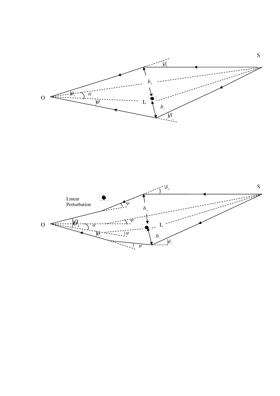
Figure 1: The propagation of light signals from a source to an observer, with a strong gravitational lens in between. The top sketch depicts the situation where the lens is the only disturbance, while in the bottom sketch the effect of a remotely located second mass is also present on the plane of the two rays. The dotted lines represent virtual rays going directly from source and lens to the observer, with the bottom sketch showing how these rays are deflected by the linear perturbation.

3 Time delay anisotropy from a statistical ensemble of galaxies

The analysis in section 1 of light propagation time through a Universe of mass fluctuation could be continued with a calculation of the correlation function between potential gradients, e.g. Eq. (2) for the lowest order form of such a function, by expressing the integral in terms of the matter power spectrum $P(k)$,

$$\langle\nabla^{\prime}_{i}\Phi(\mathbb{r}^{\prime})\nabla^{\prime\prime}_{j}\Phi(\mathbb{r}^{\prime\prime})\rangle=\frac{9\Omega_{m}^{2}H_{0}^{4}}{32\pi^{3}}\int\frac{d^{3}\mathbb{k}}{k^{3}}k_{i}k_{j}e^{i\mathbb{k}\cdot\mathbb{r}}P(k)$$ (3)

where $\mathbb{r}=\mathbb{r}^{\prime}-\mathbb{r}^{\prime\prime}$ and

$$P(k)=\frac{8\pi^{2}}{9\Omega_{m}^{2}H_{0}^{4}}\frac{d}{d\ln k}(\delta\Phi_{k})^{2},$$ (4)

with $\delta\Phi_{k}$ being the standard deviation of the potential over length scales $2\pi/k$.

Now the objective of this paper is to investigate whether time delay measurements can probe the mass distribution in the near ($z\lesssim 1$) Universe where non-linear matter clumping is important, because similar considerations in the context of primordial matter that fills the high redshift Universe have already been made, with the conclusion that such forms of matter causes negligible additional delays (Surpi et al 1996, Bar-kana 1996, Seljak 1994). One could persist with the approach of Eq. (1) by adopting a modified primordial matter spectrum $P(k)$ that includes an ‘extension’ to the non-linear, or large $k$, regime, (Peacock & Dodds 1994, Smith et al 2003), except that concerning the effect of widely spaced and compact clumps on two closely separated light rays it actually makes more sense to calculate directly the time delay induced by the gravitational perturbation of a random ensemble of clumps. This is because of several reasons: (a) while the correlation function of Eq. (3) is relatively simple for the unobservable lowest order term of $\delta\tau$ (i.e. sections 1 and 2) the observable next order term has a much more complex form; (b) the shape of $P(k)$ is unreliable on sub-Mpc scales; (c) the use of a Poisson clump distribution is justified by the ‘nearest neighbour’ interaction phenomenon. More elaborately the differential time delay between two closely spaced rays is due mostly to proximity galaxies located at distances sufficiently small from the two rays in question for mass clustering (or compensation) to exert any significant modification - see below.

Now even if mass correlation over larger scales can be neglected by appealing to Poisson clumps, there still is a form of $P(k)$ to represent this kind of matter inhomogeneity (Eq. 23 of Peebles 1974). Owing to reason (a) above, however, it is much easier to start from first principles. Let us return to the one-way Shapiro time delay when light skirts a mass clump $m$ at ‘impact parameter’ $y$, or more precisely transverse position ${\bf y}$ (with components along the conventional $(0,1,0)$ and $(0,0,1)$ directions, both perpendicular to ${\bf i}={\bf\hat{x}}$) w.r.t. the unperturbed ray, which is

$$\tau=\frac{2Gm}{c^{3}}\ln\left(\frac{4x_{s}x_{ls}}{{\bf y}^{2}}\right),$$ (5)

where $x_{s}$ and $x_{ls}$ are the observer-source and clump-source distance respectively. Take a pair of rays with separation $\delta y\ll y$, the difference in delay between them is

$$\delta\tau = -\frac{2Gm}{c^{3}}\ln\left[\frac{{\bf y}^{2}+2{\bf y}\cdot\delta{\bf y}+(\delta{\bf y})^{2}}{{\bf y}^{2}}\right]$$ (6)

$$= -\frac{2Gm}{c^{3}}\left[\frac{2{\bf y}\cdot\delta{\bf y}}{{\bf y}^{2}}+\frac{(\delta{\bf y})^{2}}{{\bf y}^{2}}-2\left(\frac{{\bf y}\cdot\delta{\bf y}}{{\bf y}^{2}}\right)^{2}-2\frac{{\bf y}\cdot\delta{\bf y}}{{\bf y}^{2}}\frac{(\delta{\bf y})^{2}}{{\bf y}^{2}}+\frac{8}{3}\left(\frac{{\bf y}\cdot\delta{\bf y}}{{\bf y}^{2}}\right)^{3}+\dots\right]$$

If geometry is globally flat, the comoving separation $\delta y$ between the two rays at any position of comoving distance $x$ from the observer O is given by

$$\delta y=x\theta=\frac{xd}{x_{s}},$$ (7)

where $\theta$ is the angle subtended at O by two point sources of distance $d$ apart, both being at the same comoving length $x_{s}$ away from O, to which our two rays map back. These two points could even mark the positions of a pair of strong lensing images, when the light rays associated with the images are perturbed by external mass clumps, in which case $x_{s}=D_{l}$, the distance to the lensing plane, and $\delta\tau$ is the relative delay in the light arrival times between the two images.

The lowest order observable effect is the incoherent contribution to the relative delay between the two rays from each clump, which originates from the second spatial derivative of the clump’s gravitational potential. From section 2 and Eq. (1) we that this is the contribution arising from the $\delta\tau\sim\theta^{2}\sim(\delta y)^{2}$ terms of Eq. (6). In this light, it is clear that only the 2nd and 3rd terms on the right side of Eq. (6) are relevant. Thus, when we square the equation to form the variance, we obtain

$$(\delta\tau_{{\rm incoherent}})^{2}=2\left(\frac{Gm}{c^{3}}\right)^{2}\left[\frac{(\delta{\bf y})^{2}}{{\bf y}^{2}}\right]^{2}+{\rm higher~{}order~{}terms},$$ (8)

where the angle averages employed to go from Eq. (6) to Eq. (8) were $\langle\cos^{2}\vartheta\rangle=$ 1/2 and $\langle\cos^{4}\vartheta\rangle=$ 3/8, with $\vartheta$ being the angle between ${\bf y}$ and $\delta{\bf y}$.

For the rest of this section we shall indeed focus our attention upon one manifestation of shear: the delay in photon arrival times between two strong lensing images. Under this scenario a random walk arises as a result of the two rays skirting all the other clumps on either side of the light path. Their loci then become like two long snakes (Hamana et al 2005, Gunn 1967a,b) as the rays are deflected, largely in tandem, though there is always a small and random relative change in directions, which is the same shear phenomenon as the incoherent relative delay caused by each clump. Both these relative processes of deflection and delay accumulate like $\sqrt{N}$ from one clump to the next if the clump distribution is Poisson, as assumed.

Thus, specifically concerning time delay, as the rays continue their journey the variances $(\delta\tau)_{{\rm incoherent}}^{2}$ from all the clump encounters add, so that to evaluate the total excursion in the arrival time difference one must perform a cylindrical integration with the axis along the $x$-direction. There is however one subtlety here. Since $y$ is the comoving impact parameter its value for deflections at finite $z$ was smaller by by the factor $1+z$. Fortunately this factor cancels out when all the components of the integrand are assembled, though the same does not happen when one computes image distortions by shear, as we shall see. The cumulative variance for a Poisson ensemble of clumps of comoving number density $n$ (i.e. neglecting with caveats the evolution of clump properties, see below) is obtained by an integration down the light path to be

$$[\delta\tau_{{\rm incoherent}}(\mathbb{\theta})]^{2}=2\left(\frac{Gm}{c^{3}}\right)^{2}\int_{0}^{D_{l}}(\delta y)^{4}ndx\int_{y_{{\rm min}}}^{y_{{\rm max}}}\frac{2\pi ydy}{y^{4}}=\frac{2\pi}{5}\left(\frac{Gm}{c^{3}}\right)^{2}\frac{nD_{l}^{5}}{y_{{\rm min}}^{2}}\theta^{4},$$ (9)

if one considers only the contribution to $(\delta\tau)^{2}$ from foreground mass clumps that interact with the light rays during redshifts $z<z_{l}$. In arriving at the final expression of Eq. (9) use was made of Eq. (7). We may get rid of the dependence on $y_{{\rm min}}$ by assuming that it equals the comoving distance at which one or more clumps satisfy the condition $y\leq y_{{\rm min}}$, i.e.

$$y_{{\rm min}}=\frac{1}{\sqrt{\pi nD_{l}}}.$$ (10)

The contribution from background ($z_{l}<z<z_{s}$) clumps may likewise be calculated and included. One would then arrive at a total variance of

$$c^{2}(\delta\tau_{{\rm incoherent}})^{2}=\frac{9}{160}\left(\frac{H_{0}^{4}}{c^{4}}\right)\Omega_{{\rm cl}}^{2}D_{l}^{4}(D_{l}^{2}+D_{ls}^{2})\theta^{4},$$ (11)

after employing the relation $Gnm=\sum_{i}Gn_{i}m_{i}=3H_{0}^{2}\Omega_{{\rm cl}}/(8\pi)$, with $\Omega_{{\rm cl}}$ being the mass density of clumps as a fraction of the critical density.

We intend to pursue an application of the above development, by predicting the effect of external field galaxies on the time delay between strong lensing images, for comparison with observations. Before doing so, however, several remarks about $(\delta\tau)^{2}_{{\rm random}}$ are in order. Apart from the most obvious fact that its final form scales only with one property of the clumps, viz. $\Omega_{{\rm cl}}$, Eq. (11) is valid in the limit $\delta y\ll y$. In terms of the comoving separation $d$ between sources, Eq. (7), this implies (since $\delta y<d$ and $y_{{\rm min}}<y$) that $d\ll y_{{\rm min}}$. Now the images to be used as testbeds have a typical comoving separation $d\lesssim$ 50 kpc, i.e. a scenario under which the criterion is satisfied, because 50 kpc is not much larger than the size of a galaxy. More elaborately, if $y_{{\rm min}}\lesssim d$ one would ‘see’ a galaxy when looking at the sky along any direction: we assume this is not the case.

The next remark is that the sole role played by proximity clumps can be seen from the dependence of $(\delta\tau)^{2}$ on $y_{{\rm min}}$ and not $y_{{\rm max}}$. Thus, on the question of relative time delay caused by galaxies one does not need to take account of large (Mpc scale or more) distances over which mass compensation by galaxy clustering is important. This justifies a posteriori our use of a random clump ensemble without appealing to $P(k)$. It also provides the reason why the effect of voids on the time delay fluctuations can be ignored: since the maximum separation between the two rays is small compared with the typical inter-clump spacing the void-to-void accumulation of the randomly varying second spatial derivative of the void potential function is completely negligible over such distance scales (over much larger (CMB acoustic) distance scales this phenomenon could play a role in lensing deflections via mass clustering, see Holz & Wald 1998, Seljak 1996). The inclusion of void effects will in principle add further signal to the variance $\delta\tau_{{\rm incoherent}}$ for the presently assumed (and justified) Poisson mass distribution, Thus even though the neglected contribution is small, it does mean that our estimate of $\delta\tau_{{\rm incoherent}}$ is conservative.

4 Testing the dynamics of global geometry by strong lensing time delay

The interpretation of cosmological time delay data is usually confined to considerations of the delay within the strong lens system and its immediate environs, with the overall aim of inferring the Hubble constant $H_{0}$ from the observations (Refsdal 1964). If e.g. the lensing mass distribution is a singular isothermal sphere, the relative time delay between two images at angular distances $\theta_{A}$ and $\theta_{B}$ from, and on opposite sides of, the axis of symmetry is given by

$$\Delta\tau_{AB}=\tau_{A}-\tau_{B}=\frac{1+z_{l}}{2}\frac{D_{l}D_{s}}{D_{ls}}(\theta_{A}^{2}-\theta_{B}^{2}),$$ (12)

In Eq. (12) it is assumed, of course, that A and B are images of the same source, usually a time variable background quasar. The Hubble constant clearly affects the delay via the distance dependence, viz. $\Delta\tau_{AB}\sim D_{l}D_{s}/D_{ls}\sim H_{0}^{-1}$ (other cosmological parameters also play a role because $D$ is a multi-dimensional function, but their effects are minor, as noted by Grogin & Narayan 1996). Hence time delay measurements via light curve alignment between images A and B of the quasar, coupled with knowledge of redshifts, can in principle lead to a determination of $H_{0}$.

To date approximately ten strong lensing systems with time delay measurements are available (Saha et al 2006), in each case the delay between two images separated by several arcseconds is typically found to lie within the 10 – 100 days range. One pair of such multiply lensed quasars with similar parameters, SDSS J1004+4112 and HE0435-1223, were reported by Fohlmeister et al 2006 and Kochanek et al 2006 respectively. We shall employ this pair to illustrate how the cosmological distribution of galaxies near the light path can substantially enlarge the random uncertainty in the value of $H_{0}$. For SDSS J1004+4112 where the smallest observed image separation, between images A and B, was $\theta\approx$ 4 arcsec and the comoving distances are $D_{s}=$ 4.77 Gpc, $D_{l}=$ 2.45 Gpc in an $\Omega_{m}=$ 0.3, $\Omega_{\Lambda}=$ 0.7 cosmology, Eq. (11) gives $\delta\tau_{{\rm incoherent}}\approx$ 24 days if we persist with the $\Lambda$CDM standard model by adopting its breakdown of the matter budget to set $\Omega_{{\rm cl}}=$ 0.15 (specifically this assumes that half the baryons, hence approximately the same fraction for dark matter also, of the low $z$ Universe resides in galaxies and their halos, see Fukugita 2004 and Fukugita et al 1998). In fact, taking the above parameters as typical, one could proceed to recast Eq. (11) into a more convenient form:

$$\delta\tau_{{\rm incoherent}}=29.1(h/0.7)^{2}(\Omega_{{\rm cl}}/0.15)(\theta/5~{}{\rm arcsec})^{2}(D_{l}/2.5~{}{\rm Gpc})^{3}\left[1+\left(\frac{D_{ls}}{D_{l}}\right)^{2}\right]^{\frac{1}{2}}~{}~{}{\rm days}.$$ (13)

Since the observed image delay of 38.4 $\pm$ 2.0 days is on par with $\delta\tau_{{\rm random}}$, any estimation of $H_{0}$ that attributes all the observed delay to physics within the strong lens system would have caused this value to vary randomly from the truth by almost 100 %. Other images of SDSS J1004+4112 can also be used as testbeds: the separation of image B from C (also A from D) is $\theta\approx$ 20 arcsec, while the expected time delay between them is $>$ 560 days ($>$ 800 days for A and D), due solely to the strong lens system itself. From Eq. (13) we see that once again $\delta\tau_{{\rm incoherent}}$ is comparable to these delays because of its $\theta^{2}$ scaling.

A repetition of the above analysis to HE0435-1223, where $D_{s}=$ 6.44 Gpc, $D_{l}=$ 1.74 Gpc and $\theta\approx$ 2 arcsec, results in a similar though less drastic conclusion, viz. $\delta\tau_{{\rm incoherent}}\approx$ 4.5 days versus the observed delay of 14.4 $\pm$ 0.8 days. The random error in $H_{0}$ here should then account for an additional fluctuation $\delta H_{0}/H_{0}\approx$ 30 %.

In summary, the distribution, evolution, and mass budget of galaxies as understood in the context of the standard cosmological model leads to the prediction of a random (or incoherent) relative delay between the light arrival times from two images of a strongly lensed background quasar comparable with the observed delay. Since the latter has routinely been interpreted as an effect caused principally by the gravitational field of the lens, and moreover a value of $H_{0}$ is derivable from it if perturbations outside the strong lens are absent, the question of whether additional and hitherto unknown dynamics are responsible for the global flatness of space could be addressed by examining the statistical variation in the $H_{0}$ values that emerge from a large number of strong lensing delay measurements, when such a database becomes available.

If this variation distributes around a value of $H_{0}$ that agrees with other methods of determination, with a standard deviation matching the expectation from Eq. (10), it would imply that for the first time the ensemble gravitational effect of many galaxies spread over cosmological distances has been detected. If, on the other hand, the variation distributes tightly around the accepted value of $H_{0}$ with no room for extra perturbations, the possibility of a new physical phenomenon that complements (even replaces) the law of gravity as the distance scale becomes large must then be inevitable. The fact that there has not been any report of a significant deviation from the $h=$ 0.7 mark in the value of $H_{0}$ as determined by this type of time delay technique may already be pointing to the absence of the random effect discussed here. If this turns out to be really the case, the stability of the global geometry as revealed here would present a serious challenge to cosmology.

We end by pointing out that the possible influence of foreground matter on the measurement of $H_{0}$ was considered in a recent work (Fassnacht et al 2006) under the scenario of this matter being clumped into several foreground groups of galaxies. The present paper, however, calculates for the first time the effect of a random ensemble of many foreground clumps on strong lensing time delay; we then demonstrated that this introduces a large scatter in the resulting value of $H_{0}$. The cause of such a scatter stems mainly from light skirting clumps without passing through them, i.e. cosmological time delay data contain precious information on shear.

References

- (1)
- (2) Bar-Kana, R., 1996, ApJ, 468, 17.
- (3)
- (4) Bennett, C.L. et al 2003, ApJ, 148, 1.
- (5)
- (6) Fassnacht, C.D., Gal, R.R., Lubin, L.M., McKean, J.P., Squires, G.K., Readhead, A.C.S. 2006, ApJ, 642, 30.
- (7)
- (8) Fohlmeister, J. et al 2006, ApJ, submitted (astro-ph/0607513).
- (9)
- (10) Fukugita, M. 2004, in IAU Symp. 220, Dark Matter in Galaxies, ed. S.D. Ryder et al (San Francisco: ASP), 227.
- (11)
- (12) Fukugita, M., Hogan, C.J., & Peebles, P.J.E. 1998, ApJ,503, 518.
- (13)
- (14) Grogin, N.A. & Narayan, R. 1996, ApJ, 464, 92.
- (15)
- (16) Gunn, J.E. 1967, ApJ, 147, 61.
- (17)
- (18) Gunn, J.E. 1967, ApJ, 150, 737.
- (19)
- (20) Hamana, T., Bartelmann, M., Yoshida, N., Pfrommer, C., 2005, MNRAS 356, 829.
- (21)
- (22) Holz, D.E., & Wald, R.M. 1998, PRD, 58, 3501.
- (23)
- (24) Kochanek, C.S., Morgan, N.D., Falco, E.E., McLeod, B.A., Winn, J.N. Dembicky, J., & Ketzeback, B. 2006, ApJ, 640, 47.
- (25)
- (26) Lieu, R. & Mittaz, J.P.D. 2007, ApJ in press (astro-ph/0608587).
- (27)
- (28) Peacock, J.P. & Dodds, S.J. 1994, MNRAS, 267, 1020.
- (29)
- (30) Peebles, P.J.E. 1974, A & A, 32, 197.
- (31)
- (32) Refsdal, S. 1964, MNRAS, 128. 307.
- (33)
- (34) Saha, P., Coles, J., Maccio’, A.V., & Williams, L.L.R., 2006, ApJ, 650, L17.
- (35)
- (36) Seljak, U. 1996, ApJ, 463, 1.
- (37)
- (38) Seljak, U. 1994, ApJ, 436, 509.
- (39)
- (40) Smith, R.E., Peacock, J. A., Jenkins, A., White, S. D. M., Frenk, C. S., 2003, MNRAS 341, 1311.
- (41)
- (42) Spergel, D. et al 2007, ApJ in press (astro-ph/0603449).
- (43)
- (44) Surpi, G.C., Harari, D.D., Frieman, J.A. 1996, ApJ, 464, 54.
- (45)