The globular cluster NGC 1978 in the Large Magellanic Cloud

Abstract

We have used deep high-resolution Hubble Space Telescope ACS observations to image the cluster NGC 1978 in the Large Magellanic Cloud. This high-quality photometric data set allowed us to confirm the high ellipticity ($\epsilon\sim$0.30$\pm$0.02) of this stellar system. The derived Color Magnitude Diagram allowed a detailed study of the main evolutionary sequences: in particular we have detected the so called Bump along the Red Giant Branch (at $V_{555}$=19.10$\pm$0.10). This is the first detection of this feature in an intermediate-age cluster.
Moreover the morphology of the evolutionary sequence and their population ratios have been compared with the expectations of different theoretical models (namely BaSTI, PEL and Padua) in order to quantify the effect of convective overshooting. The best agreement (both in terms of morphology and star counts) has been found the PEL (Pisa Evolutionary Library) isochrone with Z=0.008 (consistenly with the most recent determination of the cluster metallicity, [M/H]=-0.37 dex) and a mild overshooting efficiency ($\Lambda_{os}$=0.1). By adopting this theoretical set an age of $\tau$=1.9$\pm$0.1 Gyr has been obtained.

1 Introduction

The Large Magellanic Cloud (LMC) is the nearest galaxy of the Local Group with evident star formation activity. The LMC has a very popolous system of globular clusters that covers a large range of metallicities and ages (see Olszewski, Suntzeff & Mateo (1996) and references therein). We can distinguish an old population, coeval with the Galactic globular cluster (GGC) system, an intermediate (1-3 Gyr) and a young population, ranging from a few million years to 1 Gyr. Hence the stellar populations of the LMC cluster system represent an important laboratory to study and test stellar evolution models in a different age-regime with respect to the Galactic system.

The first surveys devoted to study the properties of these clusters have been carried out in the optical (van den Bergh, 1981) and in the near-infrared (Persson et al., 1983) spectral range and were based on measurements of their integrated colours (Searle, Wilkinson, & Bagnuolo, 1980; Elson & Fall, 1985). However, only in the last decade the main properties of the resolved stellar populations in LMC globulars have been investigated by means of high resolution photometry of individual stars (Vallenari et al., 1994; Corsi et al., 1994; Ferraro et al., 1995; Brocato et al., 2001; Mackey & Gilmore, 2003; Ferraro et al., 2004; Mucciarelli et al., 2006). These works have produced a number of interesting results: (i) the oldest clusters of the LMC are coeval with GGCs (Testa et al., 1995; Brocato et al., 1996; Olsen et al., 1998; Mackey & Gilmore, 2004). The recent census of the old LMC globulars presented by Mackey & Gilmore (2004) counts a total of 15 objects with ages $\geq$ 10 Gyr; (ii) the dominant population is constituted of $\sim$100 young and intermediate age clusters, with ages $<$3 Gyr; (iii) the absence of objects in the huge age range from $\sim$3 to $\sim$ 13 Gyr (the so-called Age Gap): The Age Gap problem has been largely investigated (see i.e. Bekki et al., 2004) and clusters in the Age Gap actively searched (Geisler et al., 1997; Rich et al., 2001; Mackey et al., 2006), however up to date, only one candidate, namely ESO 121-SC03, possibly falls in such an age range. In spite of these efforts, the overall formation history of the LMC is still an open issue, since a firm age-metallicity relation (AMR) has not been established, yet. Indeed, homogeneous and accurate metallicities and ages for a significant sample of LMC clusters are mandatory to derive a reliable AMR.

Accurate ages from the measurement of the Main-Sequence (MS) Turn-Off (TO) region are still sparse and very model (i.e. isochrones) dependent. The only homogeneous age-scale available still relies on the so called s-parameter (Elson & Fall, 1985, 1988), an empirical quantity related to the position of the cluster in the dereddened (U-B) vs (B-V) color-color diagram. This parameter linearly correlates with the logarithm of the age (Elson & Fall, 1985; Girardi et al., 1995).

Most chemical abundance determinations for LMC clusters are based on low-resolution spectra (Olszewski et al., 1991), integrated infrared spectroscopy (Oliva & Origlia, 1998) or photometric techniques (Dirsch et al., 2000; Larsen et al., 2000). Detailed chemical abundances from high-resolution spectra are still sparse (Hill et al., 2000; Johnson et al., 2006; Ferraro et al., 2006).

With the ultimate goal of constructing a homogeneous age-metallicity scale for the LMC clusters, we started a program which makes use of the last generation of instruments (imager and multi-object spectrograph) in order to perform an appropriate study of stellar population, age, metal content and structural parameters for a number of pillar clusters. In this paper we present the results for one of the most massive and luminous globulars in the LMC, namely NGC 1978. This cluster has been considered for years a peculiar object (i) because of its high-ellipticity ($\epsilon$=0.3, Fischer et al., 1992), significantly larger than the one typically measured in stellar clusters (Goodwin, 1997), and (ii) because it has been suspected to harbour a chemically inhomogeneous stellar population (Alcaino et al., 1999; Hill et al., 2000). However, Ferraro et al. (2006) has recently presented high resolution spectra for eleven giants in this cluster, obtaining [Fe/H]=-0.38 dex, with a very low dispersion ($\sigma$=0.07 dex), firmly excluding the presence of a significant metallicity spread in this cluster. Here we present a high precision CMD of the cluster based on observations obtained with the Advanced Camera for Surveys (ACS) on board the Hubble Space Telescope (HST). The morphology and the population ratios along the main evolutionary sequences have been used to quantify the effect of convective overshooting. Finally, by combining the precise measure of the MS-TO with accurate estimate of the cluster metallicity (Ferraro et al., 2006) we also provide an accurate estimate of the cluster age.

2 Observations and data analysis

2.1 Observations

The photometric dataset consists of high-resolution images obtained with ACS@HST (300 sec and 200 sec long) through the F555W and F814W filters. These images have been retrieved from ESO/ST-ECF Science Archive (Proposal ID 9891, Cycle 12). The observations have been obtained with the Wide Field Channel (WFC) that provides a field of view of $\approx$200” $\times$200” with a plate scale of 0.05 arcsec/pixel. The WFC is a mosaic of two CCDs, both with 4096$\times$2048 pixels separated by a gap of $\sim$50 pixels. The first chip has been centered on the cluster center, while the second chip sampled a contiguos field. All images were reduced with the ACS/WFC pipeline, in order to perform bias and dark subtractions and flatfield correction. The photometric reduction was performed by using the DAOPHOT-II (Stetson, 1987) Point Spread Function (PSF) fitting method. The output catalog includes about 40,000 objects from the first chip and more than 10,000 from the second chip and it has been calibrated in the ACS/WFC Vega-mag system, following the prescriptions of Bedin et al. (2005). Finally, the ACS catalog has been astrometrized in the 2MASS astrometric system by matching the IR catalog presented in Mucciarelli et al. (2006).

2.2 The Color-Magnitude Diagram

Fig. 1 shows the calibrated color-magnitude diagram (CMD) for the chip centered on the cluster. Stars in the brightest portion of the Giant Branches could be saturated and/or in the regime of non linearity of the CMD. Hence for stars brighter than $V_{555}$=17.6 (this magnitude level is marked with an horizontal dashed line in Fig. 1), magnitudes, colours and level of incompleteness are not safely measured. This CMD (reaching the magnitude limit of $V_{555}\sim$26) shows the typical evolutionary features of an intermediate-age stellar population, namely:

(1) the brightest portion of the MS at $V_{555}<$21 shows a hook-like shape, typical of the evolution of intermediate-mass stars ( $M>1.2M_{\odot}$ ) which develop a convective core . In particular, the so-called overall contraction phase (Salaris & Cassisi, 2006) is clearly visible between the brightest portion of the MS and the beginning of the Sub-Giant Branch (SGB) at $V_{555}\sim$20.9.

(2) the SGB is a narrow, well-defined sequence at $V_{555}\sim$20.7, with a large extension in color ($\delta(V_{555}$-$I_{814})$ $\sim$0.6 mag). The blue edge of the SGB is broad and probably affected by blending, especially in the most internal region of the cluster.

(3) the Red Giant Branch (RGB) is fully populated; this is not surprising since this cluster has already experienced the RGB Phase Transition (see the discussion in Ferraro et al. (2004) and Mucciarelli et al. (2006)).

(4) the He-Clump is located at $V_{555}\sim$19.1 and $(V_{555}-I_{814})\sim$1.15.

Fig. 2 shows the CMD of the external part of the ACS@HST field of view (corresponding to r$>$140” from the cluster center). This CMD can be assumed as representative of the field population surrounding the cluster. In particular, the CMD shows two main components:

(1) a blue sequence extended up to $V_{555}\sim$17.

(2) a SGB which merges into the MS at $V_{555}\sim$22.2, corresponding to a population of $\approx$5 Gyr. We interpret this feature as a signature of the major star-formation episode occurred 5-6 Gyr ago, when LMC and Small Magellanic Cloud (SMC) were gravitationally bounded (Bekki et al., 2004).

2.3 Completeness

In order to quantify the degree of completeness of the final photometric catalog, we used the well-know artificial star technique (Mateo, 1988), and simulated a population of stars in the same magnitude range covered by the observed CMD (excluding stars brighter than $V_{555}$=17.6, corresponding to the saturation level) and with $(V_{555}-I_{814})\sim$0.8 mean color. The artificial stars have been added to the original images and the entire data reduction procedure has been repeated using the enriched images. The number of artificial stars simulated in each run ($\sim$ 2,000) are a small percentage ($\sim$5%) of the detected stars, hence they cannot alter the original crowding conditions. A total of $\sim$250 runs were performed and more than 500,000 stars have been simulated. In order to minimize the effect of incompleteness correction, we have excluded the very inner region of the cluster (r$<$20”, where the crowding conditions are most severe) from our analysis. In Fig. 3 the completeness factor $\phi=\frac{N_{rec}}{N_{sim}}$ (defined as the fraction of recovered stars over the total simulated ones) is plotted as a function of the $V_{555}$ magnitude in two different radial regions, namely between 20” and 60” and at r$>$60” from the cluster center, respectively.

2.4 The RGB-Bump

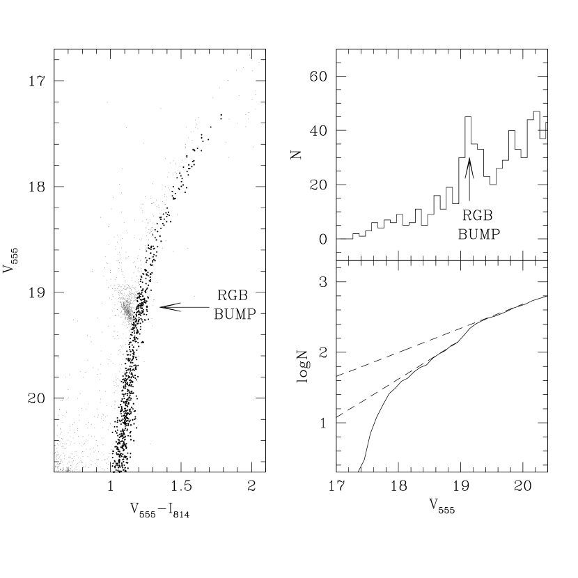
Figure 4: Left: the bright portion of the CMD of NGC 1978 (grey points) with the selected RGB stars (black points). The arrow indicates the magnitude of the RGB Bump. Right: differential (upper panel) and integrated (lower panel) LFs, computed for the RGB stars, excluding the He-Clump and AGB populations. The arrow in the upper panel indicates the position of the RGB Bump. The dashed lines in the lower panel are the linear fit to the regions above and below the RGB Bump.

The extended and populated RGB in NGC 1978 gives the possibility to search for the so-called RGB-Bump. This is the major evolutionary feature along the RGB. It flags the point when the H-burning shell reaches the discontinuity in the H-abundance profile left by the inner penetration of the convection. This feature has been predicted since the early theoretical models (Iben, 1968) but observed for the first time in a globular cluster almost two decades later (King et al., 1984). Since that first detection the RGB-Bump was identified in several GGCs (Fusi Pecci et al., 1990; Ferraro et al., 1999; Zoccali et al., 1999) and in a few galaxies in the Local Group (Sextant (Bellazzini et al., 2001), Ursa Minor (Bellazzini et al., 2002), Sagittarius (Monaco et al., 2002)). Accordingly with the prescriptions of Fusi Pecci et al. (1990), we have used the differential and integrated luminosity function (LF) to identify the magnitude level of the RGB-Bump in NGC 1978. In doing this, we have (1) selected stars belonging to the brightest ($V_{555}<$20.6) portion of the RGB; (2) carefully excluded the bulk of the He-Clump and AGB stars by eye; (3) defined the fiducial ridge line for the RGB, rejecting those stars lying at more than 2$\sigma$ from the ridge line. Fig. 4 shows the final RGB sample (more than 600 stars) and both the differential and integrated LFs. The RGB-Bump appears in the differential LF as a well defined peak at $V_{555}^{bump}=19.10$ and it is confirmed in the integrated LF as a evident change in the slope.

For both LFs the assumed bin-size is 0.1 mag; in order to check the uncertainty in the Bump magnitude level, we have tested the position of this feature by using LFs computed with different binning. The impact of the selected bin-size is not crucial: a difference of 0.2 mag corresponds to a variation $<$0.05 mag in the detection of RGB Bump. By considering the intrinsecal width of the peak in differential LF, we estimate a conservative error $<$0.10 mag.

Finally, we note that the RGB Bump is brighter and reddest than of the bulk of the He-Clump and the latter merges into the RGB at faintest magnitude ($V_{555}\sim$19.3, see Fig. 4; hence the possibility of contamination is negligible.

3 The cluster ellipticity

Most globular clusters in the Galaxy show a nearly spherical shape, with a mean ellipticity $\epsilon$=0.07 (White & Shawl, 1987) and more than 60% with $\epsilon<$0.10. One of the most remarkable exception is represented by $\omega$ Centauri that is clearly more elliptical than the other GGCs: its ellipticity is $\epsilon$=0.15 in the external regions with a evident decrease in the inner regions, with $\epsilon$=0.08 (Pancino et al., 2003). Conversely, the LMC clusters (as well as those in the SMC) show a stronger departure from the spherical simmetry. Geisler & Hodge (1980) estimated the ellipticities of 25 popolous LMC clusters, finding a mean value of $\epsilon$=0.22; Goodwin (1997) obtained a lower average value for the LMC clusters ($\epsilon$=0.14), but still higher than the mean ellipticity of the GGCs. Moreover, in the LMC the presence of many double or triple globular clusters has been interpretated as a clue of the possibility of merger episodes between subclusters with the result to create stellar clusters with high ellipticities (Bhatia et al., 1991).
Previous determinations (Geisler & Hodge, 1980; Fischer et al., 1992) suggested large values of ellipticity for NGC 1978.

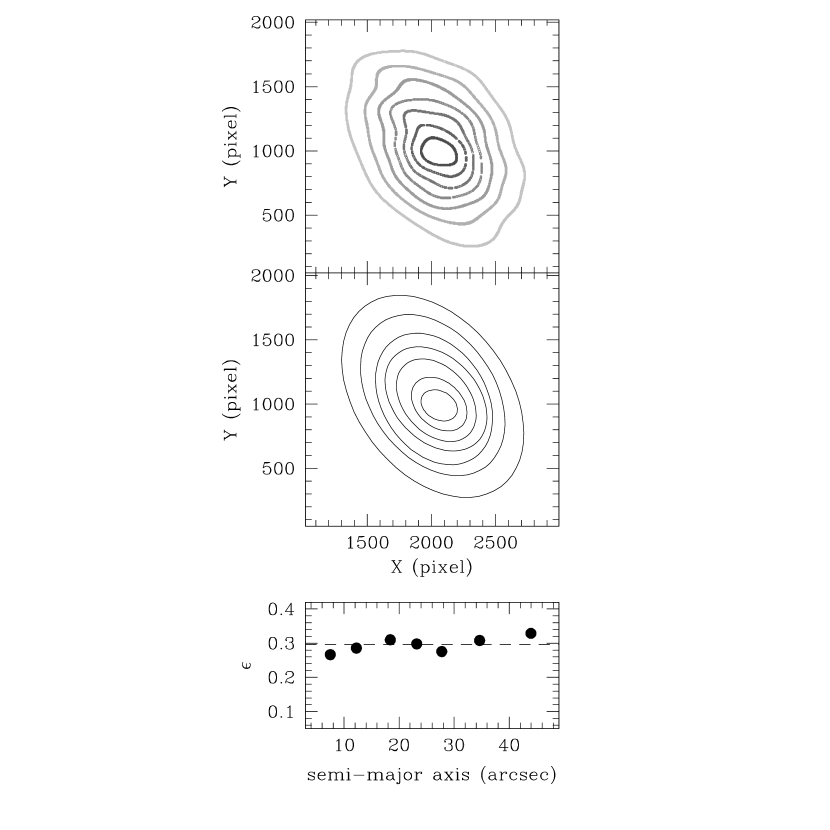
Figure 5: Upper panel: the map of NGC 1978 with the isodensity contours; central panel: the best fit ellipses of the isodensity contours; lower panel: ellipticity of the best fit ellipses as a function of the semi-major axis in arcsecond. The horizontal dashed line indicate the mean value.

We have used the ACS catalog to derive a new measurement of the ellipticity of the cluster, in doing this we computed isodensity curves and adopting an adaptive kernel technique, accordingly to the prescription of Fukunaga (1972). In doing this we have adopted the center of gravity of the cluster computed using the near-infrared photometry obtained with SOFI (Mucciarelli et al., 2006). The isodensity curves have been computed using all the stars in the first chip with $V_{555}<$22 (approximately two magnitudes below the TO region) in order to minimize the incompleteness effects . Finally, we have fitted the isodensity curves with ellipses. Fig. 5 shows the cluster map with the isodensity contours (upper panel), the corresponding best fit ellipses (central panel) and their ellipticity as a function of the semi-major axis in arcsecond (lower panel). No evidence of subclustering or double nucleus is found. The average value of the ellipticity results $\epsilon$=0.30 (with a root mean square of 0.02), without any radial trend. This value is in good agreement with the previous estimates (Geisler & Hodge, 1980; Fischer et al., 1992) and confirms the surprisingly high ellipticity of NGC 1978.

4 The cluster age

The determination of the age of a stellar population requires an accurate measure of the MS TO and the knowledge of the distance modulus, reddening and overall metallicity. For NGC 1978 we used the recent accurate determination of [Fe/H]=-0.38$\pm 0.02$ dex (Ferraro et al., 2006) and $<[\alpha/Fe]>$ almost solar (Mucciarelli et al., in preparation), based on high-resolution spectra, to derive the overall metallicity [M/H]. In doing this, we adopted the relation presented by Salaris et al. (1993):

$$[M/H]\sim[Fe/H]+\log{(0.694\cdot 10^{<[\alpha/Fe]>}+0.306)},$$

obtaining [M/H]$\sim$ -0.37 dex.
In the case of intermediate age stellar systems, the measurements of the age is complicated by the presence of a convective core, whose size needs to be parametrized ($\Lambda_{os}$) . We then use different sets of theoretical isochrones with different input physics, in order to study the impact of the convective overshooting in reproducing the morphology of the main evolutionary sequences in the CMD.

• BaSTI models: BaSTI ( A Bag of Stellar Tracks and Isochrones) evolutionary code described in Pietrinferni et al. (2004) computes isochrones with and without the inclusion of overshooting. The overshoot efficiency depends on the stellar mass: (1) $\Lambda_{os}$=0.2 for masses larger than 1.7 $M_{\odot}$; (2) $\Lambda_{os}=0.25\cdot(M/M_{\odot}-0.9)$ for stars in the 1.1-1.7 $M_{\odot}$ range; (3) $\Lambda_{os}$=0 for stars less massive than 1.1 $M_{\odot}$.
  

• Pisa models : PEL (Pisa Evolutionary Library, Castellani et al. (2003)) provides an homogeneous set of isochrones computed without overshooting and with two different values of $\Lambda_{os}$, namely 0.1 and 0.25.
  

• Padua models : in these isochrones (Girardi et al., 2000) $\Lambda_{os}^{Padua}$=0 for stars less massive than 1 $M_{\odot}$, where the core is fully radiative. The overshooting efficiency has been assumed to increase with stellar mass, according to the relation $\Lambda_{os}^{Padua}=M/M_{\odot}-1$ in the 1-1.5 $M_{\odot}$ range; above 1.5 $M_{\odot}$ a costant value of $\Lambda_{os}^{Padua}$=0.5 is assumed. Note that this value corresponds to $\Lambda_{os}\sim$ 0.25 in the other models, where the extension of the convective region (beyond the classical boundary of the Schwarzschild criterion) is measured with respect to the convective core border.
  

4.1 The morphology of the evolutionary sequences

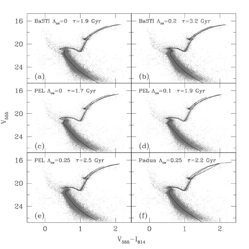
Figure 6: Best-fit theoretical isochrones overplotted to the observed CMD of NGC 1978 (only stars at r$>$20” from the cluster center are plotted) obtained with theoretical isochrones: each panel shows a different model and the corresponding $\Lambda_{os}$ value and age. Reddening and distance moduli for each model are reported in Table 1.

From each set of theoretical models, we selected isochrones with Z=0.008 (corresponding to [M/H]=-0.40 dex), consistent with the overall metallicity of the cluster and we assumed a distance modulus $(m-M)_{0}\sim$18.5 (van den Bergh, 1998; Clementini et al., 2003; Alves, 2004) and E(B-V)=0.10 (Persson et al., 1983). However, in order to obtain the best fit to the observed sequences with each isochrone set, we left distance modulus and reddening to vary by $<|$10$|$% and $<|$30$|$% , respectively. Fig. 6 shows the best fit results for each isochrone set, while Table 1 lists the corresponding best fit values of age, reddening, distance modulus and the predicted magnitude level for the RGB-Bump. The best fit solution from each model set has been identified as the one matching the following features: (i) the He-Clump magnitude level, (ii) the magnitude difference between the He-Clump and the SGB and (iii) the color extension of the SGB. The theoretical isochrones have been reported into the observational plane by means of suitable transformations computed by using the code described in Origlia & Leitherer (2000) and convolving the model atmospheres by Bessel, Castelli & Plez (1998) with the ACS filter responses. In the following, we briefly discuss the comparison between the observed evolutionary features and theoretical predictions.

• BaSTI models: By selecting canonical models from the BaSTI dataset, the best fit solution gives an age of 1.9 Gyr, with E(B-V)=0.09 and a distance modulus of 18.47. Despite of the good matching of the He-Clump and SGB magnitude level, and the RGB slope, this isochrone does not properly reproduce the shape of the TO region and the overall contraction phase (panel (a) of Fig.6). The best-fit solution from overshooting models gives an age of 3.2 Gyr, $(m-M)_{0}$= 18.43 and E(B-V)=0.09, and matches the main loci of the evolutionary sequences in the CMD. In particular, this isochrone provides a better match to the hook-like region (between the MS and the SGB, see panel (b) of Fig.6).
  

• PEL models: Panels (c), (d) and (e) of Fig. 6 show the best fit solutions obtained by selecting 3 different $\Lambda_{os}$. In all cases $(m-M)_{0}$=18.5 and E(B-V)=0.09 are used. As can be seen values of $\Lambda_{os}$=0 and $\Lambda_{os}$=0.25 isochrones fail to fit the SGB extension and the hook-like feature, conversely a very good fit is obtained with a mild-overshooting ($\Lambda_{os}$=0.1) and an age of $\tau$=1.9 Gyr.
  

• Padua models: The best-fit solution gives $\tau$=2.2 Gyr, $(m-M)_{0}$=18.38 and E(B-V)=0.07 ( Panels (f) of Fig. 6). This isochrone well-reproduces the complex structure of the TO and the core contraction stage, as well as the SGB structure and the RGB slope. However, it requires distance modulus and reddening significantly lower than those generally adopted for the LMC.

From this comparison, it turns out that only models with overshooting are able to best fit the morphology of the main evolutionary sequences in the observed CMD. In particular, the best fit solutions have been obtained with the BaSTI overshooting model with $\tau$=3.2 Gyr, the PEL mild-overshooting model ($\Lambda_{os}$=0.1) and $\tau$=1.9 Gyr and the Padua model with $\Lambda_{os}^{Padua}$=0.25 (corresponding to $\Lambda_{os}$=0.25) and $\tau$=2.2 Gyr.

However, it must be noted that none of these models satisfactorly can fit the observed Bump level, the BaSTI and Padua models being $\approx$0.1 and 0.3 mag fainter, respectively, and the PEL model $\approx$0.2 mag brighter, perhaps suggesting that evolutionary tracks for stars with M$>$1$M_{\odot}$ still need some fine tuning to properly reproduce the luminosity of this feature.

4.2 Population ratios

Since the comparison between the observed CMD and theoretical isochrones is somewhat qualitative, we also performed a quantitative comparison between theoretical and empirical population ratios: this yields a direct check of the evolutionary timescales. To do this, we define four boxes selecting the stellar population along the main evolutionary features in our CMD, namely the He-Clump, the SGB, the RGB (from the base up to $V_{555}\sim$19.4) and finally the brightest ($\sim$ 1 mag) portion of the MS; these boxes are show in Fig. 7, overplotted to the cluster CMD. Star counts in each box have been corrected for incompleteness, by dividing the observed counts by the $\phi$ factor obtained from the procedure described in Sec. 2.3 (see also Fig. 3) for each bin of magnitude.

Star counts have been also corrected for field contamination. To estimate the degree of contamination by foreground and background stars we have applied a statistical technique. We have used the CMD shown in Fig. 2 as representative of the field population. The number of stars counted in each box in the control field have been normalized to the cluster sampled area and finally subtracted from the cluster star counts. The final star counts per magnitude bin in each box have been estimated accordingly to the following formula:

$$N_{corr}=\frac{N_{obs}}{\phi}-N_{field},$$

where ${N_{obs}}$ are the observed counts and $N_{field}$ the expected field star counts. We find $N_{MS}$=4331, $N_{SGB}$=632, $N_{RGB}$=450 and $N_{He_{Cl}}$=311, where $N_{MS}$, $N_{RGB}$, $N_{SGB}$ and $N_{He-Cl}$ are the number of stars in the box as sampling the MS, the RGB, the SGB and the He-Clump population, respectively.

Uncertainties in the computed population ratios have been estimated using the following formula

$$\sigma_{R}=\frac{\sqrt{R^{2}\cdot\sigma_{D}^{2}+\sigma_{N}^{2}}}{D}$$

where $R=N/D$ is a given population ratio, N is the numerator and D the denominator of the ratio. The errors $\sigma_{N}$ and $\sigma_{D}$ for any population have been assumed to follow a Poisson statistics. In addition, in the error budget we also include the uncertainty due to the positioning of the box edges: note that a slightly different($\pm 1\sigma$) assumption in the definition of the box edge has little impact (typically 7-8%) on the star counts. This uncertainty has been quadratically added to the Poissonian error.

On the basis of the boxes shown in Fig. 7 we defined four population ratios , as listed in Table 2: (i) $N_{RGB}$/$N_{SGB}$; (ii) $N_{RGB}$/$N_{He-Cl}$; (iii) $N_{SGB}$/$N_{He-Cl}$; (iv) $N_{MS}$/$N_{(SGB+RGB)}.$ For each selected model, corresponding theoretical population ratios have been estimated by convolving the isochrone set shown in Fig.4 with an Initial Mass Function (IMF), according with the prescriptions of Straniero & Chieffi (1991). In order to check the sensitivity of the population ratios to the adopted IMF, we have used three different values for the IMF slope $\alpha$: 2.35 (Salpeter, 1955), 2.30 (Kroupa, 2001) and 3.5 (Scalo, 1986) at M$>$1$M_{\odot}$. In the considered mass range (between 1 and 2 $M_{\odot}$), the theoretical population ratios are poorly dependent on the assumed IMF, with a 16% maximum variation (between Scalo and Kroupa IMFs) for the $N_{MS}$/$N_{(SGB+RGB)}$ ratios. Hence in the following the population ratios are computed by using a Salpeter IMF.

As results, we found that BaSTI and PEL canonical models predict a lower (by $<$40%) of the $N_{MS}$/$N_{(SGB+RGB)}$ and higher $N_{RGB}$/$N_{He-Cl}$ and $N_{SGB}$/$N_{He-Cl}$ (by $<$35% and $<$100%, respectively) population ratios with respect to the observed ones. Isochrones with high overshooting ($\Lambda_{os}$=0.2-0.25) show an opposite trend, with higher (by $<$50%) $N_{MS}$/$N_{(SGB+RGB)}$ and lower (by $<$30%) $N_{RGB}$/$N_{He-Cl}$ and $N_{SGB}$/$N_{He-Cl}$ ratios. The isochrone with $\Lambda_{os}$=0.1 from PEL dataset reasonably reproduces all the population ratios. Only the $N_{MS}$/$N_{(SGB+RGB)}$ ratio turns out to be $\sim$15% lower than the observed one.
We conclude that the best agreement with observations (both in terms of evolutionary sequence morphology and star counts) has been obtained by using PEL models computed with a mild overshooting ($\Lambda_{os}$=0.1) and $\tau$=1.9 Gyr. Also, the required values of distance modulus and reddening are fully consistent with those generally adopted for NGC 1978. In order to estimate the overall age uncertainty, we took into account the major error source, namely the distance modulus. Hence, we have repeated the best-fitting procedure by using the PEL isochrones with mild-overshooting, and varying the distance modulus by $\pm$0.05 and $\pm$0.1 mag with respect to the reference value of 18.5. A variation of $\pm$0.05 mag still allows a good fit of the CMD features with isochrones within $\mp$0.1 Gyr from the reference value of 1.9 Gyr. A variation of $\pm$0.1 mag in the distance modulus, does not allows to simultaneously fit the He-Clump magnitude level and the extension of SGB, whatever age is selected. Hence, we can assign a formal error of $\pm$0.1 Gyr to our age estimate.

5 Discussion and Conclusions

The photometric analysis of the ACS-WFC CMD of NGC 1978 presented here provided three major results, that can be summarized as follows: i) the firm detection of the RGB Bump at $V_{555}$=19.10$\pm$0.10, ii) a new, independent estimate of the cluster ellipticity ($\epsilon$=0.30$\pm$0.02) and iii) an accurate measure of the cluster age ($\tau$=1.9$\pm$0.1 Gyr).

The detection presented here is the first clearcut detection of the RGB Bump in an intermediate age cluster and it confirms the theoretical expectation that this feature also occurs in relatively massive stars (the estimated TO mass for this cluster is $\sim$1.5 $M_{\odot}$, see Tab. 1). Note that this result opens the possibility to study the behaviour of the RGB Bump as a function of the cluster age and it provides crucial insight on the internal structure of intermediate mass stars.

The high-ellipticity ($\epsilon$=0.30$\pm$0.02) of NGC 1978 poses two major questions: i) why the LMC clusters in general, and NGC 1978 in particular, are, in average, more elliptical than those in the Milky Way? ii) why NGC 1978 is more elliptical than the other LMC clusters?
Goodwin (1997) suggests that the relatively small LMC tidal field can preserve the pristine triaxial structure of the clusters, while the strong tidal field of our Galaxy tend to destroy it, thus removing at least part of the ellipticity.
In order to explain the especially high ellipticity of NGC 1978 three main hypothesis have been proposed in the past: a merging episode, a rotation effect and an anisotropic velocity dispersion tensor (Fischer et al., 1992). The merging scenario has been proposed because the broad RGB from ground-based BVRI photometry (Alcaino et al., 1999) and because the preliminary evidence of a metallicity dispersion from high-resolution spectroscopy of two RGB stars (Hill et al., 2000) ($\delta$[Fe/H]$\sim$0.2-0.3 dex). However, the tiny RGB sequence presented in this work as well as the recent iron abundance estimate from high-resolution spectra of eleven RGB stars presented by Ferraro et al. (2006) definitely excluded any significant metallicity spread within the cluster.

Our new age estimate ($\tau$=1.9$\pm$0.1 Gyr) of NGC 1978, coupled with the new iron abundance determination ([Fe/H]=-0.38$\pm$0.02 dex) by Ferraro et al. (2006), provide new coordinates for this cluster in the age-metallicity plane. This is especially important, since the correct shape of the AMR in the LMC is still matter of debate: in particular the origin of the observed bimodality in the LMC cluster age distribution has been interpreted as the evidence for two major episodes of star formation. Pagel & Tautvaisiene (1998) computed two different AMR semi-empirical models for the LMC, with a continuous star formation and with two burst episodes occurred $\sim$14 and 3 Gyr ago, respectively. Fig. 8 shows the results of these theoretical predictions. For comparison, the position of NGC 1978 in the age-metallicity diagram based on i) old metallicity ($\rm-0.6<[Fe/H]<-0.4$ Olszewski et al. (see 1991); de Freitas Pacheco, Barbuy & Idiart (see 1998)) and age (2-3.3 Gyr Olszewski, 1984; Geisler et al., 1997; Girardi et al., 1995) estimates (grey box), ii) the iron abundance by Hill et al. (2000) and age by Bomans et al. (1995) (open square), and finally iii) the most recent metallicity by Ferraro et al. (2006) and age from the present work (big black dot) are shown. It is interesting to note that old coordinates (grey box) barely fit with the bursting scenario, while the more recent measurements by Hill et al. (2000) place the cluster far below any model. Our new coordinates are somewhat consistent with both the proposed star formation scenarios.
Similar accurate ([Fe/H], $\tau$) coordinates for a significant number of LMC clusters with different ages and metallicities are urgently needed to disentagle different formation scenarios. This is the aim of our ongoing global project. By combining detailed chemical abundance (from high-resolution spectra) and ages (from high quality photometry) to a number of pillar LMC clusters, we plan to calibrate a suitable age and metallicity scale for the entire LMC globular cluster system, with the ultimate goal of providing a robust AMR.

Table 1: Age, distance modulus, reddening , Turn-Off mass and magnitude level of the RGB-Bump from best-fit BaSTI, PEL and Padua isochrones.

	BaSTI	BaSTI	PEL	PEL	PEL	PADUA
	$\Lambda_{os}$=0	$\Lambda_{os}$=0.2	$\Lambda_{os}$=0	$\Lambda_{os}$=0.1	$\Lambda_{os}$=0.25	$\Lambda_{os}$=0.25
Age (Gyr)	1.9	3.2	1.7	1.9	2.5	2.2
$(m-M)_{0}$	18.47	18.43	18.50	18.50	18.50	18.38
E(B-V)	0.09	0.09	0.09	0.09	0.09	0.07
$M_{TO}$ ($M_{\odot}$)	1.47	1.45	1.49	1.49	1.44	1.45
$V_{555}^{Bump}$	19.10	19.22	18.73	18.88	19.39	19.44

Table 2: Theoretical population ratios from BaSTI, PEL and Padua best-fit isochrones, and corresponding observed ratios for NGC 1978.

Population Ratio	BaSTI	BaSTI	PEL	PEL	PEL	PADUA	Observed
	$\Lambda_{os}$=0	$\Lambda_{os}$=0.2	$\Lambda_{os}$=0	$\Lambda_{os}$=0.1	$\Lambda_{os}$=0.25	$\Lambda_{os}$=0.25
MS/(RGB+SGB)	2.40	6.05	2.10	3.27	7.06	6.92	4.00$\pm$0.40
SGB/He-Cl	4.16	1.63	4.90	2.01	1.62	1.05	2.03$\pm$0.22
RGB/He-Cl	1.95	1.07	2.41	1.64	1.03	0.78	1.45$\pm$0.19
RGB/SGB	0.58	0.65	0.49	0.81	0.64	0.75	0.71$\pm$0.10
$SGB_{s}$/He-Cl	1.39	0.64	1.43	0.85	0.61	0.36	1.12$\pm$0.12
MS/(RGB+$SGB_{s}$)	4.14	9.61	4.00	4.75	11.43	11.29	5.43$\pm$0.42

Figure 1: (V, V-I) CMD of the LMC cluster NGC 1978, obtained with ACS@HST (only first chip). The dashed line indicates the saturation level.

Figure 2: (V, V-I) CMD of the outer region (r$>$140” from the cluster center) of NGC 1978, as obtained with ACS@HST (only second chip).

Figure 3: Completeness curves computed in two radial sub-regions of NGC 1978. The black points indicate the value of the $\phi=\frac{N_{rec}}{N_{sim}}$ parameter calculated for each magnitude bin. The completeness curves have been computed for $V_{555}<$17.6, corresponding to the saturation level. Tipycal errorbars are also indicated.

Figure 7: The bright portion of the NGC 1978 CMD (only stars at r$>$20” from the cluster center are plotted) with the selection boxes adopted to sample the MS, SGB, RGB and He-Clump populations.

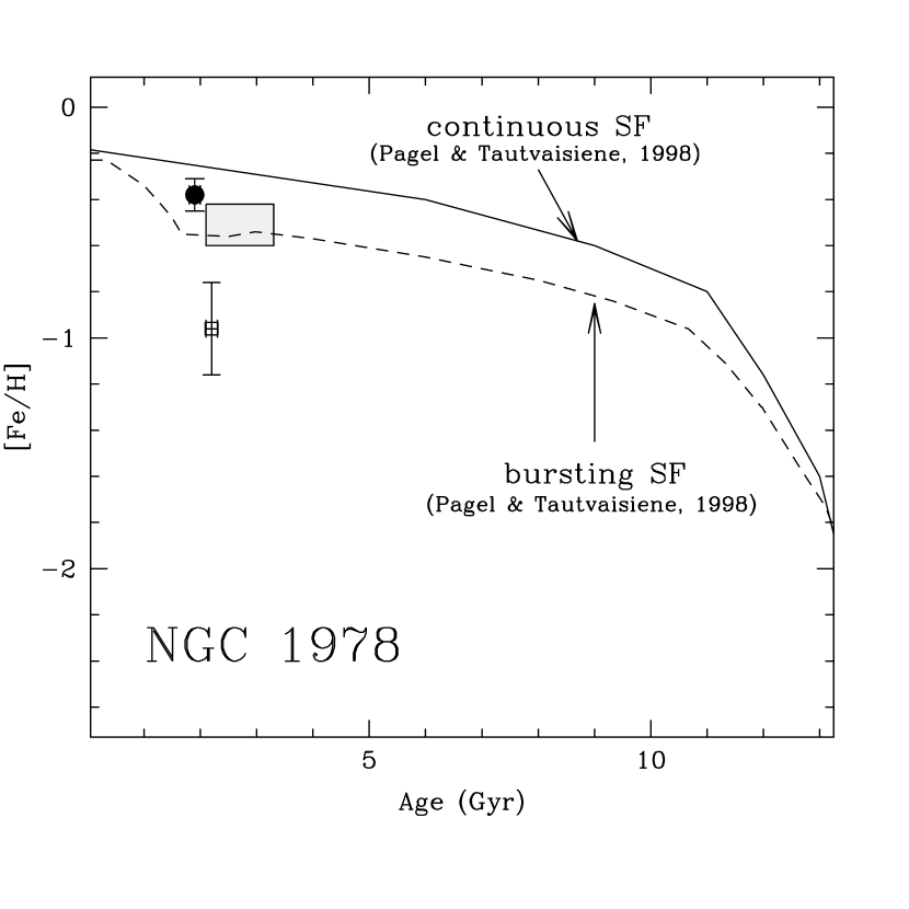
Figure 8: Theoretical predictions for the LMC AMR computed by Pagel & Tautvaisiene (1998): continuos line refers to a AMR obtained assuming a continuous SF, and dashed line corresponding to a bursting model. The black point indicates the position of NGC 1978 using the metallicity from Ferraro et al. (2006) and the age derived in this study. The open square refers the position for this cluster using metallicity by Hill et al. (2000) and age by Bomans et al. (1995). The grey box shows previous metallicity ($\rm-0.6<[Fe/H]<-0.4$) and age (2-3.3 Gyr) estimates from low resolution data.

References

- Alcaino et al. (1999) Alcaino, G., Liller, W., Alvarado, F., Kravtsov, V., Ipatov, A., Samus, N., & Smirnov, O., 1999, A&AS, 135, 103
- Alongi et al. (1991) Alongi, M., Bertelli, G., Bressan, A., & Chiosi, C., 1991, ASPC, 13, 223
- Alves (2004) Alves, D. R., 2004, New Astronomy Review, 48, 659
- Bhatia et al. (1991) Bhatia, R. K., Read, M. A., Hatzidimitriou, D., & Tritton, S.,1991, A&A, 87, 335
- Bedin et al. (2005) Bedin, L. R., Cassisi, S., Castelli, F., Piotto, G., Anderson, J., Salaris, M., Momany, Y. & Pietrinferni, A., 2005, MNRAS, 357, 1048
- Bekki et al. (2004) Bekki, K.,Couch, W. J.,Beasley, M. A., Forbes, D. A., Chiba, M., & Da Costa, G. S., 2004, ApJ, 610, L93
- Bellazzini et al. (2001) Bellazzini, M., Ferraro, F. R., & Pancino, E., 2001, MNRAS, 327, L15
- Bellazzini et al. (2002) Bellazzini, M., Ferraro, R. R., Origlia, L., Cacciari, C., Pancino, E., Monaco, L., & Oliva, E., 2002, AJ, 124, 3222
- Bessel, Castelli & Plez (1998) Bessel, M. S., Castelli, F., & Plez, B., 1998, A&A, 333, 231
- Bomans et al. (1995) Bomans, D. J., Vallenari, A., & de Boer, K. S., 1995, A&A, 298, 427
- Bohm-Vitense (1958) Bohm-Vitense, E., 1958, ZA, 46, 108
- Brocato et al. (1989) Brocato, E., Buonanno, R., Castellani, V., & Walker, A. R., 1989,ApJS, 71, 25
- Brocato et al. (1996) Brocato, E., Castellani, V., Ferraro, F. R.,Piersimoni, A. M.,& Testa, V.,1996, MNRAS, 282, 614
- Brocato et al. (2001) Brocato, E., Di Carlo, E., & Menna, G., 2001, A&A, 374, 523
- Castellani et al. (2003) Castellani, V.,Degl’Innocenti, S., Marconi, M., Prada Moroni, P.G., Sestito, P., 2003, A&A, 404, 645
- Clementini et al. (2003) Clementini, G., Gratton, R., Bragaglia, A., Carretta, E., Di Fabrizio, L., & Maio, M., 2003, AJ, 125, 1309
- Corsi et al. (1994) Corsi, C.E., Buonanno, R., Fusi Pecci, F., Ferraro, F.R., Testa, V., & Greggio, L., 1994, MNRAS, 271, 385
- de Freitas Pacheco, Barbuy & Idiart (1998) de Freitas Pacheco,J. A., Barbuy, B. & Idiart, T., 1998, A&A, 332, 19
- Dirsch et al. (2000) Dirsch, B., Richtler, T., Gieren, W. P., & Hilker, M., 2000,A&A, 360, 160
- Elson & Fall (1985) Elson, R. A., & Fall, S. M. 1985, ApJ, 299, 211
- Elson & Fall (1988) Elson, R. A., & Fall, S. M. 1988, AJ, 96, 1383
- Ferraro et al. (1995) Ferraro, F.R., Fusi Pecci, F., Testa, V., Greggio, L., Corsi, C.E., Buonanno, R., Terndrup, D.M., & Zinnecker, H., 1995, MNRAS, 272, 391
- Ferraro et al. (1999) Ferraro, F. R., Messineo, M., Fusi Pecci, F., de Palo, M. A., Straniero, O., Chieffi, A., & Limongi, M., 1999, AJ, 118, 1738
- Ferraro et al. (2004) Ferraro, F. R., Origlia, L., Testa, V. & Maraston, C., 2004, ApJ, 608, 772
- Ferraro et al. (2006) Ferraro, F. R.,Mucciarelli, A., Carretta, E., & Origlia, L., 2006, ApJ, 645, L33
- Fischer et al. (1992) Fischer P., Welch, D. L., & Mateo, M., 1992, AJ, 104, 3
- Fukunaga (1972) Fukunaga, K., 1972, ”Introduction to statististical pattern recognition”, Academic Press, New York
- Fusi Pecci et al. (1990) Fusi Pecci, F., Ferraro, F. R., Crocker, D. A., Rood, R. T., & Buonanno, R., 1990, A&A, 238, 95
- Geisler & Hodge (1980) Geisler D., & Hodge, P., 1980, ApJ, 242, 73
- Geisler et al. (1997) Geisler, D., Bica, E., Dottori, H., Claria, J. J., Piatti, A. E., & Santos, J. F. C. Jr., 1997, AJ, 114, 1920
- Girardi et al. (1995) Girardi, L., Chiosi, C., Bertelli, G., & Bressan, A. 1995, A&A, 298, 87
- Girardi et al. (2000) Girardi, L., Bressan, A., Bertelli, G. & Chiosi, C., 2000, A&AS, 141, 371
- Goodwin (1997) Goodwin, S., 1997, MNRAS, 186L, 39
- Hill et al. (2000) Hill, V., Francois, P., Spite, M., Primas, F., & Spite, F., 2000, A&AS, 364, 19
- Iben (1968) Iben, I., Jr., 1968, Nature, 220, 143
- King et al. (1984) King, C. R., Da Costa, G., & Demarque, P., 1984, ApJ, 299, 674
- Johnson et al. (2006) Johnson, J. A., Ivans, I. I.& Stetson, P. B., 2006, ApJ, 640, 801
- Kroupa (2001) Kroupa, P., 2001, MNRAS, 322, 231
- Larsen et al. (2000) Larsen, S. S., Clausen, J. V., & Storm, J., 2000, A&A, 364, 466
- Mackey & Gilmore (2003) Mackey, A. D. & Gilmore, G. F., 2004, MNRAS, 338, 85
- Mackey & Gilmore (2004) Mackey, A. D. & Gilmore, G. F., 2004, MNRAS, 352, 153
- Mackey et al. (2006) Mackey, A. D., Payne, M. J., & Gilmore, G. F., 2006, MNRAS,
- Mateo (1988) Mateo, M., 1988, ApJ, 331, 261
- Monaco et al. (2002) Monaco, L., Ferraro, F. R., Bellazzini, M., & Pancino, E., 2002, ApJ, 578. L50
- Mucciarelli et al. (2006) Mucciarelli, A., Origlia, L., Ferraro, F. R., Maraston, C., & Testa, V., 2006, ApJ, 646, 939
- Oliva & Origlia (1998) Oliva, E., & Origlia, L. 1998, A&A, 332, 46
- Olsen et al. (1998) Olsen, K. A. G., Hodge, P. W., Mateo, M., Olszewski, E. W., Schommer, R. A., Suntzeff, N. B., & Walker, A. R., MNRAS, 300, 665
- Olszewski (1984) Olszewski, E. W., 1984, ApJ, 284, 108
- Olszewski et al. (1991) Olszewski, E. W., Schommer, R. A., Suntzeff, N. B. & Harris, H. C., 1991, AJ, 101, 515
- Olszewski, Suntzeff & Mateo (1996) Olszewski, E.W., Suntzeff, N.B., & Mateo, M., 1996, ARA&A, 34, 511
- Origlia & Leitherer (2000) Origlia, L., & Leitherer, C., 2000, AJ, 119, 2018
- Pagel & Tautvaisiene (1998) Pagel, B. E. J., & Tautvaisiene, G., 1998, MNRAS, 299, 535
- Pancino et al. (2003) Pancino, E.,Seleznev, A., Ferraro, F. R., Bellazzini, M. & Piotto, G., 2003, MNRAS, 345, 690
- Persson et al. (1983) Persson, S. E., Aaronson, M., Cohen, J. G., Frogel, J. A., & Matthews, K.,1983, ApJ, 266, 105
- Pietrinferni et al. (2004) Pietrinferni, A., Cassisi, S., Salaris, M., & Castelli, F., 2004, ApJ, 612, 168
- Rich et al. (2001) Rich, M. R., Shara, M. M., & Zurek, D., 2001, AJ, 122, 842
- Salaris et al. (1993) Salaris, M., Chieffi, A., & Straniero, O., 1993, ApJ, 414, 580
- Salaris & Cassisi (2006) Salaris, M. & Cassisi, S., ”Evolution of stars and Stellar Populations”, Wiley, 2006
- Salpeter (1955) Salpeter, E. E., ApJ, 121, 161
- Scalo (1986) Scalo, J. M., 1986, Fundam. Cosmic. Phys., 11, 1
- Searle, Wilkinson, & Bagnuolo (1980) Searle, L., Wilkinson, A., & Bagnuolo, W. G. 1980, ApJ, 239, 803
- Sirianni et al. (2005) Sirianni M., et al., 2005, PASP, 117, 1049
- Stetson (1987) Stetson, P. B., 1987, PASP, 99, 191
- Straniero & Chieffi (1991) Straniero, O. & Chieffi, A., 1991, ApJS, 76, 525
- Testa et al. (1995) Testa, V., Ferraro, F. R., Brocato, V., & Castellani, V., 1995, MNRAS, 275, 454.
- Vallenari et al. (1994) Vallenari, A., Aparicio, A., Fagotto, F., & Chiosi, C., 1994, AJ, 284, 424
- van den Bergh (1981) van den Bergh, S., 1981, A&AS, 46, 79
- van den Bergh (1998) van den Bergh, S., 1998,PASP, 110, 1377
- Zoccali et al. (1999) Zoccali, M., Cassisi, S., Piotto, G., Bono, G., & Salaris, M., 1999, ApJ, 518, L49
- White & Shawl (1987) White, R.E., & Shawl, S. J., 1987, ApJ, 317, 246