Tiny-Scale Atomic Structure and the Cold Neutral Medium—Review and Recap

Abstract

Almost a decade ago I wrote an article with the same title as this. It focused on the physical properties of the Tiny-Scale Atomic Structure (TSAS) as discrete structures of the Cold Neutral Medium (CNM). To be observable, tiny discrete structures that don’t grossly violate pressure equilibrium need two attributes: low temperatures and geometrical anisotropy. Here I update that article. I discuss thermal and pressure equilibrium, ionization, optical lines, H₂ abundance, and evaporation.

Astronomy Department, University of California, Berkeley CA

1. Canonical Values for TSAS as Discrete Structures

Following Heiles (1997; H97), we use currently-available observations of the tiny-scale atomic structure (TSAS) to describe its properties; the observations have improved, so the inferred properties are now somewhat different. The TSAS is seen in 21-cm line absorption so must be part of the Cold Neutral Medium (CNM). The observations consist of time-variable 21-cm absorption lines against pulsars, VLBI images of the 21-cm line in absorption against extended radio sources, and optical absorption line observations against background stars. The canonical values for important properties come directly from these observations and have no theoretical or otherwise imaginary input, except for the subjective judgment and weighting that we must perform to collapse a variety of measured values into a single number that we can use as a canonical value. We provide values for the following properties:

1. TSAS column density:

   $$N(HI)_{TSAS,18}=0.75\,T_{15}\ ,$$ (1)

   where $N(HI)_{18}$ is the HI column density in units of $10^{18}$ cm^-2 and $T_{15}$ the temperature in units of 15 Kelvins (§3.1. justifies this canonical value of 15 K). The $T$-dependence arises because the 21-cm line opacity $\propto{1\over T}$. The numerical value 0.75 is 4 times larger than the canonical value adopted by H97 and is based on Weisberg & Stanimirovic (this meeting).

2. The TSAS scale length in the plane of the sky (denoted by the subscript $\perp$):

   $$L_{TSAS,\perp}=30\ {\rm AU}\ .$$ (2)

   The $\perp$ arises because with time variability and angular structure, it’s the plane-of-the-sky length that’s relevant.

3. The line-of-sight scale length $L_{TSAS,||}$ can be different (by a factor $G$) because it is unlikely for the structures to be isotropic:

   $$G\equiv{L_{TSAS,||}\over L_{TSAS,\perp}}\ .$$ (3)

4. We combine $N(HI)_{TSAS}$ and $L_{TSAS,||}$ to obtain the typical TSAS volume density:

   $$n(HI)_{TSAS}\equiv{N(HI)_{TSAS}\over L_{TSAS,||}}=1700\ {T_{15}\over G}\ {\rm cm^{-3}}\ .$$ (4)

5. The canonical values for volume density and temperature lead to the pressure $\widetilde{P}\equiv{P\over k}=nT$:

   $$\widetilde{P}_{TSAS}=26000\ {T_{15}^{2}\over G}\ .$$ (5)

With the above we make a simple, highly important observation: equation 5 shows that unless the TSAS is cold and/or anisotropic, its pressure greatly exceeds not only the typical CNM thermal pressure of $\widetilde{P}_{CNM}\sim 4000$ cm^-3 K, but also the Galactic hydrostatic pressure of $\widetilde{P}_{4K}\sim 28000$ cm^-3 K (Boulares & Cox 1990). This single point dominates the rest of the discussion, which includes some theoretical considerations.

2. Thermal Equilibrium, Thermal Pressure, and Total Pressure

Is the TSAS in thermal equilibrium? We normally expect the CNM to attain thermal equilibrium because the time scale is short. We have (Wolfire et al. 2003; WMHT)

$$t_{cool}={5\over 2}\ {1.1\ nkT\over n^{2}\Lambda}\ ,$$ (6)

where the symbols have their usual meanings and $n^{2}\Lambda$ is the cooling rate per cm^-3; cooling varies as $n^{2}$ because it is a collisional process. For collisional excitation of CII (the 158 $\mu$m line) by H atoms at $T=15$ K, which is the likely temperature of the TSAS, we have

$$t_{cool}=1.6\times 10^{4}\ G\ 460^{\left({1\over T_{15}}-1\right)}\ {\rm yr}\ .$$ (7)

or

$$t_{cool}=1.0\times 10^{5}\ {T_{15}^{2}\over\widetilde{P}_{TSAS}/\widetilde{P}_{CNM}}\ 460^{\left({1\over T_{15}}-1\right)}\ {\rm yr}\ .$$ (8)

Here $\widetilde{P}_{CNM}=4000$ cm^-3 K, our adopted pressure for the CNM. If the TSAS has ${T_{15}^{2}\over\widetilde{P}_{TSAS}/\widetilde{P}_{CNM}}\sim 1$, then $t_{cool}\sim 10^{5}$ yr. This is short by most interstellar standards. However, for the time- and space-variable TSAS it might not be short, so we consider two cases, the thermal equilibrium case and the nonequilibrium case.

2.1. Thermal Equilibrium Case

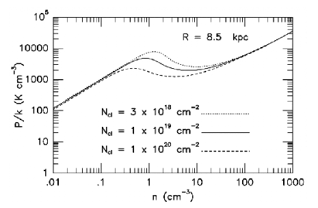
Figure 1.: The thermal-equilibrium pressure $\widehat{P}$ versus volume density $n(HI)$. Figure 9 from WMHT.

Suppose first that the TSAS is in thermal equilibrium. Then the density and pressure are related as shown in Figure 1, which is Figure 9 from WMHT. For discussion purposes, we use the solid curve for $N(HI)_{19}=1$ because we envision the TSAS to be embedded in CNM. At low and high $n(HI)$ it defines the Warm and Cold Neutral Media with temperatures $T\sim 8310$ and $\sim 62$ K, respectively.

The CNM thermal pressure has a minimum ($\widetilde{P}_{CNM,min}\sim 1960$ cm^-3 K) located near $n=10$ cm^-3. This minimum thermal pressure is defined by microscopic heating and cooling processes, which simply and unequivocally means that the CNM cannot exist in thermal equilibrium at lower thermal pressures. This is a strict lower limit for the CNM thermal pressure in thermal equilibrium. Similarly, the WNM has a microphysical-process thermal pressure maximum ($\widetilde{P}_{WNM,max}\sim 4810$ cm^-3 K) located near $n=1$ cm^-3.

There is no such strict microphysical-process upper limit on the CNM thermal pressure. However, there is an upper limit that arises from pressure-balance considerations. The CNM occupies a small fraction of the total interstellar volume, so it has to be embedded in warmer gas, either the WNM or the Hot Ionized Medium (HIM). If the interface is not dynamic it must have pressure balance. If the bounding medium is the WNM with no magnetic field, then the CNM thermal pressure must lie below $\widetilde{P}_{WNM,max}$; otherwise, the WNM is forbidden.

However, for dynamical equilibrium it’s the total pressure that counts, not just the thermal pressure. The WNM probably has the typical interstellar magnetic field of $\sim 6$ $\mu$G, which exerts a magnetic pressure of $\widetilde{P}_{mag}\lesssim 10^{4}$ cm^-3 K. This $\lesssim$ sign is important: it’s the magnetic pressure difference that counts, and even then only for that component that is perpendicular to the field lines, so if the field lines don’t lie along the interface, or if the CNM field is comparable to the WNM field, then the magnetic pressure difference is less. There’s a strict upper limit to the CNM pressure if it’s in thermal and dynamical equilibrium, which is the hydrostatic pressure of the Galactic disk; this is about $\widetilde{P}\sim 28000$ cm^-3 K (Boulares & Cox 1990). If there’s no magnetic field and no turbulence, then the CNM pressure has to lie in the very narrow range $\widetilde{P}\sim 1960$ to 4810 cm^-3 K, which is a factor of only 2.5.

In equation 5, for the strict upper limit $\widetilde{P}\sim 28000$ cm^-3 K, we require ${T_{15}^{2}\over G}\lesssim 1$. It’s unlikely, in our opinion, that the strict upper limit applies always. A more reasonable value is lower, perhaps $\widetilde{P}\sim 10000$ cm^-3 K, for which we require ${T_{15}^{2}\over G}\sim 0.4$. Below we will find that it is impossible to attain $T\lesssim 12$ K, so this implies $G\sim 2.5$. This seems like a perfectly reasonable degree of anisotropy for TSAS, particularly in light of H97’s estimate as $G\sim 10$ for a reasonable choice if TSAS is sheetlike.

2.2. Thermal Nonequilibrium Case

If we don’t have thermal equilibrium all bets are off and we can invoke any conditions we please. From the standpoint of making TSAS more easily explained by individual structures, we move toward smallness by invoking higher densities and pressures. For example, if $\widetilde{P}_{TSAS}=40000$ cm^-3 K, ten times higher than the equilibrium $\widetilde{P}_{CNM}$, $n_{TSAS}$ increases and $t_{cool}$ decreases by a factor of ten. The decreased cooling time presents the quandary that it’s harder to escape thermal equilibrium!

Raising the temperature above the lowest equilibrium value of 12 K is counterproductive in the sense of requiring higher HI column densities to produce observable 21-cm line absorption. Raising temperature instead of density also increases the cooling rate even more, because of the highly nonlinear factor $e^{-92{\rm K}\over T}$ in the cooling function $\Lambda$ (equation 9; for example, if we increase the temperature from 16 K to a typical CNM temperature of 60 K, the cooling rate $\Lambda$ would increase by a factor 100 (!).

Conclusion: if we invoke nonequilibrium, it’s easier to obtain the observed TSAS by keeping it cold and increasing the volume density. This, of course, also increases the pressure, which leads to some spectacular dynamics…

2.3. Dynamical Nonequilibrium Case

In the absence of pressure equilibrium, tiny-scale structures would expand rapidly into the surrounding medium. Soon the structures would no longer be “tiny”. For example, for a pressure ratio between TSAS and the surrounding medium of 10 the expansion velocity is close to Mach 10, or $\sim 0.3$ km s^-1; it takes only 500 years to expand by the TSAS characteristic scale size of 30 AU. So a structure won’t last long. On the other hand, one of the ways we detect TSAS is by time variability—which is a natural result of dynamical nonequilibrium! So, in this sense, dynamical nonequilibrium is suggested by the observations.

If the TSAS pressure is high, then you have to answer the question: how did the TSAS pressure get so high to begin with? The answer might be intermittency in the turbulence of the enveloping medium (Hily-Brandt, this meeting; Coles, this meeting).

To summarize: The nonequilibrium case has intrinsically high time variability. In this sense, it satisfies one of the observational signatures that define TSAS! This poses the question in a slightly different way: the observed time variability shows that TSAS is not in perfect dynamical equilibrium, but is it far from or not too far from equilibrium?

3. Physical Properties of the TSAS in Equilibrium

3.1. The Equilibrium Temperature

The equilibrium temperature is determined by equality of heating and cooling rates. Regarding cooling: The TSAS has no observed molecules, so we are left with the only effective atomic coolant, which is collisional excitation of CII. For cold gas, Carbon is almost fully ionized and Hydrogen almost fully neutral, so $n_{e}$ is almost equal to the gaseous Carbon abundance. We assume that the C/H abundance is $4\times 10^{-4}$ by number and that the gaseous C/H ratio is $\delta_{c}$ times smaller (some C goes into dust; people typically assume that the depletion factor $\delta_{c}=0.35$). We use WMHT equations C1 and C2 to write

$$n^{2}\Lambda=7.1\times 10^{-27}\delta_{c}\,n(HI)^{2}\ \left[T_{15}^{0.07}+\,0.41\,\delta_{c}\,T_{15}^{-0.5}\right]\,e^{-92/T}\ \rm{erg\ cm^{-3}\ s^{-1}}\ .$$ (9)

Note that there are two submechanisms: collisions by atomic HI (the first term) and by electrons (the second term). The H-collisions dominate, even there are no grains and $\delta_{c}=1$.

Heating is another matter. The commonly-accepted dominant heating mechanism is photoionization of PAH; this provides typical CNM temperatures of $\sim 60$ K. We envision TSAS temperatures to be much smaller, so we assume specifically that PAH heating (and, by implication, PAHs themselves) are absent. This has the ancillary consequence of freeing much of the Carbon to the gas phase, making $\delta_{c}\rightarrow 1$.

Without PAH heating, we have two possibly important heating mechanisms: photoionization of CI by starlight and ionization of HI by cosmic rays and soft X-rays. We first consider the former mechanism alone, which provides an absolute lower limit for the temperature of HI regions, and then include the latter.

Heating Exclusively by Photoionization of CI by Starlight

For heating by photoionization of CI, the heating rate per unit volume $n\Gamma$ is proportional to the photoionization rate per C atom multiplied by the volume density of C atoms $n(CI)$. In ionization equilibrium, the photoionization rate is equal to the recombination rate, and because Carbon is almost fully ionized the recombination rate is much easier to calculate. This gives

$$n\Gamma=\underbrace{n(CII)\,n_{e}\,\alpha(T)}_{\rm ioniz\ rate\ per\ cm^{-3}}\times\ \langle E_{i}\rangle\ ,$$ (10)

where $\alpha$ is the recombination coefficient. $E_{i}$ is the mean energy gained per photoionization; the UV radiation field drops to zero above 13.6 eV, so $E_{i}\approx(13.6\;{\rm eV}-I\!P_{C})/2$ (where $I\!P_{C}$ is Carbon’s ionization potential in eV; see Spitzer 1978, p. 107, p. 134-136, p. 142-143). Remembering that nearly all the electrons are contributed by gaseous Carbon, and that Carbon is almost fully ionized, we have

$$n\Gamma\approx 6.4\times 10^{-30}\delta_{c}^{2}\,n(HI)^{2}\,T_{15}^{-0.5}$$ (11)

We get the temperature by equating equations 9 and 11. If atomic H cooling (the first term in equation 9) is negligible, then (amazingly enough), as pointed out by Spitzer (1978, p. 143), we are left with the ultra-simple equation

$$e^{-92/T}=0.0022\ {\rm,\ or}$$ (12)

$$T=15.03\ {\rm K}\ .$$

This is a very robust result: it is independent of both the volume density (as long as $n(HI)\lesssim 3000$ cm^-3, where collisional de-excitation of CII becomes important) and the starlight intensity! Now, as we remarked above, H cooling does in fact dominate, which lowers the equilibrium temperature to about 12 K. This is a lower limit for the temperature in purely atomic regions.

The Heating Contribution from HI Ionization

The neural ISM has no UV photons above 13.6 eV energy, so HI can be ionized only by cosmic rays and soft X-rays. Soft X-rays are attenuated by small columns of HI, so their heating rate is sensitive to shielding. WMHT discuss this rather deeply and conclude that a typical primary ionization rate from soft X-rays is $\zeta_{X}\sim 1.6\times 10^{-17}$ s^-1 per H atom.

The primary ionization rate from cosmic rays $\zeta_{CR}$ is highly uncertain. For example, WMHT adopt $\zeta_{CR,WMHT}=1.8\times 10^{-17}$ sec^-1 per H-atom, a bit larger than $\zeta_{X}$. Three years later, Tielens (2005) adopts $\zeta_{CR,Tiel}=2\times 10^{-16}$ sec^-1 per H-atom, which is $11\,\zeta_{CR,WMHT}$! The difference is at least partly based on the measured abundance of the H${}_{3}^{+}$ ion (McCall et al 2002; Le Petit, Roueff, & Herbst 2004).

We have studied a cold ($T=17$ K) cloud that (surprisingly) lies within the Local Bubble (Meyer, this meeting and Meyer et al. 2006). I had hoped to be able to use the observed 17 K temperature of this cloud to establish an interesting upper limit on $\zeta_{CR}$ within the Local Bubble. However, the equilibrium temperature varies slowly with $\zeta_{CR}$: For $\delta_{c}=1$, $T$ rises to only 14.7 K for $\zeta_{CR}=\zeta_{CR,Tiel}$. Getting $T$ as high as 17 K requires $\zeta_{CR}\sim 6\zeta_{CR,Tiel}$. Evidently, the sensitivity of $T$ to $\zeta_{CR}$ is small! Just a little PAH heating could accomplish the same thing.

3.2. Optical Lines from Minority Ionization Species

Common optical interstellar absorption lines, like those of NaI, are produced by minority ionization species (ionization state $r$). If the next-higher ionization state ($r+1$) is the dominant one, then we have

$${n_{r}\over n_{r+1}}={\alpha n_{e}\over\Gamma}\ ,$$ (13)

where $\Gamma$ is the ionization rate of state $r$ and $\alpha$ is the recombination coefficient from $r+1$ to $r$. If these two ionization states comprise all of the element, then with $n_{r}\ll n_{r+1}$ the interstellar line strength (and $n_{r}$) $\propto\alpha n_{e}$. Typically $\alpha\propto T^{-0.6}$. If all the electrons come from Carbon, then $n_{e}\propto n(HI)\propto{P\over T}$. The total $T$ dependence is quite steep, $T^{-1.6}$—even steeper than for the 21-cm absorption line of HI [for which the absorption line strength $\propto N(HI)T^{-1}$].

Morton (1975) provides tables of $\Gamma$ and $\alpha_{56}$, where the subscript implies $\alpha$ evaluated at $T=56$ K. If one derives $n_{r}$ at 15 K instead of 56 K, the values are $\left(15\over 56\right)^{-0.6}=8.2$ times larger. More generally, with $n_{r}\ll n_{r+1}$ we have

$${n_{r}\over n_{tot}}\approx{\alpha_{56}\over\Gamma}\ 8.2\ {T_{15}^{1.62}\over\widetilde{P}_{TSAS}/\widetilde{P}_{CNM}}\ ,$$ (14)

where $n_{tot}$ is the volume density of both ionization states combined. For NaI and CI lines, ${\alpha_{56}\over\Gamma}=2.1$ and 11.7, respectively.

All of this implies that common absorption lines from minority ionization species in the TSAS should be strong.

3.3. H₂ Abundance

The H₂ molecule is formed on grains and destroyed by ultraviolet photons. The photon destruction occurs in spectral lines, which allows H₂ to shield itself; the destruction rate $\propto N(H_{2})^{-0.75}$. Tielens (2005) provides the numbers. For a flat slab illuminated on one side, the local volume density H₂ fraction is

$${n(H_{2})\over 2n(H)}=5\times 10^{-15}\ n(H)^{4}\ N(H)_{18}^{3}\ .$$ (15)

Here $n(H)$ is the total number of H-nuclei, including both H-atoms and H-molecules. Integrating in from the slab’s edge, the column density fraction is 4 times smaller.

Contrary to H97, the H₂ abundance is small; the difference comes from H97’s use of different numerical constants. This revision is favorable, because now H₂ doesn’t add to the TSAS pressure.

3.4. Environment: Evaporation

TSAS clouds are enveloped by a surrounding medium. This medium is another gas phase. Possible phases include warmer CNM, WNM, WIM, and HIM. The interface supports either evaporation of the embedded cloud to the environment, or condensation of the environment onto the embedded cloud.

Cowie & McKee (1977) provided the original treatment of the spherical cloud case. Jon Slavin’s talk at this meeting provides an excellent summary, including both the essential physics and convenient numerically-expressed equations; we use his equations in this paper. These processes are not intuitive, as our short discussion below illustrates. In particular, at the most basic level the mass loss rate depends only on $\kappa$, the thermal conductivity in the external medium, and the cloud radius $R_{c}$. For ionized external media, the effective conductivity $\kappa$ can be greatly reduced if magnetic field lines lie parallel to the boundary. Contrary to intuition, the mass loss rate per unit area is independent of cloud volume density $n_{cl}$. A very important concept is heat-flux saturation, which produces an upper limit on the evaporation rate.

For unsaturated evaporation, the most important and surprising point is that the mass loss rate per unit area of cloud is not independent of the radius of curvature $R_{c}$, but rather is proportional to $R_{c}^{-1}$; this results from the scaling of the gradient for spherical geometry. This means that, for a spherical cloud, the overall evaporation rate $\propto R_{c}$ instead of $R_{c}^{2}$ and the evaporation lifetime $\propto R_{c}^{2}$ instead of $R_{c}$. In contrast, the saturated evaporation rate per unit area $\propto R_{c}^{1/6}$ so the lifetime $\propto R^{7/6}$.

A second important concept is evaporation versus condensation: small clouds lose mass by evaporation, while large clouds gain mass by condensation. The critical radius $r_{crit}$ is given by Cowie & McKee Figure 2. For CNM embedded in WNM at $\widetilde{P}=4000$ cm^-3 K, $r_{crit}\sim 4000$ AU. If TSAS clouds are spherical, then they are smaller than this so they should evaporate. Similarly, TSAS should also evaporate when embedded in HIM.

But TSAS is almost certainly not spherical! The shapes of clouds really matter for evaporation. Thus, flat clouds, whose faces have infinite $R_{c}$, never evaporate but instead grow by condensation—on their faces. However, their edges can be sharp with small radii, where they can evaporate. Evaporation at the edges and condensation on the faces tends to push them towards sphericity.

TSAS evaporation is unsaturated when embedded in WNM and saturated in HIM. The evaporation timescale for spherical clouds having radius equal to the canonical $L_{\perp}=30$ AU of equation 2 is about 500 yr (this time $\propto R_{c}^{2}$) and 5000 yr (this time $\propto R_{c}^{7/6}$) in the WNM and HIM, respectively. These are short timescales, comparable to the dynamical timescale we estimated in §2.3. Both times are much shorter than times for thermal equilibrium.

There might not be a sharp interface. For example, TSAS clouds are probably very cold and have no grain heating. They might be surrounded by a thicker CNM envelope that contains grains, in which the temperature gradually increases outwards to perhaps 100 K or more; this would be an effective blanket against TSAS evaporation.

4. Summary

Section 1. provides canonical values for TSAS, assuming that it consists of discrete structures. Section 2. compares equilibrium versus nonequilibrium. In thermal equilibrium, with rough pressure equality the TSAS is so cold that the cooling rates are small; the thermal equilibrium time scale is $\sim 10^{5}$ yr, which might be too long for thermal equilibrium to be established. If the TSAS is not in thermal equilibrium, then it is probably warmer than 15 K, which exacerbates the TSAS overpressure problem and leads to dynamical nonequilibrium. If the TSAS is not in dynamical equilibrium, meaning that its internal pressure exceeds that of its surroundings, then the overpressure makes TSAS clouds expand, probably forcibly. TSAS exhibits time variability, which is not inconsistent with such expansion. However, if the TSAS is far from equilibrium, one must concoct a mechanism for its formation.

Section 3. discusses some physical processes in TSAS. TSAS is probably very cold, near the lower limit of $\sim 15$ K for optically thin molecule-free gas. Optical lines of minority species get stronger at low temperatures, and these lines should be strong in the TSAS. Evaporation and/or dynamical expansion limits TSAS lifetimes for spherical clouds, but maybe not for anisotropic clouds, magnetic fields, or unsharp cloud boundaries. Molecular hydrogen should not be plentiful in TSAS.

Acknowledgments.

It is a pleasure to thank Al Glassgold for helpful discussion. This research was supported in part by NSF grant AST-0406987.

References

- (1) Boulares, A. & Cox, D.P. 1990, ApJ, 365, 544
- (2) Cowie, L.L. & McKee, C.F. 1977, ApJ, 211, 135
- (3) Heiles, C. 1997, ApJ, 481, 193 (H97)
- (4) Le Petit, F., Roueff, E., & Herbst, E. 2004, A&A, 417, 993L
- (5) McCall, B.J., Hinkle, K.H., Geballe, T.R., Moriarty-Schieven, G.H., Evans, N.J., II, Kawaguchi, K., Takano, S., Smith, V.V., & Oka, T. 2002, ApJ, 567, 391
- (6) Meyer, D.M., Lauroesch, J.T., Heiles, C., Peek, J.E.G., & Engelhorn, K. 2006, ApJ, 650, L67
- (7) Morton, D.C. 1975, ApJ, 197, 85
- (8) Spitzer, L. Jr. 1978, Physical Processes in the Interstellar Medium (New York: Wiley), p. 143
- (9) Tielens, A.G.G.M. 2005, The Physics and Chemistry of the Interstellar Medium (Cambridge: Cambridge Univ Press)
- (10) Wolfire, M.G., McKee, C.F., Hollenbach, D., & Tielens, A.G.G.M. 2003, ApJ, 587, 278 (WMHT)