Density structure of the interstellar medium and the star formation rate in galactic disks

Abstract

The probability distribution functions (PDF) of density of the interstellar medium (ISM) in galactic disks and global star formation rate are discussed. Three-dimensional hydrodynamic simulations show that the PDFs in globally stable, inhomogeneous ISM in galactic disks are well fitted by a single log-normal function over a wide density range. The dispersion of the log-normal PDF (LN-PDF) is larger for more gas-rich systems, and whereas the characteristic density of LN-PDF, for which the volume fraction becomes the maximum, does not significantly depend on the initial conditions. Supposing the galactic ISM is characterized by the LN-PDF, we give a global star formation rate (SFR) as a function of average gas density, a critical local density for star formation, and star formation efficiency. Although the present model is more appropriate for massive and geometrically thin disks ($\sim 10$ pc) in inner galactic regions ($<$ a few kpc), we can make a comparison between our model and observations in terms of SFR, provided that the log-normal nature of the density field is also the case in the real galactic disk with a large scale height ($\sim 100$ pc). We find that the observed SFR is well-fitted by the theoretical SFR in a wide range of the global gas density ($10-10^{4}M_{\odot}$ pc^-2). Star formation efficiency (SFE) for high density gas ($n>10^{3}$ cm^-3) is SFE $=0.001-0.01$ for normal spiral galaxies, and SFE $=0.01-0.1$ for starburst galaxies. The LN-PDF and SFR proposed here could be applicable for modeling star formation on a kpc-scale in galaxies or numerical simulations of galaxy formation, in which the numerical resolution is not fine enough to describe the local star formation.

1. INTRODUCTION

The interstellar medium (ISM) in galaxies is characterized by highly inhomogeneous structure with a wide variety of physical and chemical states (Myers, 1978). Stars are formed in this complexity through gravitational instability in molecular cores, but the entire multi-phase structures on a global scale are quasi-stable. It is therefore important to understand theoretically the structure of the ISM in a wide dynamic range to model star formation in galaxies. Observations suggest that there is a positive correlation between global star formation rate (SFR) and the average gas density: $\dot{\Sigma}_{\star}\propto\Sigma_{gas}^{N}$ with $N\sim 1.4$ in nearby galaxies (Kennicutt, 1998). Since star formation process itself is a local phenomenon on a sub-parsec scale, the observed correlation between the structure of the ISM on a local scale and the global quantities, such as the average gas density, implies that the ISM on different scales is physically related.

In fact, two- and three-dimensional hydrodynamic and magneto-hydrodynamic simulations (e.g. Bania & Lyon, 1980; Vazquez-Semadeni, Gazol, & Scalo, 2000; Rosen & Bregman, 1995; de Avillez, 2000) show that there is a robust relation between the local and global structures of the multi-phase ISM, which is described by a log-normal density PDF (probability distribution function). Elmegreen (2002) first noticed that if the density PDF is log-normal and star formation occurs in dense gases above a critical density, the Schmidt-Kennicutt law is reproduced. This provides a new insight on the origin of the scaling relation. More recently Krumholz & McKee (2005) give a similar model on SFR in molecular clouds. In these theoretical predictions, dispersion of the LN-PDF, $\sigma$, is a key parameter. Elmegreen (2002) used $\sigma=2.4$, which is taken from 2-D hydrodynamic simulations of the ISM (Wada & Norman, 2001). Krumholz & McKee (2005) assumed an empirical relation between $\sigma$ and the rms Mach number, which is suggested in numerical simulations of isothermal turbulence (see also §4.1). Therefore, it is essential to know whether the LN-PDF in galactic dicks is universal, and what determines $\sigma$. However, most previous simulations, in which LN-PDF or power-law PDF are reported, are ‘local’ simulations: a patch of the galactic disk is simulated with a periodic boundary condition. Apparently, such local simulations are not suitable to discuss statistical nature of the ISM in galactic disks. For example, number of density condensations are not large enough (typically a few) (see Scalo et al., 1998; Slyz et al., 2005).

On the other hand, global hydrodynamic simulations for two-dimensional galactic disks or three-dimensional circum-nuclear gas disks suggested that the density PDF, especially a high-density part is well fitted by a single log-normal function over 4-5 decades (Wada & Norman 1999, 2001, hereafter WN01 and Wada 2001). The log-normal PDF is also seen in a high-z galaxy formed by a cosmological N-body/AMR(Adaptive Mesh Refinement) simulation (Kravtsov, 2003). Nevertheless universality of LN-PDF and how it is related to global quantities are still unclear.

In this paper, we verify the log-normal nature of the ISM in galactic disks, using three-dimensional, global hydrodynamic simulations. This is an extension of our previous two-dimensional studies of the ISM in galactic disks (WN01) and three-dimensional model in the galactic central region (Wada & Norman, 2002). We confirm that dispersion $\sigma$ of the log-normal function is related to average gas density of the disk. We then calculate SFR as a function of critical density of local star formation and star star formation efficiency. This is a generalized version of the Schmidt-law (Schmidt, 1959), and it can be applied to various situations.

An alternative way to study the global SFR in galaxies is simulating star formation directly in numerical models (e.g. Li, Mac Low, & Klessen, 2006; Kravtsov & Gnedin, 2005; Tasker & Bryan, 2006). In this approach, ‘stars’ are formed according to a ‘star formation recipe’, and the resultant SFR is compared to observations. We do not take this methodology, because numerical modeling star formation in simulations still requires many free-parameters and assumptions. Moreover if the numerically obtained SFR deviates from the observed scaling relation (this is usually the case. See for example Tasker & Bryan 2006), it is hard to say what we can learn from the results. This deviation might be due to wrong implementation of star formation in the numerical code, or estimate of SFR in observations might be wrong, since SFR is not directly observable. One should also realize that comparison with observations of local galaxies is not necessarily useful when we discuss SFR in different situations, such as galaxy formation. In this paper, we avoid the ambiguity in terms of star formation in simulations, and alternatively discuss SFR based on an intrinsic statistical feature of the ISM. Effect of energy feedback from supernovae is complementarily discussed.

This paper is organized as follows. In §2, we describe results of numerical simulations of the ISM in a galactic disk, focusing on the PDF. In §3, we start from a ‘working-hypothesis’, that is the inhomogeneous ISM, which is formed through non-linear development of density fluctuation, is characterized by a log-normal density PDF. After summarizing basic properties of the LN-PDF, we use the LN-PDF to estimate a global star formation rate, and it is compared with observations. In §4, we discuss implications of the results in §2 and §3. In order to distinguish local (i.e. sub-pc scale) and global (i.e. galactic scale) phenomena, we basically use cm^-3 for local number density and $M_{\odot}$ pc^-3 (or $M_{\odot}$ pc^-2) for global density.

2. GLOBAL SIMULATIONS OF THE ISM IN GALACTIC DISKS AND THE PDF

2.1. Numerical Methods

Evolution of rotationally supported gas disks in a fixed (i.e. time-independent), spherical galactic potential is investigated using three-dimensional hydrodynamic simulations. We take into account self-gravity of the gas, radiative cooling and heating processes. The numerical scheme is an Euler method with a uniform Cartesian grid, which is based-on the code described in WN01 and Wada (2001). Here we briefly summarize them. We solve the following conservation equations and Poisson equation in three dimensions.

$$\frac{\partial\rho}{\partial t}+\nabla\cdot(\rho\mbox{\boldmath${v}$}) = 0,$$ (1)

$$\frac{\partial\mbox{\boldmath${v}$}}{\partial t}+(\mbox{\boldmath${v}$}\cdot\nabla)\mbox{\boldmath${v}$}+\frac{\nabla p}{\rho}+\nabla\Phi_{\rm ext}+\nabla\Phi_{\rm sg} = 0,$$ (2)

$$\frac{\partial(\rho E)}{\partial t}+\nabla\cdot[(\rho E+p)\mbox{\boldmath${v}$}] = \rho\Gamma_{\rm UV}+\Gamma_{\rm SN}-\rho^{2}\Lambda(T_{g}),$$ (3)

$$\nabla^{2}\Phi_{\rm sg} = 4\pi G\rho,$$ (4)

where, $\rho,p,\mbox{\boldmath${v}$}$ are the density, pressure, velocity of the gas. The specific total energy $E\equiv|\mbox{\boldmath${v}$}|^{2}/2+p/(\gamma-1)\rho$, with $\gamma=5/3$. The spherical potential is $\Phi_{\rm ext}\equiv-(27/4)^{1/2}[v_{1}^{2}/(r^{2}+a_{1}^{2})^{1/2}+v_{2}^{2}/(r^{2}+a_{2}^{2})^{1/2}]$, where $a_{1}=0.3$ kpc, $a_{2}=5$ kpc, and $v_{1}=v_{2}=200$ km s^-1. We also assume a cooling function $\Lambda(T_{g})$ $(10<T_{g}<10^{8}{\rm K})$ (Spaans & Norman, 1997) with solar metallicity. We assume photo-electric heating by dust and a uniform UV radiation field, $\Gamma_{\rm UV}=1.0\times 10^{-23}\varepsilon G_{0}\,{\rm ergs\>s}^{-1},$ where the heating efficiency $\varepsilon$ is assumed to be 0.05 and $G_{0}$ is the incident FUV field normalized to the local interstellar value (Gerritsen & Icke, 1997). In order to focus on a intrinsic inhomogeneity in the ISM due to gravitational and thermal instability, first we do not include energy feedback from supernovae. In §4.5 we show a model with energy feedback from supernovae (i.e. $\Gamma_{\rm SN}\neq 0$). Note that even if there is no random energy input from supernovae, turbulent motion can be maintained in the multi-phase, inhomogeneous gas disk (Wada, Meurer, & Norman, 2002).

The hydrodynamic part of the basic equations is solved by AUSM (Advection Upstream Splitting Method) (Liou & Steffen, 1993) with a uniform Cartesian grid. We achieve third-order spatial accuracy with MUSCL (Monotone Upstream-centered Schemes for Conservation Laws) (van Leer, 1977). We use $512\times 512\times 64$ grid points covering a $2.56\times 2.56\times 0.32$ kpc³ region (i.e. the spatial resolution is 5 pc). For comparison, we also run models with a 10 pc resolution. The Poisson equation is solved to calculate self-gravity of the gas using the Fast Fourier Transform (FFT) and the convolution method (Hockney & Eastwood, 1981). In order to calculate the isolated gravitational potential of the gas, FFT is performed for a working region of $1024\times 1024\times 128$ grid points (see details in WN01). We adopt implicit time integration for the cooling term. We set the minimum temperature, for which the Jeans instability can be resolved with a grid size $\Delta$, namely $T_{\rm min}=35$ K ($\rho/10M_{\odot}$ pc${}^{-3})(\Delta/5\;{\rm pc})^{2}$.

The initial condition is an axisymmetric and rotationally supported thin disk (scale height is 10 pc) with a uniform density $\rho_{i}$. We run four models with different $\rho_{i}$ (see Table 1). Random density and temperature fluctuations are added to the initial disk. These fluctuations are less than 1 % of the unperturbed values and have an approximately white noise distribution. The initial temperature is set to $10^{4}$ K over the whole region. At the boundaries, all physical quantities remain at their initial values during the calculations.

Table 1Initial density and fitting parameters of the density PDF

Model	$\rho_{i}$   ($M_{\odot}$ pc-3)	$\sigma_{10}$	$\sigma$	$\log\rho_{0}$	$\alpha$	$\sigma_{10,M}$	$\sigma_{M}$	$\sigma_{p}$
A	5	1.025	2.360	-1.40	0.09	1.025	2.360	2.483
B	10	1.188	2.735	-1.55	0.12	1.188	2.735	2.769
C	15	1.223	2.816	-1.60	0.18	1.273	2.849	2.810
D	50	1.308	3.012	-1.50	0.20	1.308	3.012	3.104

2.2. Numerical Results

Figure 1 is snapshots of density distribution at a quasi-stable state for models A, B and D on the x-y plane and x-z plane. Depending on the initial density ($\rho_{i}=5,10$, and 50 $M_{\odot}$ pc^-3), distribution of the gas in a quasi-equilibrium is different. In the most massive disk (Fig. 1c, model D), the disk is fragmented into clumps and filaments, on the other hand, the less massive disk (Fig. 1a, model A) shows more axi-symmetric distribution with tightly winding spirals and filaments. In Fig. 2, we show vertical structures of density of model D ($t=42$ Myr). The high density disk ($\rho>0.1M_{\odot}$ pc^-3) is resolved by about 10 grid points out of 64 total grid points for $z$-direction. Density change in about 5 orders of magnitude from the disk to halo gas is resolved.

Figure 3 is time evolution of a density PDF in model D. The initial uniform density distribution, which forms the peak around $\rho\simeq 50M_{\odot}$ pc^-3, is smoothed out in $\sim 10$ Myr, and it turns out to a smooth distribution in $\sim 20$ Myr. Figure 4 is PDFs spatially de-convolved to four components (thin disk, thick disk in the inner disk, halo, and the whole computational box. See figure caption for definitions) of model D in a quasi-steady state ($t=32$ Myr). It is clear that dense regions ($\rho\gtrsim 0.01M_{\odot}$ pc^-3) can be fitted by a single log-normal function, $f_{\rm LN}$, over nearly 6 decades:

$$f_{\rm LN}(\rho;\rho_{0},\sigma_{10})=\frac{\alpha}{\sqrt{2\pi}\sigma_{10}\ln 10}\exp{\left[-\frac{\log(\rho/\rho_{0})^{2}}{2\sigma_{10}^{2}}\right]},$$ (5)

where $\alpha$ is volume fraction of the high-density part which is fitted by the LN-PDF. On a galactic scale, the ISM is a multi-phase, and dense, cold gases occupy smaller volumes than diffuse, hot gases. Therefore, it is reasonable that the density PDF shows a negative slope against density as shown in the previous numerical simulations. However, our results suggest that structure of the ISM is not scale-free. The LN-PDF implies that formation process for the high density part is highly non-linear (Vazquez-Semadeni, 1994). High density regions can be formed by convergent processes, such as mergers or collisions between clumps/filaments, compressions by sound waves or shock waves. Tidal interaction between clumps and galactic shear or local turbulent motion can also change their density structure. For a large enough volume, and for a long enough period, these processes can be regarded as many random, independent processes in a galactic disk. In this situation, the density in a small volume is determined by a large number of independent random events, which can be expressed by $\rho=\Pi_{i=1}^{i=N}\delta_{i}\rho_{s}$ with independent random factors $\delta_{i}$ and initial density $\rho_{s}$. Therefore the distribution function of $\log(\rho)$ should be Gaussian according to the central limit theorem, if $N\rightarrow\infty$.

In Table 1, we summarize fitting results for the PDF in the four models in terms of the whole volume. One of important results is that there is a clear trend that the dispersion is larger for more massive systems. The less massive model (model B) also shows a LN-PDF (Fig. 5), but the dispersion is smaller ($\sigma_{10}=1.188$) than that in model D. The PDF for the whole volume is log-normal, but there is a peak around $\log\rho=1.3$. As shown by the dotted line, this peak comes from the gas just above the disk plane ($10\leq z\leq 20$ pc) in the inner disk ($r\lesssim 0.38$ kpc), where the gas is dynamically stable, and therefore the density is not very different from its initial value ($\rho_{i}=10$). This peak is not seen in the dotted line in model D (Fig. 4), since the density field in model D is not uniform even in the inner region due to the high initial density.

The excess of the volume at low density ($\lesssim 10^{-3}M_{\odot}$ pc^-3, see Figs. 4 and 5) is due to a smooth component that is extened vertically outside the thin, dense disk. About 10-20% of the whole computational box is in the LN regime (i.e. $\alpha=0.1-0.2$). However, most fraction of mass is in the LN regime (see Fig. 9).

In order to ensure that gravitational instability in high density gas is resolved, we set the minimum temperature $T_{\rm min}$, depending on a grid-size (§2.1). We run model C with two different resolutions, 5 pc and 10 pc. As seen in Fig. 6, although the “tangled web” structure is qualitatively similar between the two models, typical scales of the inhomogeneity, e.g. width of the filaments, are different. The scale height of the disk $H$ in the model with $\Delta=5$ pc is about a factor of two smaller than the model with $\Delta=10$ pc. This is reasonable, since $T_{\rm min}\propto\Delta^{2}$ and $H\propto T_{g}^{1/2}$,if the disk is vertically in a hydrostatic equilibrium. In Fig. 7, we compare density PDF in the two models with different spatial resolution. PDFs in the models are qualitatively similar, in a sense that the PDF has a LN part for high density gas, although the PDF in the model with a 10 pc resolution is not perfectly fitted by a LN function. This comparison implies that the spatial resolution should be at least 5 pc in order to discuss PDF of the ISM in galactic disks.

Figure 8 shows a phase-diagram of model D. Two dominant phases in volume, i.e. warm gas $T_{g}\sim 8000$ K and cold gas ($T_{g}\sim 30-1000$K) exist. Temperature of the gas denser than $\rho\simeq 10M_{\odot}$ pc^-3 is limitted by $T_{\rm min}$. As suggested by Fig. 8, frequency distribution of temperature is not represented by a single smooth function, which is a notable difference to density PDF. High density gas ($\rho>10^{-2}M_{\odot}$ pc^-3) is not isothermal, suggesting that isothermality is not a necessary condition for the LN density PDF in global models of the ISM (see also §4.1).

As qualitatively seen in Fig. 1, the dispersion of LN-PDF is larger in more massive system. This is more quantitatively seen in Fig. 9, mass-weighted PDFs in 4 models with different $\rho_{i}$. In the fit, we use the same $\sigma$ obtained from the volume-weighted PDF, and the mass-weighted characteristic density $\rho_{0,M}$ is calculated using

$$\rho_{0,M}=\rho_{0}e^{\sigma^{2}}.$$ (6)

Equation (6) is always true if the PDF is log-normal. The dispersion $\sigma$ is 2.36 in model A ($\rho_{i}=5M_{\odot}$ pc^-3) and 3.01 in model D ($\rho_{i}=50M_{\odot}$ pc^-3) (Table 1). The dependence of $\sigma$ on the initial gas density (or total gas mass) is a natural consequence of LN-PDF (see §3.1). From comparison between the volume-weighted and mass-weighted PDF, it is clear that even if the smooth non-LN regime occupy the most part of the volume of the galactic disk-halo region (i.e. $\alpha<1$), the mass of ISM is dominated by the LN-PDF regime.

Another important point in the numerical results is that the characteristic density of LN-PDF, $\rho_{0}$, does not significantly change among the models, despite the wide (almost 8 orders of magnitude) density range in the quasi-steady state. In fact, as shown in Table 1, $\rho_{0}$ is in a range of $1.7<\rho_{0}<2.7$ cm^-3 among the models with $\rho_{i}=5-50M_{\odot}$ pc^-3. Physical origin of this feature is discussed in §3.1.

In summary, using our three-dimensional high resolution hydrodynamic simulations, we find that the ISM in a galactic disk is inhomogeneous on a local scale, and it is consisted of many filaments, clumps, and low-density voids, which are in a quasi-steady state on a global scale. Statistical structure of the density field in the galactic disks is well described by a single LN-PDF over 6 decades in a high density part (i.e. $\rho\gtrsim 0.01M_{\odot}$ pc^-3). Most part of the mass is in the regime of LN-PDF. The dispersion of the LN-PDF is larger for more massive system.

3. PROBABILITY DISTRIBUTION FUNCTION AND THE STAR FORMATION RATE

3.1. Basic Properties of the Log-Normal PDF

In this section, based on properties of LN-PDF, we discuss how we can understand the numerical results in §2. Suppose that the density PDF, $f(\rho)$ in the galactic disk is described by a single log-normal function:

$$f(\rho)d\rho=\frac{1}{\sqrt{2\pi}\sigma}\exp{\left[-\frac{\ln(\rho/\rho_{0})^{2}}{2\sigma^{2}}\right]}d\ln\rho,$$ (7)

where $\rho_{0}$ is the characteristic density and $\sigma$ is the dispersion. The volume average density $\langle\rho\rangle_{V}$ for the gas described by a the LN-PDF is then

$$\langle\rho\rangle_{V} = \frac{1}{\sqrt{2\pi}\sigma}\int^{\infty}_{-\infty}\rho\exp{\left[-\frac{\ln(\rho/\rho_{0})^{2}}{2\sigma^{2}}\right]}d\ln\rho,$$ (8)

$$= \rho_{0}\,e^{{\sigma^{2}}/{2}}.$$ (9)

The mass-average density is

$$\langle\rho\rangle_{M} \equiv \frac{\int\rho^{2}dV}{M_{t}}=\rho_{0,M}e^{\sigma^{2}}=\rho_{0}e^{2\sigma^{2}}$$ (10)

where $M_{t}=\int\rho dV$ is the total mass in the log-normal regime. The dispersion $\sigma$ of the LN-PDF is therefore

$$\sigma^{2}=\frac{2}{3}\ln\left(\frac{\langle\rho\rangle_{M}}{\langle\rho\rangle_{V}}\right).$$ (11)

Equivalently, using $\rho_{0}$,

$$\sigma^{2} = 2\ln\left(\frac{\langle\rho\rangle_{V}}{\rho_{0}}\right)$$ (12)

$$= \frac{1}{2}\ln\left(\frac{\langle\rho\rangle_{M}}{\rho_{0}}\right).$$ (13)

Suppose the characteristic density $\rho_{0}$ is nearly constant as suggested by the numerical results, Equations (12) or (13) tells that the dispersion $\sigma$ is larger for more massive systems, which is also consistent with the numerical results. For a stable, uniform system, i.e. $\langle{\rho}\rangle_{V}=\rho_{0}$, $\sigma$ should be zero. In another extreme case, namely $\langle{\rho}\rangle_{V}\rightarrow\infty$, $\sigma\rightarrow\infty$, but this is not the case, because the system itself is no longer dynamically stable. Therefore, $\sigma$ should take a number in an appropriate range in a globally stable, inhomogeneous systems. Galactic disks are typical examples of such systems.

In our numerical results, the ISM with low density part (typically less than $10^{-3}M_{\odot}$ pc^-3) is not fitted by the LN-PDF. If density field of the ISM in a fraction, $\alpha$, of the arbitrarily volume is characterized by the LN-PDF, the volume average density in the volume is $\bar{\rho}=\alpha\langle\rho\rangle_{V}$. In this case, eq. (12) is modified to

$$\sigma_{p}^{2}=2\ln\left(\frac{\bar{\rho}}{\alpha\rho_{0}}\right).$$ (14)

As shown in Table 1, $\sigma$ in the numerical results well agrees with $\sigma_{p}$ in each model. In numerical simulations, it is easy to know the volume in the LN-regime (i.e. $\alpha\times$ volume of the computational box), therefore calculating $\sigma_{p}$ is straightforward using eq. (14). However, if one wants to evaluate $\sigma$ from observations of galaxies, it is more practical to use the mass-average density, eq. (13), because it is expected that mass of the galactic ISM is dominated by the LN-regime in mass (see Fig. 9).

Interestingly, even if the density contrast is extremely large (e.g. $10^{6}-10^{8}$), the numerical results show that the characteristic density $\rho_{0}$ is not sensitive for the total gas mass in a kpc galactic disk ($\rho_{0}=1.7-2.7$ cm^-3). If this is the case, what determines $\rho_{0}$? In Fig. 10, we plot effective pressure, $p_{\rm eff}\equiv p_{\rm th}+\rho v_{t}^{2}$ as a function of density, where $p_{\rm th}$ is the thermal pressure, and $v_{t}$ is turbulent velocity dispersion, which is obtained by averaging the velocity field in each sub-region with a (10 pc)³ volume. If the turbulent motion in a volume with a size $L$ is originated in selfgravity of the gas and galactic rotation(Wada, Meurer, & Norman, 2002), $p_{\rm eff}\sim\rho GM_{g}/L\propto\rho^{4/3}$, provided that the mass in the volume $M_{g}$ is conserved (i.e. $\rho\propto L^{-3}$). In fact, Fig. 10 shows that a majority of the gas in the dense part ($\rho\gtrsim 10^{-1}M_{\odot}$ pc^-3) follows $p_{\rm eff}\propto\rho^{4/3}$. On the other hand, for the low density regime, $p_{\rm eff}\propto\rho^{2/3}$. In the present model, a dominant heating source in low density gases is shock heating. Shocks are ubiquitously generated by turbulent motion, whose velocity is $\sim$ several 10 km s^-1. The kinetic energy is thermalized at shocks, then temperature of low density gas goes to $T_{g}\sim 10^{4-5}$ K. In supersonic, compressible turbulence, its energy spectrum is expected to be $E(k)\propto k^{-2}$, where total kinetic energy $E_{t}=\int E(k)dk$. Therefore $p_{\rm eff}\propto\rho v^{2}\propto\rho^{2/3}$, because $v^{2}\propto k^{-1}\propto\rho^{-1/3}$. Then the ‘effective’ sound velocity $c_{\rm eff}^{2}\equiv dp_{\rm eff}/d\rho\propto\rho^{-1/3}$ and $c_{\rm eff}^{2}\propto\rho^{1/3}$ for the low and high density regions, respectively. This means that the effective sound velocity $c_{\rm eff}$ has a minimum at the transition density ($\rho_{t}$) between the two regimes. In other words, since $c_{\rm eff}^{2}=c_{s}^{2}+v_{t}^{2}$, there is a characteristic density below/above which thermal pressure/turbulent pressure dominates the total pressure, i.e. $c_{s}^{2}\sim v_{t}^{2}$. Thus,

$$\frac{kT_{g}}{\mu}\sim\frac{GM_{g}}{L}\sim G\rho_{t}L^{2},$$ (15)

where $\mu$ is average mass per particle, and $L$ is size of the largest eddy of gravity-driven turbulence, which is roughly the scale height of the disk. As seen in Fig. 8, gas temperature around $\rho_{0}=10^{-1.5}M_{\odot}$ pc^-3 is $T_{g}\sim 80$ K. The scale height of the dense disk is about 10 pc (Fig. 2) in the present model, therefore

$$\rho_{t}\simeq 1\;\;\;{\rm cm}^{-3}\left(\frac{T_{g}}{80\;{\rm K}}\right)\left(\frac{L}{10\;{\rm pc}}\right)^{-2}.$$ (16)

This transition density is close to the characteristic density in the numerical results, i.e. $\rho_{0}=10^{-1.4}-10^{-1.6}M_{\odot}$ pc^-3($\approx$ 2.7 - 1.7 cm^-3). In a high-density region ($\rho>\rho_{t}\approx\rho_{0}$), stochastic nature of the system, which is the origin of the log-normality, is caused in the gravity-driven turbulence, and for low density regions its density field is randomized by thermal motion in hot gases. For the gases around $\rho_{0}$, the random motion is relatively static, therefore probability of the density change is small. As a result, the density PDF takes the maximum around $\rho_{0}$. An analogy of this phenomenon is a snow or sand drift in a turbulent air. The material in a turbulent flow is stagnated in a relatively “static” region.

As seen in Fig. 2, the present gas disk has a much smaller scale height than the ISM in real galaxies, which is about 100 pc. If turbulent motion in galactic disks is mainly caused by gravitational and thermal instabilities in a rotating disk (Wada, Meurer, & Norman, 2002), we can estimate $\rho_{t}$ by eq. (16) in galactic disks, but gas temperature of the dominant phase in volume is $T_{g}\sim 10^{4}$ K, as suggested by two-dimensional models (Wada & Norman, 2001). Therefore, we expect that $\rho_{t}\sim 1$ cm^-3 is also the case in real galaxies. However, if the turbulent motion in ISM is caused by different mechanisms, such as supernova explosions, magneto-rotational instabilities, etc., dependence of $p_{\rm eff}$ on density could be different from $p_{\rm eff}\propto\rho^{4/3}$, and as a result $\rho_{t}\sim$ const. $\sim O(1)$ cm^-3 could not be always true. Determining $\rho_{0}$ in a much larger disk than the present model, taking into account various physics is an important problem for 3-D simulations with a large dynamic range in the near future. In §3.3, we compare our results with SFR in spiral and starburst galaxies, in which $\rho_{0}$ is treated as one of free parameters (see Fig. 12 and related discussion).

Suppose the volume average density is $\langle\rho\rangle_{V}=3M_{\odot}$ pc^-3, we can estimate the dispersion $\sigma$ is $\sigma\simeq 3$ for $\rho_{0}=1$ cm^-3 from eq. (12). For a less massive system, e.g. $\langle\rho\rangle_{V}=0.3M_{\odot}$ pc^-3, $\sigma\simeq 2.1$. Therefore we can expect a larger star formation rate for more massive system, since a fraction of high density gas is larger. Using this dependence of $\sigma$ on the average gas density, we evaluate global star formation rate in the next section.

3.2. Global Star Formation Rate

Based on the numerical results in §2 and the properties of LN-PDF described in §3.1, we here propose a simple theoretical model of the star formation on a global scale. We assume that the multi-phase, inhomogeneous ISM in a galactic disk, can be represented by a LN-PDF. Elmegreen (2002) discussed a fraction of high density gas and global star formation rate assuming a LN-PDF. Here we follow his argument more specifically.

If star formation is led by gravitational collapse of high-density clumps with density $\rho_{c}$, the star formation rate per unit volume, $\dot{\rho_{\star}}$, can be written as

$$\dot{\rho_{\star}}=\epsilon_{c}(G\rho_{c})^{1/2}f_{c}\langle\rho\rangle_{V}$$ (17)

where $f_{c}(\rho_{c},\sigma)$ is a mass fraction of the gas whose density is higher than a critical density for star formation ($\rho>\rho_{c}$), and $\epsilon_{c}$ is the efficiency of the star formation.

Suppose the ISM model found in §2, whose density field is characterized by LN-PDF, is applicable to the ISM in galactic disk, $f_{c}$ is

$$f_{c}(\delta_{c},\sigma) = \frac{\int^{\infty}_{\ln\delta_{c}}\delta\exp\left[-\frac{(\ln\delta)^{2}}{2\sigma^{2}}\right]d(\ln\delta)}{\int^{\infty}_{-\infty}\delta\exp\left[-\frac{(\ln\delta)^{2}}{2\sigma^{2}}\right]d(\ln\delta)},$$ (18)

$$= \frac{1}{2}(1-{\rm Erf}[z(\delta_{c},\sigma)])\;,$$ (19)

where $\delta\equiv\rho/\rho_{0}$, $\delta_{c}\equiv\rho_{c}/\rho_{0}$, and

$$z(\delta_{c},\sigma)\equiv\frac{\ln\delta_{c}-\sigma^{2}}{\sqrt{2}\sigma}.$$ (20)

The fraction of dense gas, $f_{c}$ is a monotonic function of $\delta_{c}$ and $\sigma$, and it decreases rapidly for decreasing $\sigma$. Suppose $\delta_{c}=10^{5}$, $f_{c}\sim 10^{-2}$ for $\sigma=3.0$, and $f_{c}\sim 10^{-6}$ for $\sigma=2.0$. The star formation rate (eq. (17)) per unit volume then can be rewrite as a function of $\epsilon_{c},\delta_{c}$, and $\sigma$:

$$\dot{\rho}_{\star}(\epsilon_{c},\delta_{c},\sigma) = \epsilon_{c}(G\delta_{c})^{1/2}f_{c}\rho_{0}^{3/2}e^{\sigma/2}$$ (21)

Using equations (12), (19) and (20), we can write SFR as a function of volume-average density $\langle\rho\rangle_{V}$,

$$\dot{\rho}_{\star}\left[\epsilon_{c},\left(\frac{\langle\rho\rangle_{V}}{1M_{\odot}{\rm pc}^{-3}}\right),\left(\frac{\rho_{0}}{1\,{\rm cm}^{-3}}\right),\left(\frac{\rho_{c}}{10^{5}\,{\rm cm}^{-3}}\right)\right]=3.6\times 10^{-7}\epsilon_{c}\;M_{\odot}{\rm yr}^{-1}{\rm pc}^{-3}$$ (22)

$$\times\left[1-{\rm Erf}\left(\frac{\ln(\rho_{c}\rho_{0}/\langle\rho\rangle^{2}_{V})}{2[\ln(\langle\rho\rangle_{V}/\rho_{0})]^{1/2}}\right)\right]\rho_{c}^{1/2}\langle\rho\rangle_{V}.$$

We plot eq.(22) as a function of the volume average density in Fig. 11. Four curves are plotted for $\rho_{c}=10^{3},10^{4},10^{5}$ and $10^{6}$ cm^-3. We can learn several features from this plot. SFR increases rapidly for increasing the average density, especially for lower average density ($<100\,M_{\odot}$ pc^-3) and higher critical density. This behavior is naturally expected for star formation in the ISM described by LN-PDF, because the dispersion $\sigma$ changes logarithmically for the average gas density (eq. (12)). For large density, it approaches to SFR $\propto\langle\rho\rangle_{V}$. SFR does not strongly depend on $\rho_{c}$ around $\langle{\rho}\rangle_{V}\sim 1M_{\odot}$ pc^-3, and SFR is larger for larger $\rho_{c}$ beyond the density. This is because the free fall time is proportional to $\rho_{c}^{-1/2}$, and this compensates decreasing the fraction of high density gas, $f_{c}$.

Fig. 12 shows how SFR changes as a function of $\rho_{0}$. SFR does not strongly depend on $\rho_{0}$ around $\rho_{0}\lesssim 0.1M_{\odot}$ pc^-3 ($\simeq 7$ cm^-3). See also Fig. 14 in terms of comparison with observed SFR.

3.3. Comparison with Observations

The theoretical SFR based on the LN-PDF in the previous section has a couple of free parameters. Comparison between the model and observations is useful to narrow down the parameter ranges.

We should note, however that the gas disk presented in §2 is geometrically thiner ($\simeq 10$ pc) than the real galactic disk ($\simeq 100$ pc). In this sense, although the present models are based on full 3-D simulations, they are not necessarily adequate for modeling typical spiral galaxies. There are couple of reasons why the present model has small scale height. Since the disks here are relatively small ($r\simeq 1$ kpc), the disks tend to be thin due to the deep gravitational potential. Self-gravity of the gas also contributes to make the disks thin. Radiative energy loss in the high density gas in the central region cancels the energy feedback from the supernovae (see §4.5). Therefore, a simple way to make the model gas disks thicker to fit real galactic disks is simulating a larger disk (e.g. $r\sim 10$ kpc) with an appropriate galactic potential and supernova feedback, solving the same basic equations. Besides supernova explosions, there are possible physical processes to puff up the disks, such as nonlinear development of magneto-rotational instability, heating due to stellar wind and strong radiation field from star forming regions. These effects should be taken into account in 3-D simulations with high resolutions and large dynamic ranges in the near future, and it is an important subject whether the LN-PDF is reproduced in such more realistic situations. Another interesting issue in terms of PDF is effect of a galactic spiral potential. However, here we try to make a comparison with observations, assuming that the log-normal nature in the density field found in our simulations is also the case in real galactic disks. This would not be unreasonable, because log-normality is independent of the geometry of the system. In fact a LN-PDF is also found in a 3-D torus model for AGN (Wada, & Tomisaka, 2005). A LN-PDF is naturally expected, if the additional physical processes causes non-linear, random, and independent events that change the density field.

Figure 13 shows surface star formation rate $\dot{\Sigma}_{\star}$ ($M_{\odot}$ yr^-1 pc^-2) in normal and starburst galaxies (Komugi et al., 2005; Kennicutt, 1998). The scale height of the ISM is assumed to be 100 pc. Four curves represent model SFR with different critical density. It is clear that smaller $\delta_{c}$ is preferable to explain the observations, especially for low average density. For example, SFR with $\delta_{c}=10^{5}$ is too steep. Similarly, Fig. 14 shows dependence of SFR on the characteristic density $\rho_{0}$. As mentioned above, SFR is not very sensitive for changing $\rho_{0}$, but $\rho_{0}\lesssim 1.0$ cm^-3 is better to explain the observations. From Fig. 15, which is how SFR depends on a fraction of LN part in volume, $\alpha$. SFR is sensitive for $\alpha$ especially for low density media. The plot implies that $\alpha=0.01$ is too steep to fit the observations, especially for normal galaxies.

After exploring these parameters, we find that Fig. 16 is the best-fit model with $\rho_{0}=1$ cm^-3, $\alpha=0.1$ (eq. (13)) and $\delta_{c}=10^{3}$. Four curves corresponds to SFR with efficiency, $\epsilon_{c}=0.1$, 0.01, and 0.001. The model slope approaches to SFR $\propto\Sigma_{g}$ for large density, which is shallower than the Kennicutt law (i.e. SFR $\propto\Sigma_{g}^{1.41}$). Observed SFRs in most galaxies are distributed between the model curves with $\epsilon_{c}\simeq 0.1$ and $0.001$. The starburst galaxies are distributed in $\epsilon_{c}=0.1-0.01$, on the other hand, the normal galaxies (Komugi et al., 2005) show systematically smaller SFR, which is consistent with smaller efficiency (i.e $\epsilon_{c}=0.01-0.001$) than those in starburst galaxies. This suggests that the large SFR in starburst galaxies is achieved by both high average gas density and large (several %) star formation efficiency in dense clouds.

Gao & Solomon (2004) found that there is a clear positive correlation between HCN and CO luminosity in 65 infrared luminous galaxies and normal spiral galaxies. They also show that luminous and ultra-luminous infrared galaxies tend to show more HCN luminous, suggesting a larger fraction of dense molecular gas in active star forming galaxies. Figure 17 is SFR as a function of $f_{c}$ using the model in the previous section. Interestingly, a qualitative trend of this plot is quite similar to that of Fig. 4 in Gao & Solomon (2004), which is SFR as a function of $L_{\rm HCN}/L_{\rm CO}(\propto$ dense gas fraction). Both observations and our model show that SFR increases very rapidly for increasing $f_{c}$, especially when $f_{c}$ or $L_{\rm HCN}/L_{\rm CO}$ is small ($<0.1$) and then it increases with a power-law.

4. DISCUSSION

4.1. What Determines the Dispersion of LN-PDF?

Elmegreen (2002) first pointed out that if the density PDF in the ISM is described by a log-normal function, the star formation rate should be a function of the critical density for local star formation and the dispersion of the LN-PDF. The critical density for local star formation should be determined not only by gravitational and thermal instabilities of the ISM, but also by magneto-hydrodynamical, chemical and radiative processes on a pc/sub-pc scale. It is beyond a scope of the present paper that how the critical density is determined. The other important parameter, $\sigma$ in LN-PDF, should be related to physics on a global scale.

Some authors claimed that the LN-PDF is a characteristic feature in an isothermal, turbulent flow, and its dispersion is determined by the rms Mach number (Vazquez-Semadeni, 1994; Padoan, Nordlund, & Johns, 1997; Nordlund & Padoan, 1998; Scalo et al., 1998). This argument might be correct for the ISM on a local scale, for example an internal structure of a giant molecular cloud, which is nearly isothermal and a single phase. Krumholz & McKee (2005) derived an analytic prediction for the star formation rate assuming that star formation occurs in virialized molecular clouds that are supersonically turbulent and that density distribution within a cloud is log-normal. In this sense, their study is similar to Elmegreen (2002) and the present work. However, they assumed that the dispersion of the LN-PDF is a function of “one-dimensional Mach number”, ${\cal M}$, of the turbulent motion, i.e. $e^{\sigma^{2}}\approx 1+3{\cal M}^{2}/4$, which is suggested by numerical experiments of isothermal turbulence (Padoan & Nordlund 2002). A similar empirical relation between the density contrast and magneto-sonic Mach number is suggested by Ostriker, Stone & Gammie (2001). Yet the physical reason why the dispersion depends on the Mach number is not clear. If high density regions are formed mainly through shock compression in a system with the rms Mach number ${\cal M}_{\rm rms}$, the average density contrast $\langle\delta\rho/\rho\rangle\sim\langle\rho\rangle_{V}/\rho_{0}-1$ could be described by ${\cal M}_{\rm rms}$, and it is expected that $\langle\rho\rangle_{V}/\rho_{0}=e^{\sigma^{2}/2}=1+{\cal M}_{\rm rms}^{2}$ using eq. (9). However, the ISM is not isothermal on a global scale. An inhomogeneous galactic disk is characterized by a fully developed turbulence, and its velocity dispersion is a function of scales as shown by power-law energy spectra (Wada, Meurer, & Norman, 2002). This means that the galactic disk cannot be modeled with a single ‘sound velocity’ or velocity dispersion of the gas. Therefore we cannot use the empirical relation on $\sigma$ for galactic disks.

One should note that there is another problem on the argument based on the rms-Mach number, which is in terms of origin and mechanism of maintaining the turbulence in molecular clouds. Numerical experiments suggested that the turbulence in molecular clouds is dissipated in a sound crossing time (Mac Low, 1999; Ostriker et al., 2001), and there is no confirmed prescriptions on energy sources to compensate the dissipation. Therefore, it is more natural to assume that the velocity dispersion in a molecular cloud is not constant in a galactic rotational period, and as a result the structure of the density field is no longer static. If this is the case, taking the rms-Mach number as a major parameter to describe the global star formation rate would not be adequate. The decaying turbulence could be supported by energy input by supernovae or out-flows by proto-stars, but even in that case there is no clear reason to assume a uniform and time-independent Mach number.

4.2. Observational evidence for LN-PDF

It is practically difficult to know the PDF of the ISM in galactic disks directly from observations. We have to map the ISM in external galaxies with fine enough spatial resolution by observational probes that cover a wide density range. The Atacama Large Millimeter/Submillimeter Array will be an ideal tool for such observations. Nevertheless, there is indirect evidence to support the LN-PDF in the Large Magellanic Cloud (LMC), which is mapped by HI with a 15 pc resolution (Kim et al., 2003) and by CO ($J=1-0$) with 8 pc resolution (Fukui et al., 2001; Yamaguchi et al., 2001). We found that the distribution function of HI intensity distribution and a mass spectrum of CO clouds are consistent with a numerical model of the LMC, in which the density PDF in the simulation is nicely fitted by a single log-normal function (Wada, Spaans, & Kim, 2000). Although we need more information about density field by other probes, this suggests that the entire density filed of the ISM in LMC could be modeled by a LN-PDF.

Recently, Tozzi, et al. (2006) claimed that distribution of absorption column density $N_{\rm H}$ in 82 X-ray bright sources in the Chandra Deep Field South is well fitted by a log-normal function. This suggests that the obscuring material around the AGNs is inhomogeneous as suggested by previous numerical simulations (Wada & Norman, 2002; Wada, & Tomisaka, 2005), and their density field is log-normal, if orientation of the obscuring “torus” is randomly distributed for the line of sight in the samples.

4.3. The $Q$ criterion for star formation

The origin of the Schmidt-Kennicutt relation on the star formation rate in galaxies (Kennicutt, 1998) has been often discussed in terms of gravitational instability in galactic disks. More specifically it is claimed that the threshold density for star formation can be represented by the density for which the Toomre Q parameter is unity, i.e. $Q\equiv\kappa c_{s}/(\pi G\Sigma_{g})=1$, where $\kappa,c_{s},$ and $\Sigma_{g}$ are epicyclic frequency, sound velocity, and surface density of gas (Kennicutt, 1998; Martin & Kennicutt, 2001). However, this is not supported by recent observations in some gas-rich spiral galaxies (Wong & Blitz, 2002; Koda et al., 2005). Based on our picture described in this paper, it is not surprising that observationally determined $Q$ or the critical density do not correlate with the observed star formation rate. Stars are formed in dense molecular clouds, which is gravitationally unstable on a local scale (e.g. $\lesssim$ 1 pc), but this is basically independent of the global stability of the galactic disk. Even if a galactic gas disk is globally stable (e.g. effective $Q>1$), cold, dense molecular clouds should exist (see also Wada & Norman, 1999). Numerical results show that once the galactic disk is gravitationally and thermally unstable, inhomogeneous structures are developed, and in a non-linear phase, it becomes “globally stable”, in which the ISM is turbulent and multi-phase, and its density field is characterized by LN-PDF. In that regime, SFR is determined by a fraction of dense clouds and by a critical density for “local star formation”, which should be related to physical/chemical conditions in molecular clouds, not in the galactic disk. In this picture, SFR naturally drops for less massive system without introducing critical density (see Figs. 11 and 16).

Another important point, but it has been often ignored, is that the $Q$ criterion is derived from a dispersion relation for a tightly wound spiral perturbation in a thin disk with a uniform density (see e.g. Binney & Tremain, 1987). The equation of state is simply assumed as $p\propto\Sigma^{\gamma}$, where $\Sigma$ is surface density and $\gamma$ is a constant. The criterion for instability, i.e. $Q=1$ means that the disk is linearly unstable for an axisymmetric perturbation. These assumptions are far from describing star formation criterion in an inhomogeneous, multi-phase galactic disks. One should also note that gas disks could be unstable for non-axisymmetric perturbations, even if $Q>1$ (Goldreich & Lynden-Bell, 1965).

Finally, we should emphasize that it is observationally difficult to determine $Q$ precisely. All the three variables in the definition of $Q$, i.e. surface density of the gas, epicyclic frequency, and sound velocity, are not intrinsically free from large observational errors. Especially, it is not straightforward to define the ‘sound velocity’, $c_{s}$ in the multi-phase, inhomogeneous medium, and there is no reliable way to determine $c_{s}$ by observations. Therefore one should be careful for discussion based on the absolute value of $Q$ in terms of star formation criterion.

4.4. LN-PDF and star formation rate in simulations

Kravtsov & Gnedin (2005) run a cosmological N-body/AMR simulation to study formation of globular clusters in a Milky Way-size galaxy. They found that the density PDF in the galaxy can be fitted by a log-normal function, and it evolves with the redshift. The dispersion for the exponent of a natural log is $\sigma\simeq 1.3,2.0,$ and 2.8 at $z=7,3.3$ and 0, respectively. As shown in the previous section, the dispersion of the LN-PDF is related with the average gas density in the system. Therefore, the increase of the dispersion in the galaxy formation simulation should be because of increase of the gas density and/or decrease of the characteristic density $\rho_{0}$. The former can be caused by accretion of the gas, in fact, Kravtsov & Gnedin (2005) shows that the gas density increases until $z\simeq 5$. They also shows that the characteristic density $\rho_{0}$ decreases from $z\simeq 7$ to $z\simeq 3$. Based on the argument on $p_{\rm eff}$ in §3.1, this is reasonable, if 1) a clumpy, turbulent structure is developed due to gravitational instability and 2) temperature of the lower density gas decreases due to radiative cooling with time. Qualitatively this is expected because at lower redshift, heating due to star formation and shocks caused by mergers are less effective, but radiative cooling becomes more efficient due to increase of metallicity and gas density. Kravtsov & Gnedin (2005) mentioned that widening the LN-PDF with decreasing redshift is due to increase of the rms Mach number of gas clouds. However, we suspect that this is not the case in formation of galactic disks (see discussion in §4.1).

Li, Mac Low, & Klessen (2006) investigated star formation in an isolated galaxy, using three-dimensional SPH code (GADGET). They use sink particles to directly measure the mass of gravitationally collapsing gas, a part of which is considered as newly formed stars. They claimed that the Schmidt law observed in disk galaxies is quantitatively reproduced. They suggest that the non-linear development of gravitational instability determines the local and global Schmidt laws and the star formation rate. Their model SFR shows a rapid decline for decreasing the surface density, which is consistent with our prediction (Fig. 11).

4.5. Effects of energy feedback

In §2, we focus on models without energy feedback from supernovae in order to know an intrinsic structures of the ISM, which is dominated by gravitational and thermal instabilities. However, one should note that the LN-PDF is robust for including energy feedback from supernovae as suggested by previous 2-D models for galactic disks and 3-D models for galactic central regions (WN01 and W01). This is reasonable, because stochastic explosions in the inhomogeneous medium is a preferable situation for the LN-PDF. In order to confirm this in 3-D on a galactic scale, we run a model with energy feedback from supernovae, in which a relatively large supernova rate ($1.5\times 10^{-3}$ yr^-1 kpc^-2) is assumed. Energy from a supernova ($10^{51}$ ergs) is injected into one grid cell which is randomly selected in the disk. In Figs. 18 and 19, we show density distributions and PDFs in models with and without energy feedback. It is clear that even for the large supernova rate the density distribution and PDF are not significantly different from the model without energy feedback, especially for the regime above the characteristic density.

4.6. Origin of a bias in galaxy formation

It is observationally suggested that massive galaxies terminate their star formation at higher redshift than less massive galaxies, namely ”down-sizing” in galaxy formation (e.g. Kauffmann et al., 2003; Kodama et al., 2004). This seems to be inconsistent with a standard hierarchical clustering scenario. It is a puzzle why the star formation time scale is shorter in more massive galaxies, in other words, why the star formation rate and/or star formation efficiency are extremely biased in an environment to form massive galaxies. This might be understood by our result of the global star formation, that is SFR increases extensively as a function of average gas density (Fig. 11), e.g. SFR $\propto\rho^{2}$ ($\rho\sim 1M_{\odot}$ pc^-3, for $\delta_{c}=10^{4}$). Since the average baryon density is higher in an environment where massive galaxies could be formed, SFR could be 100 times larger, if the average gas density is 10 times higher. It would be interesting to note that this tendency is more extreme for higher critical density ($\rho_{c}$). Critical density for star formation can be affected by UV radiation through photoevapolation of dense clouds in proto-galactic halos (e.g. Susa & Umemura, 2004). Qualitatively this means that for a stronger UV field, the critical density is larger, therefore SFR can strongly depend on the average gas density.

5. CONCLUSION

Three-dimensional, high resolution hydrodynamic simulations of a galactic disk shows that the density probability distribution function (PDF) is well fitted by a single log-normal function over 6 decades. The dispersion of the log-normal PDF (LN-PDF), $\sigma$ can be described by $\sigma={1}/{2}\ln\left({\langle\rho\rangle_{M}}/{\rho_{0}}\right),$ where $\rho_{0}$ is a characteristic density, and $\langle\rho\rangle_{M}$ is mass-weighted average density of the ISM (eq. (13)). If all the ISM is in the regime of LN-PDF, the star formation rate can be represented by eq. (3.2). We find that star formation rate (SFR) is sensitive for increasing average gas density, especially for smaller $\langle\rho\rangle_{V}$ and larger $\rho_{c}$. It is however that SFR does not significantly depend on the characteristic density $\rho_{0}$. We compare the observed star formation rate in normal and spiral galaxies, and find that a model with $\rho_{c}\simeq 10^{3}$ cm^-3, a volume fraction of the LN-part $\simeq 0.1$, and $\rho_{0}\simeq 1$ cm^-3, well explains the observed trend of SFR as a function of average surface density. If the scale height of the ISM in star forming regions is $\simeq 100$ pc, the star formation efficiency in starburst galaxies is 0.1-0.01, and it is one-order smaller in normal galaxies.

The log-normal nature of the density field should be intrinsic in an inhomogeneous, multi-phase ISM, if 1) the whole system is globally quasi-stable in a long enough period (for a galactic disk, it is at least a few rotational periods), 2) the system is consisted of many hierarchical sub-structures, and 3) density in such sub-structure is determined by random, non-linear, and independent processes. If these conditions are satisfied, any random and nonlinear processes that affect a density field should cause the log-normal probability distribution function. In this sense, most physical processes expected in real galactic disks, such as nonlinear development of magneto-rotational instability, interactions between the ISM and stellar wind, and heating due to non-uniform radiation fields originated in OB associations should also generate the log-normal PDF. These effects on the PDF could be verified in more realistic numerical simulations with a wide dynamic range in the near future. Observational verification on the density PDF of the ISM in various phases is also desirable.

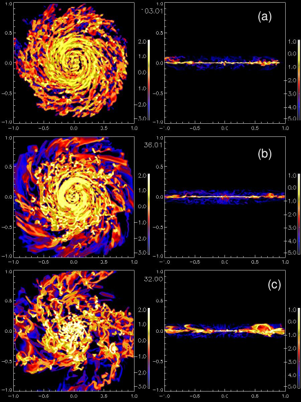
Figure 1.— Surface sections of the density distribution of the gas in models with different initial density (model A, B, and D). x-y and x-z planes are shown. Unit of length is kpc. (a) model A ($\rho_{i}=5M_{\odot}$ pc^-3, $t=103$ Myr), (b) model B ($\rho_{i}=10M_{\odot}$ pc^-3, $t=36$ Myr), and (c) model D ($\rho_{i}=50M_{\odot}$ pc^-3, $t=32$ Myr).

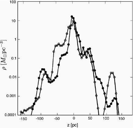
Figure 2.— Vertical density structure of model D. Two lines represent density averaged for x-direction (black dots) and y-direction (open circles).

Figure 3.— Time evolution of density PDF for the whole computational volume for model D. The lines represent the PDF at $t=3,10,16,21$, and 43 Myr (thick solid line). The vertical axis is the number fraction of grid cells for the density. The unit of density is $M_{\odot}$ pc^-3.

Figure 4.— Density PDF for four sub-regions in model D. Solid line is a thin disk ($|z|\leq 10$ pc), dotted line is a inner disk ($10\leq z\leq 20$ pc and $|x,y|\leq 0.38$ kpc), dashed line is a halo ($30\leq z\leq$ 160 pc), where $z=0$ is the galactic plane. The two solid curves are a log-normal function with $\sigma_{10}=1.273$, $\log(\rho_{0})=-1.2$ and $\alpha=$ 0.02 (disk), and $\sigma_{10}=1.308$, $\log(\rho_{0})=-1.5$ and $\alpha=$ 0.2 (the whole region).

Figure 5.— Same as Fig. 4, but for model B.

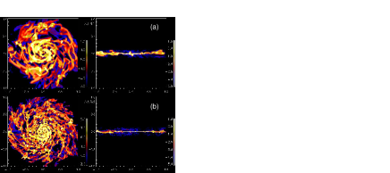
Figure 6.— Density structures of model C with two deferent resolutions. A temperature floor depending on the resolution: (a) $\Delta=10$ pc, and (b) $\Delta=5$ pc. $T_{\rm min}=35$ K ($\rho_{i}/10M_{\odot}$ pc^-3) ($\Delta$/5 pc)² is assumed to ensure that the Jeans unstable is resolved.

Figure 7.— Density PDF for model C with two deferent resolutions. (a) $\Delta=10$ pc, (b) $\Delta=5$ pc. Three lines are PDF for the whole computational box, disk, and the inner disk (dotted line).

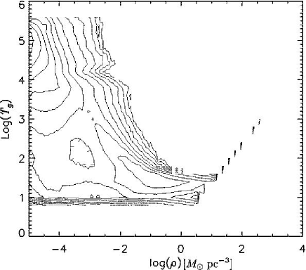
Figure 8.— Phase diagram of model D at $t=43$ Myr. Contours represent log-scaled volumes.

Figure 9.— Mass-weighted PDF for (a) model D, (b) model C, (c) model B, and (d) model A. Unit of density is $M_{\odot}$ pc^-3. In the log-normal fit, $\rho_{0,M}=\rho_{0}e^{\sigma^{2}}$ (eq. (6)) and $\sigma$ for the volume-weighted PDF (table 1) are used. The cut-off at high density in each plot is caused by the resolution limit.

Figure 10.— Effective pressure-density diagram of model E. Two power-laws are $p_{\rm eff}\propto\rho^{2/3}$ and $p_{\rm eff}\propto\rho^{4/3}$. $p_{\rm eff}\equiv p_{\rm th}+\rho v_{t}^{2}$, where $p_{\rm th}$ is the thermal pressure and $v_{t}$ is turbulent velocity of the medium. The contours represent log-scaled volumes for given density and $p_{\rm eff}$.

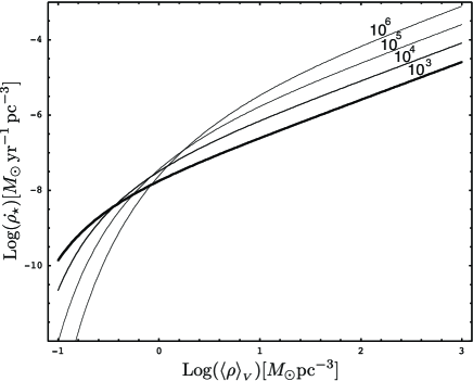
Figure 11.— Star formation rate ($\dot{\rho_{\star}}$) as a function of volume average density ($\bar{\rho}$) for 0.01. $\rho_{0}=1$ cm^-3 is assumed. Four curves are plotted for $\delta_{c}=10^{3}$ (thick solid line), $10^{4},10^{5}$ and $10^{6}$ (from thick to thin lines) are plotted.

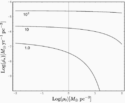
Figure 12.— Star formation rate ($\dot{\rho_{\star}}$) as a function of the characteristic density of the LN-PDF ($\rho_{0}$) for different average density $\langle\rho\rangle_{V}=10^{2},10$, and $1M_{\odot}$ pc^-3. $\delta_{c}=10^{4}$ is assumed.

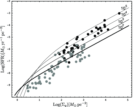
Figure 13.— Comparison between our models and observed surface star formation rate in terms of surface gas density. Black dots are starburst galaxies in Kennicutt (1998) and gray dots are normal galaxies in Komugi et al. (2005). Four curves are SFR for $\delta_{c}=10^{2}$ (thick solid line), $10^{3},10^{4}$ and $10^{5}$. $\alpha=0.1$, $\rho_{0}=1.0$, and $\epsilon_{c}=0.01$ are assumed.

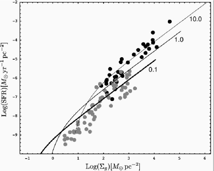
Figure 14.— Same as Fig. 13, but for dependence of characteristic density of LN-PDF, $\rho_{0}=0.1$ (thick solid line), 1 and $10M_{\odot}$ pc^-3. $\alpha=0.1$, $\delta_{c}=10^{3}$, and $\epsilon_{c}=0.01$ are assumed.

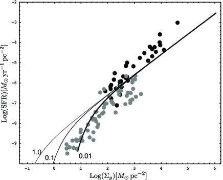
Figure 15.— Same as Fig. 13, but for dependence of fraction of LN part, $\alpha=0.01$ (thick solid line), 0.1, and 1.0. $\rho_{0}=1.0$, $\delta_{c}=10^{3}$, and $\epsilon_{c}=0.01$ are assumed.

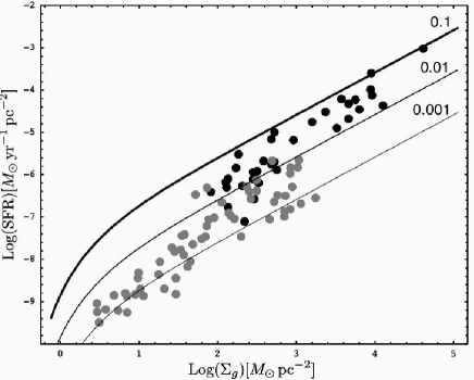
Figure 16.— Same as Fig. 13, but for the best-fit model ($\rho_{0}=1.0,\alpha=0.1,$ and $\delta_{c}=10^{3}$). Three curves are for $\epsilon_{c}=0.1$ (thick solid line), 0.01 and 0.001.

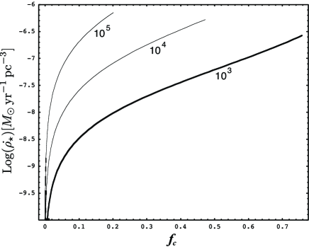
Figure 17.— SFR as a function of a fraction of high density gas $f_{c}$. Three curves are plotted for $\delta_{c}=10^{3}$ (thick line), $10^{4}$, and $10^{5}$. $\epsilon_{c}=0.1$ and $\alpha=0.1$ are assumed.

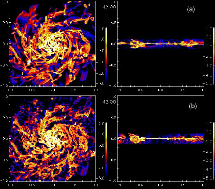
Figure 18.— Same as Fig. 1, but comparison between models with and without energy feed back from supernovae. (a) model D, (b) model D, but with supernova explosions at a rate of 1.5$\times 10^{-3}$ yr^-1 kpc^-2.

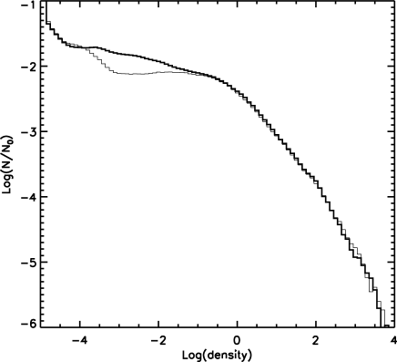
Figure 19.— PDF in models with and without energy feedback from supernovae. Thin line is model D, and thick line is model D, but with supernova explosions at a rate of 1.5$\times 10^{-3}$ yr^-1 kpc^-2.

References

- de Avillez (2000) de Avillez, M. A. 2000, MNRAS, 315, 479
- Binney & Tremain (1987) Binney, J., Tremaine, S., 1997, “Galactic Dynamics”, Princeton Univ. Press, Princeton, New Jersey M. 1985, A&A, 150, 327
- Bania & Lyon (1980) Bania, T. M. & Lyon, J. G., 1980, ApJ, 239, 173
- Elmegreen (2002) Elmegreen, B. G. 2002, ApJ, 577, 206
- Fukui et al. (2001) Fukui, Y., Mizuno, N., Yamaguchi, R., Mizuno, A., & Onishi, T. 2001, PASJ, 53, L41
- Gao & Solomon (2004) Gao, Y., & Solomon, P. M. 2004, ApJS, 152, 63
- Gerritsen & Icke (1997) Gerritsen, J. P. E., Icke, V., 1997, A&Ap, 325, 972
- Goldreich & Lynden-Bell (1965) Goldreich, P., & Lynden-Bell, D. 1965, MNRAS, 130, 125
- Hockney & Eastwood (1981) Hockney, R. W., Eastwood, J. W. 1981, Computer Simulation Using Particles (New York : McGraw Hill)
- Kauffmann et al. (2003) Kauffmann, G., et al. 2003, MNRAS, 341, 54
- Kennicutt (1998) Kennicutt, R., 1998, ApJ, 498, 541
- Kim et al. (2003) Kim, S., Staveley-Smith, L., Dopita, M. A., Sault, R. J., Freeman, K. C., Lee, Y., & Chu, Y.-H. 2003, ApJS, 148, 473
- Koda et al. (2005) Koda, J., Okuda, T., Nakanishi, K., Kohno, K., Ishizuki, S., Kuno, N., & Okumura, S. K. 2005, A&A, 431, 887
- Kodama et al. (2004) Kodama, T., et al. 2004, MNRAS, 350, 1005
- Komugi et al. (2005) Komugi, S., Sofue, Y., Nakanishi, H., Onodera, S., & Egusa, F., 2005, PASJ, 57, 733
- Kravtsov (2003) Kravtsov, A. V. 2003, ApJ, 590, L1
- Kravtsov & Gnedin (2005) Kravtsov, A. V., & Gnedin, O. Y. 2005, ApJ, 623, 650
- Krumholz & McKee (2005) Krumholz, M. R., & McKee, C. F. 2005, ApJ, 630, 250
- Larson (1981) Larson, R. B. 1981, MNRAS, 194, 809
- Li, Mac Low, & Klessen (2006) Li, Y., Mac Low, M.-M., & Klessen, R. S. 2006, ApJ, 639, 879
- Liou & Steffen (1993) Liou, M., Steffen, C., 1993, J.Comp.Phys., 107,23
- Mac Low (1999) Mac Low, M.-M. 1999, ApJ, 524, 169
- Martin et al. (2004) Martin, C. L., Walsh, W. M., Xiao, K., Lane, A. P., Walker, C. K., & Stark, A. A. 2004, ApJS, 150, 239
- Martin & Kennicutt (2001) Martin, C. L., & Kennicutt, R. C. 2001, ApJ, 555, 301
- Myers (1978) Myers, P. C. 1978, ApJ, 225, 380
- Nordlund & Padoan (1998) Nordlund, A., & Padoan, P., 1998, in Interstellar Turbulence, ed. J.Franco & A. Carraminana, Cambridge, Cambridge Univ. Press, p. 218
- Ostriker et al. (2001) Ostriker, E. C., Stone, J. M., & Gammie, C. F. 2001, ApJ, 546, 980
- Padoan, Nordlund, & Johns (1997) Padoan,P., Nordlund, A., & Johns,B.J.T. 1997, MNRAS, 288,145
- Rosen & Bregman (1995) Rosen, A., Bregman, J.N., 1995,ApJ, 440, 634
- Scalo et al. (1998) Scalo, J., Vzquez-Semadeni, E., Chappell, D.,Passot, T., 1998, ApJ, 504,835
- Scoville & Solomon (1974) Scoville, N. Z. & Solomon, P. M. 1974, ApJ, 187, L67
- Schmidt (1959) Schmidt, M. 1959, ApJ, 129, 243
- Slyz et al. (2005) Slyz, A. D., Devriendt, J. E. G., Bryan, G., & Silk, J. 2005, MNRAS, 356, 737
- Spaans & Norman (1997) Spaans, M., Norman C., 1997, ApJ, 483, 87
- Sánchez-Salcedo (2001) Sánchez-Salcedo, F. J. 2001, ApJ, 563, 867
- Susa & Umemura (2004) Susa, H., & Umemura, M. 2004, ApJ, 610, L5
- Tasker & Bryan (2006) Tasker, E. J., & Bryan, G. L. 2006, ApJ, 641, 878
- Tozzi, et al. (2006) Tozzi, P., et al. 2006 astro-ph/0602127
- van Leer (1977) van Leer, B., 1977, J.Comp.Phys., 32, 101
- Vazquez-Semadeni (1994) Vzquez-Semadeni, E. 1994, ApJ, 423, 681
- Vazquez-Semadeni, Gazol, & Scalo (2000) Vzquez-Semadeni, E., Gazol, A.& Scalo, J. 2000, ApJ, 540, 271 98
- Wong & Blitz (2002) Wong, T., & Blitz, L. 2002, ApJ, 569, 157
- Wada (2001) Wada, K. 2001, ApJ, 559, L41 (W01)
- Wada & Norman (1999) Wada, K. & Norman, C. A. 1999, ApJ, 516, L13
- Wada & Norman (2001) Wada, K. & Norman, C. A. 2001, ApJ, 547, 172 (WN01)
- Wada & Norman (2002) Wada, K. & Norman, C. A. 2002, ApJ, 566, L21
- Wada, Spaans, & Kim (2000) Wada, K., Spaans, M., & Kim, S. 2000, ApJ, 540, 797
- Wada, Meurer, & Norman (2002) Wada, K., Meurer, G., & Norman, C. A. 2002, ApJ, 577, 197
- Wada, & Tomisaka (2005) Wada, K., Tomisaka, K. 2005, ApJ, 619, 93
- Yamaguchi et al. (2001) Yamaguchi, R., et al. 2001, PASJ, 53, 985