Constraints on Dark Energy from Supernovae, $\gamma$-ray bursts, Acoustic Oscillations, Nucleosynthesis and Large Scale Structure and the Hubble constant

Abstract

The luminosity distance vs. redshift law is now measured using supernovae and $\gamma$-ray bursts, and the angular size distance is measured at the surface of last scattering by the CMB and at $z=0.35$ by baryon acoustic oscillations. In this paper this data is fit to models for the equation of state with $w=-1$, $w=\;$constant, and $w(z)=w_{0}+w_{a}(1-a)$. The last model is poorly constrained by the distance data, leading to unphysical solutions where the dark energy dominates at early times unless the large scale structure and acoustic scale constraints are modified to allow for early time dark energy effects. A flat $\Lambda$CDM model is consistent with all the data.

1 INTRODUCTION

Wood-Vasey et al. (2007) recently published supernova data from the ESSENCE project, while Riess et al. (2007) have published a large sample of supernovae from the SNLS project (Astier et al. 2006), the HST, and Hi-z Supernova Team. Schaefer (2006) has published a sample of $\gamma$-ray burst distances. While GRBs give much less accurate distances than supernovae, they extend to much higher redshifts and the GRB data helps to distinguish between non-flat geometries and equations of state with $w\neq-1$ which both affect the distance-redshift law at ${\cal O}(z^{3})$ for low redshift.

The analysis of Wood-Vasey et al. (2007) plotted contours of $w$ and $w_{a}$, based only on a subset of the supernova data used here and a prior on $\Omega_{M}$. These contours extended into the region where the dark energy dominated the density at the surface of last scattering or during nucleosynthesis. Li et al. (2006) added GRBs and large scale structure data to the SNe data but still show contours extending into the early dark energy domination region. Both Barger et al. (2006) and Riess et al. (2007) used $w(z)$ laws in which the deviation of $w$ from $-1$ was terminated for $z>1.8$, beyond the redshift of the most distant supernova in the sample, but this is an arbitrary limit which would have to modified to allow for GRBs. Alam, Sahni & Starobinsky (2006) analyzed the SNe data using a quadratic polynomial in $(1+z)$ as the form for $\rho_{DE}$. This form for $\rho_{DE}$ will never be dominant at early times since the matter density varies like $(1+z)^{3}$. Davis et al. (2007) have analyzed a subset of the combined supernovae, and have used an approximation to the CMB acoustic peak constraint that fails when dark energy dominates at high $z$. The part of parameter space where dark energy dominates at high $z$ obviously should be excluded, and I show in this paper that appropriate modifications to the standard formulae for the acoustic scale, the $\Gamma$ parameter, and Big Bang nucleosynthesis (BBNS) to allow for the possible importance dark energy at $z\approx 10^{9}$ or $z\approx 10^{3}$ will lead to this exclusion automatically. The BBNS, acoustic scale and $\Gamma$ limits are given in general forms involving $\rho_{DE}(z)$, which can be used for any form of the equation of state. But the $w=w_{\circ}+w_{a}(1-a)$ form adopted by the Dark Energy Task Force report (Albrecht et al. 2006) is used for all the specific plots in this paper. This form can be used for all redshifts without introducing a redshift cutoff which would be a new and otherwise unnecessary parameter.

Table 1: Mean distance modulus relative to a Milne model for the 358 supernovae in Riess et al. (2007) Gold+Silver and Wood-Vasey et al. (2007).

$\langle z\rangle$	$\langle\Delta\mu\rangle$	$z_{min}$	$z_{max}$	$N$
0.0159	$-0.052\pm 0.118$	0.007	0.024	37
0.0376	$0.004\pm 0.057$	0.024	0.058	37
0.0947	$0.103\pm 0.075$	0.061	0.160	12
0.2207	$0.110\pm 0.062$	0.172	0.268	14
0.3299	$0.096\pm 0.037$	0.274	0.371	36
0.4222	$0.170\pm 0.037$	0.374	0.455	37
0.4841	$0.245\pm 0.037$	0.459	0.511	37
0.5530	$0.169\pm 0.034$	0.514	0.610	37
0.6550	$0.100\pm 0.036$	0.612	0.710	31
0.7747	$0.054\pm 0.053$	0.719	0.818	21
0.8590	$0.055\pm 0.064$	0.822	0.910	20
0.9661	$0.047\pm 0.068$	0.927	1.020	21
1.1140	$0.017\pm 0.118$	1.056	1.140	4
1.2228	$-0.087\pm 0.127$	1.190	1.265	5
1.3353	$-0.151\pm 0.100$	1.300	1.390	6
1.4000	$0.037\pm 0.810$	1.400	1.400	1
1.5510	$-0.490\pm 0.320$	1.551	1.551	1
1.7550	$-0.599\pm 0.350$	1.755	1.755	1

2 OBSERVATIONS

2.1 Supernovae

Table 2: Mean distance modulus relative to a Milne model for 272 supernovae in Riess et al. (2007) Gold and Wood-Vasey et al. (2007).

$\langle z\rangle$	$\langle\Delta\mu\rangle$	$z_{min}$	$z_{max}$	$N$
0.0169	$-0.035\pm 0.125$	0.010	0.025	29
0.0361	$0.024\pm 0.067$	0.025	0.053	29
0.0776	$0.074\pm 0.080$	0.056	0.124	10
0.2032	$0.123\pm 0.073$	0.159	0.249	10
0.3196	$0.105\pm 0.042$	0.263	0.363	27
0.4149	$0.144\pm 0.039$	0.368	0.450	29
0.4808	$0.203\pm 0.040$	0.455	0.508	29
0.5514	$0.139\pm 0.039$	0.510	0.604	29
0.6475	$0.119\pm 0.038$	0.610	0.707	25
0.7888	$0.058\pm 0.059$	0.730	0.830	18
0.8666	$0.007\pm 0.081$	0.832	0.905	10
0.9696	$0.035\pm 0.076$	0.935	1.020	14
1.1140	$0.017\pm 0.118$	1.056	1.140	4
1.2197	$0.081\pm 0.143$	1.199	1.230	3
1.3410	$-0.163\pm 0.105$	1.300	1.390	5
1.7550	$-0.599\pm 0.350$	1.755	1.755	1

Table 3: Mean distance modulus relative to a Milne model for 69 GRBs in Schaefer (2007).

$\langle z\rangle$	$\langle\Delta\mu\rangle$	$z_{min}$	$z_{max}$	$N$
0.2100	$0.453\pm 0.362$	0.170	0.250	2
0.4967	$0.458\pm 0.289$	0.430	0.610	3
0.7350	$0.479\pm 0.217$	0.650	0.830	8
0.9187	$-0.090\pm 0.171$	0.840	1.020	8
1.2083	$0.173\pm 0.263$	1.060	1.310	6
1.5275	$-0.202\pm 0.175$	1.440	1.620	8
2.0217	$-0.141\pm 0.257$	1.710	2.200	6
2.4825	$-0.117\pm 0.211$	2.300	2.680	8
3.1463	$-0.785\pm 0.215$	2.820	3.370	8
3.8243	$-0.573\pm 0.247$	3.420	4.270	7
4.6033	$-0.946\pm 0.412$	4.410	4.900	3
6.4450	$-1.100\pm 0.463$	6.290	6.600	2

The distance modulus vs. redshift data from Riess et al. (2007) were taken from the Web site provided by Riess. The distance moduli and redshifts for the ESSENCE supernovae were extracted from Table 9 in the Latex file for astro-ph/0701041 (Wood-Vasey et al. 2007). Typically different groups analyze supernovae with different assumptions about the Hubble constant or equivalently the absolute magnitude ${\cal M}$ of a canonical SN Ia with a nominal decay rate. In order to combine the new supernovae from ESSENCE with the Riess et al. sample, it was necessary to check the relative normalization of the two data sets using the 93 objects they have in common. Figure 1 shows the comparison. The scatter in the differential distance moduli is $0.2$ mag 1$\sigma$, which seems unusually high, and the median difference in $\mu$ is 0.022 mag which is consistent with the standard deviation of the mean given the scatter. Objects which are not in the Riess et al. sample but which had successful fits with $\chi^{2}$ per degree of freedom $<7$ were added to the Riess et al. sample, with the 0.022 mag added to $\mu$, and an intrinsic scatter of $0.10$ mag added in quadrature to $\sigma_{\mu}$. This gives a total sample of 358 SNe. I have binned the SNe into bins containing $<2+N_{tot}/10$ objects and widths less than 0.1 in redshift. An empty Universe model (the Milne model) was first subtracted from the $\mu$ values. The binned values are listed in Table 1. A Hubble constant of 63.8 km/sec/Mpc was used when computing the Milne model, but this value has no effect on the parameter limits computed in this paper. Its only effect is to add a constant to the $\langle\Delta\mu\rangle$ values in the Tables. The mean differential distance modulus in each bin is found by minimizing a modified

$$\chi^{2}=\sum_{i}f((<\Delta\mu>-[\mu_{i}-\mu_{Milne}])/\sigma_{i})$$ (1)

where $f(x)=x^{2}$ for $|x|<2$, or $4|x|-4$ otherwise. The modification deweights extreme outliers. Riess et al. (2007) recommend dropping SNe with redshifts less than 0.023 to avoid a possible “Hubble bubble” seen by Jha et al.(2007), but I have instead used a large velocity error of $\sigma_{v}=1500$ km/sec which gives an extra $\sigma_{\mu}$ of $(5/\ln 10)(\sigma_{v}/cz)$ which is added in quadrature with the tabulated $\sigma_{\mu}$.

Table 2 was constructed the same way but omitting the “Silver” objects in Riess et al. (2007).

The binned values from Tables 1 and 2 are shown in Figure 2 along with the flat $\Lambda$CDM model that best fits the Hubble diagram data alone. This model has $\Omega_{M}=0.369$. There is an excursion around $z=0.5$ that can be seen clearly in the binned supernova data. A simple 3 parameter fit to this bump gives a $\Delta\chi^{2}$ of 15 in the total sample, but only 6 if the “Silver” SNe are excluded.

2.2 GRBs

Schaefer (2007) has given a sample of 69 GRBs with redshifts and distance moduli. These values have been binned as well, but with bin widths $<0.1(1+z_{min}+z_{max})$. The binned values are listed in Table 3. In constructing the Table, a Milne model with a Hubble constant of 72 km/sec/Mpc was subtracted from the individual distance moduli before minimizing the modified $\chi^{2}$. Figure 3 shows the binned data from both the GRBs and the supernovae.

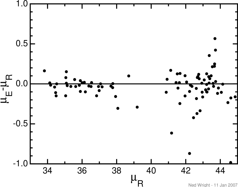
Figure 1: Difference in distance moduli for objects common to Wood-Vasey et al. (2007) ($\mu_{E}$) and Riess et al. (2007) ($\mu_{R}$). The RMS scatter is 0.2 mag.

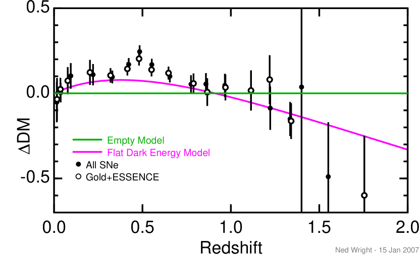
Figure 2: Binned supernova data vs. redshift compared to a flat $\Lambda$CDM model with $\Omega_{M}=0.369$. The filled circles are binned points from the full dataset, while the open circles have omitted the “Silver” subset.

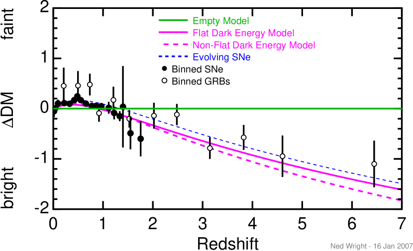
Figure 3: Binned supernova and GRB data vs. redshift compared to a flat $\Lambda$CDM model with $\Omega_{M}=0.369$, and non-flat $\Lambda$CDM model with $\Omega_{M}=0.416$ and $\Omega_{tot}=1.115$, and an exponentially evolving model in a $\Omega_{M}=1$ model (Wright 2002).

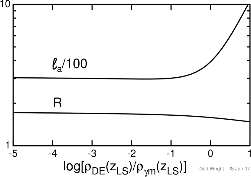
Figure 4: The stretch parameter $R$ and the acoustic scale $\ell_{a}$ as a function of the ratio of dark energy density to matter plus radiation density at $z_{LS}$. These curves were evaluated for flat models by varying $w^{\prime}$, setting $w_{0}=-0.922-0.309w^{\prime}$ and then adjusting $\Omega_{M}$ to minimize the $\chi^{2}$ from the supernovae fit plus the simple $\Omega_{M}=0.296\pm 0.029$ prior.

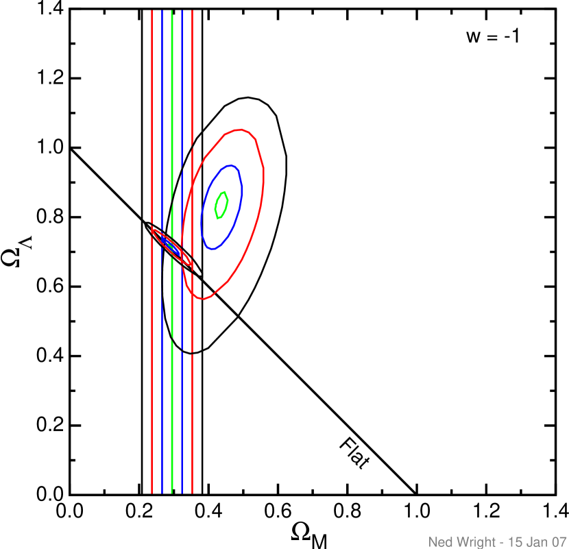
Figure 5: Contours of $\chi^{2}$ in the $\Omega_{M}$-$\Omega_{\Lambda}$ plane when the dark energy is assumed to be a cosmological constant with $w=-1$. The large ellipses use only the Hubble diagram data from the supernovae and the GRBs. The small ellipses near the “Flat” line use only the CMB acoustic scale and the baryon acoustic distance ratio. Contours are drawn for $\Delta\chi^{2}=0.1$, 1, 4, and 9. The vertical lines show -3 …+3 $\sigma$ for the $\Omega_{M}$ prior derived from $\Gamma$, $H_{\circ}$ and $\omega_{M}$.

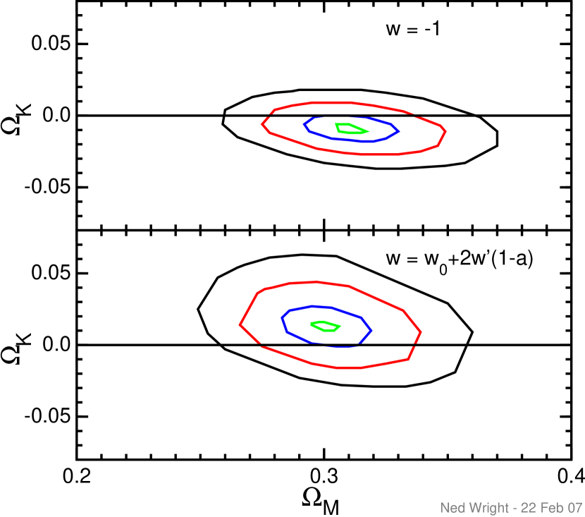
Figure 6: Contours of $\chi^{2}$ in the $\Omega_{M}$-$\Omega_{K}$ plane. In the lower panel the dark energy is allowed to vary as $w(z)=w_{\circ}+2w^{\prime}(1-a)$, using all constraints and datasets. A flat model is consistent with the data, and the best fit is very slight open. In the upper panel $w=-1$, and a flat model is again consistent but the best fit is slightly closed.

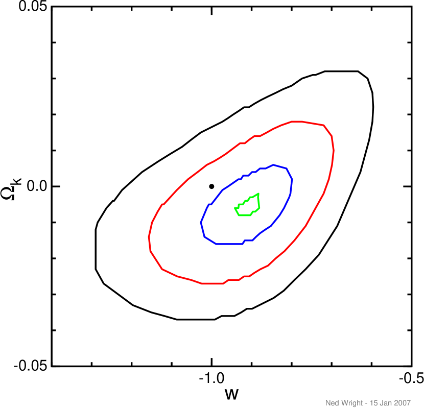
Figure 7: Contours of $\Delta\chi^{2}$ in the $w$, $\Omega_{K}$ plane, with $w^{\prime}$ fixed at zero and $\Omega_{M}$ adjusted to minimize $\chi^{2}$ at each point. The black dot shows the flat $\Lambda$CDM model, which has 2 fewer free parameters and less than two units of $\Delta\chi^{2}$.

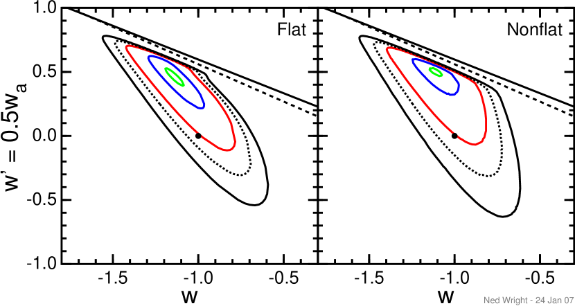
Figure 8: Contours of $\Delta\chi^{2}$ in the $w$, $w^{\prime}$ plane, using all constraints and datasets. The dotted contour shows the $\Delta\chi^{2}=6.17$ used in the DETF Figure of Merit. On the left the curvature $\Omega_{K}$ is fixed at zero and $\Omega_{M}$ is adjusted to minimize $\chi^{2}$ at each point. On the right both $\Omega_{M}$ and $\Omega_{K}$ are adjusted to minimize $\chi^{2}$ at each point. The black dot shows the cosmological constant $w=-1$. The dashed diagonal line shows where the dark energy is equal to the matter plus radiation density at last scattering. The solid diagonal line shows the 3 $\sigma$ limit on the stretch parameter $S^{BBNS}$.

2.3 Hubble Constant

The Hubble constant largely cancels out in analyses of supernovae and $\gamma$-ray burst distances. But the Hubble constant does enter into converting the $\Gamma$ parameter ($\Omega_{M}h$) into a prior on $\Omega_{M}$. The Hubble constant data used in this paper comes from Freedman et al. (2001), the DIRECT project double-lined eclipsing binary in M33 (Bonanos et al. 2006), Cepheids in the nuclear maser ring galaxy M106 (Macri et al. 2006), and the Sunyaev-Zeldovich effect (Bonamente et al. 2006). These papers gave values of $72\pm 8$, $61\pm 4$, $74\pm 7$ and $77\pm 10$ km/sec/Mpc. Assuming that the uncertainties in these determinations are uncorrelated and equal to 10 km/sec/Mpc after allowing for systematics, the average value for $H_{\circ}$ is $71\pm 5$ km/sec/Mpc. This average is consistent with the $74\pm 4(stat)\pm 5(sys)$ km/sec/Mpc from Riess et al. (2005).

2.4 Matter Density

The matter density $\Omega_{M}h^{2}$ is fairly well determined by fitting the CMB power spectrum. In this paper the non-flat $\Lambda$CDM chain (ocdm_wmap_1.txt) at the LAMBDA data center has been used to determine average values for parameters. This chain gives $\omega_{M}=\Omega_{M}h^{2}=0.1289\pm 0.0079$. The baryonic density is also well determined, with $\omega_{B}=\Omega_{B}h^{2}=0.02178\pm 0.00072$.

2.5 Large Scale Structure

Large scale structure data comes from the “big bend” in the power spectrum $P(k)$. This has been measured by two large galaxy surveys: the SDSS and the 2dF. The SDSS gives a value for $\Gamma=\Omega_{M}h=0.213\pm 0.0233$ (Tegmark et al. 2004), while the 2dF gives (Cole et al. 2005)

$$\Omega_{M}h=\Gamma_{true}=0.168\pm 0.016+0.3(1-n_{s})+1.2\Omega_{\nu}/\Omega_{M}$$ (2)

I assume that the Tegmark et al. value uses $n_{s}=1$ and $\Omega_{\nu}=0$, and that it has the same sensitivity to these parameters as the 2dF. The combination of these two values gives a $\chi^{2}=2.6$ for 1 degree of freedom. While this is higher than the expected value of 1, it is certainly not high enough to trigger grave concerns. The neutrino density is uncertain but the minimal hierarchical mass pattern gives $\Omega_{\nu}/\Omega_{M}\approx 0.004$ while the WMAP 3 year data give $n_{s}=0.951\pm 0.017$ (Spergel et al. 2007). With these values the corrected weighted mean $\Gamma$ is $0.209\pm 0.014$.

2.6 Acoustic Oscillations

The most important parameter from the CMB data is the acoustic scale. In this paper the stretch parameter $R=\Omega_{M}^{1/2}H_{\circ}(1+z_{LS})D_{A}(z_{LS})/c$ (Bond, Efstathiou & Tegmark 1997; Wang & Mukherjee 2006) is not used, but the acoustic scale $\ell_{a}$ evaluated at the mean baryon and dark matter densities is used in its place. The acoustic scale is defined as (Page et al. 2003)

$$\ell_{a}=\frac{\pi(1+z_{LS})D_{A}(z_{LS})}{\int_{0}^{1/(1+z_{LS})}c_{s}da/(a\dot{a})}$$ (3)

where $z_{LS}$ is last scattering, $c_{s}$ is the sound speed, $a$ is the scale factor, $\dot{a}$ is its time derivative, and $D_{A}$ is the angular size distance. The stretch parameter $R$ has a different normalization and approximates the denominator as $\propto\Omega_{M}^{-1/2}$, which is not a good approximation when the dark energy is significant at $z_{LS}$. $\ell_{a}$ is very well determined by the CMB data, with $\ell_{a}=303.14\pm 1.04$ in the non-flat $\Lambda$CDM chain. There are correlated deviations in $\omega_{B}$, $\omega_{M}$, $\Omega_{\Lambda}$ and $\Omega_{k}$ that produce correlated deviations in the numerator and denominator of Eq(3) which cancel out in the ratio. In this paper the full fit to the CMB data is not performed, but the baryon and CDM densities are fixed at their mean values. With this simplification, the determination of the acoustic scale loosens to $\ell_{a}=302.97\pm 4.14$ because the deviations in the numerator are still present. The relative accuracy of $\ell_{a}$ with fixed $\omega_{B}$ and $\omega_{M}$ is the same as the relative accuracy of $R$. The main reason to use $\ell_{a}$ instead of $R$ is that it is clear how $\ell_{a}$ is modified when the dark energy is important at last scattering. Figure 4 shows that $\ell_{a}$ shifts a great deal when the dark energy density is greater than the radiation plus matter density at recombination, while the change in $R$ is smaller and in the wrong direction.

The CMB also provides the matter density $\omega_{M}$ used as part of the large scale structure analysis. For models far from the geometric degeneracy line, a full fit to the CMB power spectrum will compensate for an incorrect distance to the surface of last scattering by changing $\omega_{M}$ and $\omega_{B}$ to give a different value of the sound horizon at last scattering, but this effect has not been been included here. Ultimately a full fit to all the data should be performed, and the CMB is both the most informative and the most computationally intensive of all the datasets. Spergel et al. (2007) has some limits on $w$, but not on the $w,w^{\prime}$ plane, and does not include either the Riess et al. (2007) and Wood-Vasey et al. (2007) increments to the supernova data or the GRB data.

The second major input involving acoustic oscillations comes from the baryon acoustic oscillations detected by Eisenstein et al.  (2005). In this paper we use the ratio of the distance $D_{V}(0.35)$ at $z=0.35$ to the tangential distance at last scattering,

$$R_{0.35}=\frac{D_{V}(0.35)}{(1+z_{LS})D_{A}(z_{LS})}$$ (4)

This ratio is easily computed even when the dark energy is significant at last scattering. The ratio is also slightly more precise than the $A$ parameter since the scatter induced by the uncertainty in $\omega_{B}$ and $\omega_{M}$ cancels out in the ratio. The $A$ parameter also uses the approximation that the sound travel distance is $\propto\Omega_{M}^{-1/2}$ which fails when dark energy dominates early. Finally, $A/R$ is exactly proportional to $D_{V}(0.35)/[(1+z_{LS})D_{A}(z_{LS})]$. Using both $A$ and the distance ratio amounts to double counting the baryon acoustic oscillations.

The redshift of last scattering, $z_{LS}$, is essentially independent of both the baryon density and the expansion rate because the electron density is $n_{e}\propto H(z)/\alpha(T)$ while the optical depth is $\tau\propto\sigma_{T}n_{e}c/H(z)\propto\sigma_{T}/\alpha(T)$ where $\sigma_{T}$ is the scattering cross-section and $\alpha$ is the recombination coefficient. Hence $z_{LS}=1089$ is used for all calculations in this paper.

2.7 Big Bang Nucleosynthesis

Steigman (2006) has analyzed the light element abundances and obtained limits on a stretch factor $S^{BBNS}=(1+\rho_{DE}/\rho_{\gamma+m+k})^{1/2}$. The limits are $S^{BBNS}=0.942\pm 0.030$. This means that at 3 $\sigma$ the dark energy density must be less than 6.4% of the radiation density at the redshift of nucleosynthesis, $z\approx 10^{9}$.

2.8 Expansion Rate at Last Scattering

Zahn & Zaldarriaga (2003) have shown that even though $H(z)$ cancels out in determining $z_{LS}$, the width in conformal time of the transition from opaque to transparent can be determined using the CMB TT and TE power spectra, and that this can give a stretch factor similar to the BBNS stretch factor. Zahn & Zaldarriaga interpret this in terms of varying Newton’s constant $G$, but it really depends on $\sqrt{G\rho}$. Interpreting the limit in Zahn & Zaldarriaga in terms of the dark energy density instead of a changing $G$ gives $S^{LS}=(1+\rho_{DE}/\rho_{\gamma+m+k})^{1/2}=1.749\pm 0.471$ at $z_{LS}$. With the first year WMAP data this improved to $1.04\pm 0.24$ (Zahn, private communication).

3 ANALYSIS

All of the analyses in this paper depend on the expansion history and geometry of the Universe. The expansion history can be calculated using

$$\dot{a}=H_{\circ}\sqrt{\Omega_{M}/a+\Omega_{R}/a^{2}+\Omega_{K}+\Omega_{DE}[\rho_{DE}(z)/\rho_{DE}(0)]a^{2}}$$ (5)

The dark energy density as a function of redshift is computed using the $w=w_{0}+w_{a}(1-a)$ formula (Chevallier & Polarski, 2001). Following Linder (2003) I set $w^{\prime}=w_{a}/2$. This then gives

$$\frac{\rho_{DE}(z)}{\rho_{DE}(0)}=(1+z)^{3+3w_{0}+6w^{\prime}}\exp\left(\frac{-6w^{\prime}z}{1+z}\right)$$ (6)

The calculation of angular size and luminosity distances then follows Wright (2006).

Note that the binned distance moduli were not used for the analysis. Thus the Hubble constants used when producing the binned data tables are irrelevant in the analysis. But both the supernovae and the GRBs have an associated “nuisance” parameter, ${\cal M}_{SN}$ and ${\cal M}_{GRB}$, which are adjusted to give the best modified $\chi^{2}$ at every position in the $\{\Omega_{M},\Omega_{k},w,w^{\prime}\}$ parameter space. Thus

$$\chi^{2}(\Omega_{M},\Omega_{k},w,w^{\prime}) = \min_{{\cal M}}\sum_{i}f((\mu_{i}-\mu_{c}(z_{i}))/\sigma_{i})$$

with

$$\mu_{c}(z) = {\cal M}+5\log(D_{L}(z;\Omega_{M},\Omega_{k},w,w^{\prime}))$$ (7)

The form in Eq(7) is used twice, once for the supernovae giving $\chi^{2}_{SN}$ and once for the GRBs giving $\chi^{2}_{GRB}$. Contours of the sum of these two terms are shown in Figure 5.

The acoustic scale quantities $\ell_{a}$ and $R_{0.35}$ give a contribution to the overall $\chi^{2}$ of

$$\chi^{2}_{a}(\Omega_{M},\Omega_{k},w,w^{\prime}) = \hat{f}(\ell_{a}(\Omega_{M},\Omega_{k},w,w^{\prime})-\ell_{a,obs})/\sigma(\ell_{a}))$$ (8)

$$+ \hat{f}(R_{0.35}(\Omega_{M},\Omega_{k},w,w^{\prime})-R_{0.35,obs})/\sigma(R_{0.35}),.$$

where $\hat{f}$ is the function from Eq(1) with the transition from quadratic to linear behavior set at $3\sigma$: $\hat{f}(x)=x^{2}$ for $|x|<3$, or $6|x|-9$ otherwise.

Contours of $\chi^{2}_{a}$ are shown in Figure 5.

Normally the data on $\Gamma=\Omega_{M}h$, $H_{\circ}$ and $\Omega_{M}h^{2}$ can be combined to give a prior on $\Omega_{M}$. There is an overdetermined set of equations with variables $\Omega_{M}$ and $h$:

$$\left(\begin{array}[]{cc}1&1\\ 1&2\\ 0&1\end{array}\right)\left(\begin{array}[]{c}\ln(\Omega_{M})\\ \ln(h)\end{array}\right)=\left(\begin{array}[]{c}\ln(0.209)\pm(0.014/0.209)\\ \ln(0.1289)\pm(0.0079/0.1289)\\ \ln(0.71)\pm(0.05/0.71)\end{array}\right)$$ (9)

The least squares solution of these equations gives $H_{\circ}=67.3\pm 3.7$ km/sec/Mpc and $\Omega_{M}=0.296\pm 0.029$. Contours showing this prior are the vertical lines in Figure 5.

But the relationship between $\Gamma=\Omega_{M}h$ and the big bend in $P(k)$ is derived assuming that matter and radiation are the only significant contributors to the density at $z_{eq}$, the redshift of matter-radiation equality. Prior to $z_{eq}$, the Universe is expanding faster than the free-fall time for matter perturbations, so growth is suppressed for fluctuations that are inside the horizon earlier than $z_{eq}$. To allow for the possibility that dark energy contributes, $z_{eq}$ is found using

$$\Omega_{M}(1+z_{eq})^{3}=\Omega_{R}(1+z_{eq})^{4}+\Omega_{K}(1+z_{eq})^{2}+\Omega_{DE}(1+z_{eq})^{3+3w_{0}+6w^{\prime}}\exp\left(\frac{-6w^{\prime}z_{eq}}{1+z_{eq}}\right)$$ (10)

The horizon at $z_{eq}$ is found using

$$D_{eq}=\int_{0}^{1/(1+z_{eq})}\frac{cda}{a\dot{a}}$$ (11)

Then the effective value of $\Gamma$ is $\Gamma_{\mbox{{\small eff}}}=(1602\;\mbox{km/sec})/(H_{\circ}D_{eq})$. By finding the effective $\Gamma_{\mbox{{\small eff}}}$ at two different values for $H_{\circ}$, which leads to two different values for $\Omega_{R}$ since $\Omega_{R}h^{2}$ is fixed by the measurement of $T_{\circ}$, the standard $\Gamma=\Omega_{M}h$ can be replaced by a modified power law function of $h$ which reduces to the standard form except when the dark energy is significant near $z_{eq}$. For example, in the track of models shown in Figure 4, when $\rho_{DE}/\rho_{\gamma m}=0.138$ at $z_{LS}$ one has $\Omega_{M}=0.2983$, $w=-1.098$ and $w^{\prime}=0.570$. These values give $w(z)=0.042$ at $z>>10^{3}$, so the dark energy density grows faster than the matter density but slower than the radiation density at high $z$. For these parameters one finds that $\Gamma_{\mbox{{\small eff}}}=0.171704$ for $h=0.675373$ and $\Gamma_{\mbox{{\small eff}}}=0.188939$ for $h=0.746402$. Fitting a power law function of $h$ gives $\Gamma_{\mbox{{\small eff}}}\approx 0.2499h^{0.95657}$ instead of the standard $0.2983h$. For $h=0.71$ this is a 16% difference which is quite significant compared to the 7% precision of the mean of the $\Gamma$’s from the SDSS and the 2dF. When finding $\chi^{2}$, a weighted mean estimate for $h$ is found using the $\Gamma$, $H_{\circ}$ and $\omega_{m}$ priors. This weighted mean minimizes the $\chi^{2}$ contribution from these three priors, and this minimum is added to the $\chi^{2}$ from the Hubble diagram, CMB, and the BAO. Therefore $h$ becomes a third nuisance parameter. Then

$$\chi^{2}_{\Gamma}(\Omega_{M},\Omega_{k},w,w^{\prime}) = \min_{h}[\hat{f}((\Gamma_{\mbox{{\small eff}}}(\Omega_{M},\Omega_{k},w,w^{\prime},h)-\Gamma_{obs})/\sigma(\Gamma))$$ (12)

$$+ \hat{f}(\Omega_{M}h^{2}-\omega_{M,obs})/\sigma(\omega_{M})+\hat{f}((h-h_{obs})/\sigma(h))]$$

is added to the overall $\chi^{2}$. As the dark energy becomes significant at recombination, $\Omega_{M}$ has to increase to keep the effective $\Gamma$ close to the observed value. If we take the same $w=-1.098$ and $w^{\prime}=0.570$ example discussed above, and adjust $\Omega_{M}$ in flat models to minimize $\chi^{2}_{\Gamma}$ alone, $\Omega_{M}$ increases by $1.5\sigma$ from 0.296 to 0.341. Thus a simple $\Omega_{M}$ prior is not correct when dark energy is significant at $z_{LS}$. Note that $\omega_{M,obs}$, which is derived from the peak heights and trough depths in the CMB angular power spectrum, will be affected by perturbations in the dark energy density, but this effect has not been included in this paper.

It is simple to find the BBNS $S^{BBNS}$ parameter for any point in the $\{\Omega_{M},\Omega_{k},w,w^{\prime}\}$ parameter space, and add an appropriate term to $\chi^{2}$. In doing this calculation I have used $h=\sqrt{\omega_{M}(CMB)/\Omega_{M}}$ for simplicity instead of combining this analysis with the calculation of $\chi^{2}_{\Gamma}$. Since the desired value for $S^{BBNS}$ is slightly less than one, while dark energy can only increase $S^{BBNS}$ above one, the BBNS data act only as an upper limit on $w^{\prime}$. The Zahn & Zaldarriaga limit on dark energy at recombination is handled the same way. This gives a stretch factor term of

$$\chi^{2}_{S} = \hat{f}(S^{BBNS}(\Omega_{M},\Omega_{k},w,w^{\prime})-S^{BBNS}_{obs})/\sigma(S^{BBNS}))$$ (13)

$$+ \hat{f}(S^{LS}(\Omega_{M},\Omega_{k},w,w^{\prime})-S^{LS}_{obs})/\sigma(S^{LS})).$$

The final form for the overall $\chi^{2}$ is

$$\chi^{2}(\Omega_{M},\Omega_{k},w,w^{\prime})=\chi^{2}_{SN}+\chi^{2}_{GRB}+\chi^{2}_{a}+\chi^{2}_{\Gamma}+\chi^{2}_{S}.$$ (14)

Note that a minimization over ${\cal M}_{SN}$ has already been done in computing $\chi^{2}_{SN}$ (see Eqn 7), a minimization over ${\cal M}_{GRB}$ has already been done in computing $\chi^{2}_{GRB}$ , and a minimization over $h$ has already been done in computing $\chi^{2}_{\Gamma}$ (see Eqn 12). Thus the overall $\chi^{2}$ is

$$\chi^{2}(\Omega_{M},\Omega_{k},w,w^{\prime})=\min_{h,{\cal M}_{SN},{\cal M}_{GRB}}\chi^{2}(\Omega_{M},\Omega_{k},w,w^{\prime},h,{\cal M}_{SN},{\cal M}_{GRB})$$ (15)

All of the contour plots in this paper except for Figure 5 show contours of this combined function. Unplotted variables are either fixed at assumed values or minimized over. It is correct to remove nuisance parameters by minimizing $\chi^{2}$ or maximizing the likelihood over them (Cash 1976).

Marginalization by integrating the likelihood over the nuisance parameters is wrong (Wright 1994), although it is allowable to marginalize by integrating over the a posteriori probability density function. But this requires a correct prior distribution for the nuisance parameters. The Monte Carlo Markov chain (MCMC) technique is a useful tool for performing such integrals, but the MCMC thus requires correct priors. As an example, consider Figure 20 of Spergel et al. (2007) which shows the CMB constraint in the $(\Omega_{M},\Omega_{\Lambda})$ plane. This should have a uniform prior in $(\Omega_{M},\Omega_{\Lambda})$, but the chain was computed with a uniform prior in $(\Omega_{\Lambda},\Theta_{s})$, so the chain weights had to be multiplied by the Jacobian of the transformation between $(\Omega_{\Lambda},\Theta_{s})$ and $(\Omega_{M},\Omega_{\Lambda})$ before a subset of the chain was selected for plotting.

Marginalization by minimization avoids the need for a prior on the unplotted variables. The plots in this paper show contours of the likelihood, which are the same as contours of the a posteriori probability density function if one assumes a uniform prior in the plotted variables.

Table 4: $\chi^{2}$ for fitting to 358 SNe, 69 GRBs, $\Gamma$, $H_{\circ}$, $\omega_{M}$, and BBNS. The parameters in the fit are $w$, $w^{\prime}$, $\Omega_{M}$, $\Omega_{K}$, ${\cal M}_{SN}$, ${\cal M}_{GRB}$, and $h$.

Model type	$w_{0}$	$w^{\prime}$	$\Omega_{M}$	$\Omega_{K}$	$\chi^{2}$
flat $\Lambda$CDM	-1	0	0.306	0	427.905
nonflat $\Lambda$CDM	-1	0	0.315	-0.011	426.983
nonflat constant $w$	-0.894	0	0.309	-0.003	426.249
flat varying $w$	-1.126	0.451	0.305	0	423.580
nonflat varying $w$	-1.098	0.506	0.299	+0.015	422.856

4 DISCUSSION

There are a large number of different cuts through the 4 dimensional parameter space that can be plotted, and when different subsets of the data are considered the number of plots multiplies rapidly. The best fit $\chi^{2}$ for some of these combinations are listed in Table 4. Figure 5 shows the $\Omega_{M}$ vs. $\Omega_{\Lambda}$ plane when the dark energy is constrained to be a cosmological constant with $w=-1$. Three data subsets are shown: the supernova and GRB Hubble diagrams, the CMB plus BAO acoustic scale data, and the $\Gamma$, $H_{\circ}$ and $\omega_{M}$ data. Clearly the acoustic scale data give a strong confirmation of the need for dark energy, and a much better constraint on the curvature of the Universe. Using all the data together gives the plot shown in Figure 6. The best fit model is slightly closed with $\Omega_{tot}=1.011$ and $\Omega_{M}=0.315$. The best fit flat $\Lambda$CDM model has less than one more unit of $\chi^{2}$ than the best fit non-flat $\Lambda$CDM model so there is no evidence for spatial curvature from these fits. Figure 6 also shows the effect of allowing $w(z)$ to vary.

Another way to see this is to plot $\chi^{2}$ vs. $w$ and $\Omega_{K}$, as seen in Figure 7. In this plot $w^{\prime}$ is forced to zero, and $\Omega_{M}$ is adjusted to minimize $\chi^{2}$ at each point. This plot is very similar to a comparable plot in Spergel et al. (2007).

The flat $\Lambda$CDM model has only 5 more units of $\chi^{2}$ than a non-flat variable $w$ model with 3 more free parameters. The probability of this occurring by chance alone is over 16%, so this improvement is not significant.

Plots of the $w$ vs. $w^{\prime}$ plane are shown in Figure 8, with and without the assumption of a flat Universe. It is obvious that the contours would have extended to much higher values of $w^{\prime}$ if the nucleosynthesis and acoustic scale constraints had not been used. The tilts of the ellipses below these cutoffs indicate that the pivot redshifts for the priors and datasets used here are $z=0.4$ and $z=0.22$. Values of $w$ at the pivot redshift are close to $-0.9$ which is the best fit when $w^{\prime}$ is forced to zero, as shown in Figure 7.

The Dark Energy Task Force (Albrecht et al. 2006) has defined a Figure of Merit as one over the area of the $\Delta\chi^{2}=6.17$ contour in the $w,w_{a}$ plane. Albrecht et al. said that this contour is a 95% confidence contour, which not exactly correct. It is actually a 95.4% confidence contour to match the 2$\sigma$ confidence of a one dimensional Gaussian (Albrecht, private communication). The FoM for the flat case is 1.59 while for the non-flat case it is 1.39, but both of these cases have run up against the constraints against dark energy domination before last scattering. These constraints have given the non-flat case a bigger boost than the flat case. In fact the area of the $\Delta\chi^{2}=1$ contour is smaller for the non-flat case than the flat case, which shows both the inability of the current data to constrain $w,w_{a}$ and the importance of using the constraints coming from high redshift physics.

5 CONCLUSION

All of the data considered here are consistent with a flat $\Lambda$CDM model with a constant equation of state $w=-1$. The current data, even with well over 300 supernovae, are not adequate for measuring a time variable equation of state with reasonable precision. Serra, Heavens & Melchiorri (2007) and Davis et al. (2007) agree with this conclusion, as do Liddle et al. (2006), Alam et al. (2006) and Li et al. (2006) using earlier and smaller datasets. The current acoustic scale data, seen in the CMB and the baryon oscillations, is giving more precise information about the expansion history of the Universe, but without the dense redshift coverage provided by the supernovae. There appears to be a systematic deviation of the supernovae data from the models around redshifts near 0.5, whose origin is unknown. Since the choice of data subsets affects the size of this deviation it is probably an artifact. Nesseris & Perivolaropoulos (2006) have found systematic differences between the different data sources that went into Riess et al. (2007) dataset, so artifacts are not unlikely. Furthermore the scatter between the distance determinations of identical supernovae by different groups is unexpectedly large. The GRB Hubble diagram is not very precise but it appears to be consistent with the supernova data. The GRB Hubble diagram does help break the degeneracy between $w\neq-1$ and $\Omega_{K}\neq 0$. The 2dF and SDSS values for $\Gamma$ differ by a slightly disturbing amount, so a new and improved measurement of $\Gamma$ would be useful as a tie breaker. The Hubble constant appears to be determined to better than 10% but independent new data would be quite valuable in pinning down $\Omega_{M}$ in combination with $\Gamma$. Better CMB data from Planck should reduce the uncertainty in $\omega_{B}$ and $\omega_{M}$, which will reduce the uncertainty in $R$ or $\ell_{a}$. It is clear that better data of many types will be needed to pin down $w(z)$.

References

- Alam et al. (2006) Alam, U., Sahni, V., & Starobinsky, A. A. 2006, ArXiv Astrophysics e-prints, arXiv:astro-ph/0612381
- Albrecht et al. (2006) Albrecht, A. et al. 2006, ArXiv Astrophysics e-prints, arXiv:astro-ph/0609591
- Astier et al. (2006) Astier, P. et al. 2006, A&A, 447, 31
- Barger et al. (2006) Barger, V., Gao, Y., & Marfatia, D. 2006, ArXiv Astrophysics e-prints, arXiv:astro-ph/0611775
- Bonamente et al. (2006) Bonamente, M., Joy, M. K., LaRoque, S. J., Carlstrom, J. E., Reese, E. D., & Dawson, K. S. 2006, ApJ, 647, 25
- Bonanos et al. (2006) Bonanos, A. Z. et al. 2006, ApJ, 652, 313
- Bond et al. (1997) Bond, J. R., Efstathiou, G., & Tegmark, M. 1997, MNRAS, 291, L33
- Cash (1976) Cash, W. 1976, A&A, 52, 307
- Chevallier & Polarski (2001) Chevallier, M. & Polarski, D. 2001, Int. J. Mod. Phys., D10, 213.
- Cole et al. (2005) Cole, S., et al. 2005, MNRAS, 362, 505
- Davis et al. (2007) Davis, T. et al. 2007, ArXiv Astrophysics e-prints, arXiv:astro-ph/0701510
- Eisenstein et al. (2005) Eisenstein, D. J., et al. 2005, ApJ, 633, 560
- Freedman et al. (2001) Freedman, W. L. et al. 2001, ApJ, 553, 47
- Li et al. (2006) Li, H., Su, M., Fan, Z., Dai, Z., & Zhang, X. 2006, ArXiv Astrophysics e-prints, arXiv:astro-ph/0612060
- Liddle et al. (2006) Liddle, A. R., Mukherjee, P., Parkinson, D., & Wang, Y. 2006, Phys. Rev. D, 74, 123506
- Linder (2003) Linder, E. V. 2003, Physical Review Letters, 90, 091301
- Macri et al. (2006) Macri, L. M., Stanek, K. Z., Bersier, D., Greenhill, L. J., & Reid, M. J. 2006, ApJ, 652, 1133
- Nesseris & Perivolaropoulos (2006) Nesseris, S., & Perivolaropoulos, L. 2006, ArXiv Astrophysics e-prints, arXiv:astro-ph/0612653
- Page et al. (2003) Page, L., et al. 2003, ApJS, 148, 233
- Riess et al. (2005) Riess, A. G. et al. 2005, ApJ, 627, 579
- Riess et al. (2007) Riess, A. G., et al. 2007, ArXiv Astrophysics e-prints, arXiv:astro-ph/0611572
- Schaefer (2007) Schaefer, B. E. 2006, ArXiv Astrophysics e-prints, arXiv:astro-ph/0612285
- Serra et al. (2007) Serra, P., Heavens, A. & Melchiorri, A. 2007, ArXiv Astrophysics e-prints, arXiv:astro-ph/0701338
- Spergel et al. (2007) Spergel, D. N. et al. 2007, ArXiv Astrophysics e-prints, arXiv:astro-ph/0603449
- Steigman (2006) Steigman, G. 2006, ArXiv High Energy Physics - Phenomenology e-prints, arXiv:hep-ph/0611209
- Tegmark et al. (2004) Tegmark, M., et al. 2004, ApJ, 606, 702
- Wang & Mukherjee (2006) Wang, Y., & Mukherjee, P. 2006, ApJ, 650, 1
- Wood-Vasey et al. (2007) Wood-Vasey, M. et al. 2007, ArXiv Astrophysics e-prints, arXiv:astro-ph/0701041
- Wright (1994) Wright, E. L. 1994, CMB Anisotropies Two Years after COBE: Observations, Theory and the Future , 21
- Wright (2002) Wright, E. L. 2002, ArXiv Astrophysics e-prints, arXiv:astro-ph/0201196
- Wright (2006) Wright, E. L. 2006, PASP, 118, 1711
- Zahn & Zaldarriaga (2003) Zahn, O. & Zaldarriaga, M. 2003, Phys. Rev. D, 67, 063002