NMAGIC: Fast Parallel Implementation of a $\chi^{2}$-Made-To-Measure Algorithm for Modeling Observational Data

Abstract

We describe a made-to-measure algorithm for constructing $N$-particle models of stellar systems from observational data ($\chi^{2}$M2M), extending earlier ideas by Syer and Tremaine. The algorithm properly accounts for observational errors, is flexible, and can be applied to various systems and geometries. We implement this algorithm in a parallel code NMAGIC and carry out a sequence of tests to illustrate its power and performance: (i) We reconstruct an isotropic Hernquist model from density moments and projected kinematics and recover the correct differential energy distribution and intrinsic kinematics. (ii) We build a self-consistent oblate three-integral maximum rotator model and compare how the distribution function is recovered from integral field and slit kinematic data. (iii) We create a non-rotating and a figure rotating triaxial stellar particle model, reproduce the projected kinematics of the figure rotating system by a non-rotating system of the same intrinsic shape, and illustrate the signature of pattern rotation in this model. From these tests we comment on the dependence of the results from $\chi^{2}$M2M on the initial model, the geometry, and the amount of available data.

1 Introduction

Understanding the structure and dynamics of galaxies requires knowledge of the total gravitational potential and the distribution of stellar orbits. Due to projection effects the orbital structure is not directly given by observations. In equilibrium stellar systems, the phase-space distribution function (DF) fully determines the state of the galaxy. Dynamical models of observed galaxies attempt to recover their DF and total (i.e. due to visible and dark matter) gravitational potential consistent with the observational data. Several methods to tackle this problem exist. Jean’s theorem (e.g. Binney & Tremaine 1987) requires that the DF depends on the phase-space coordinates only through the integrals of motion. If these integrals can be expressed or approximated in terms of analytic functions, one can parametrize the DF explicitly. This approach has been applied to spherical or other integrable systems (e.g. Dejonghe 1984, Dejonghe 1986; Bishop 1987; Dejonghe & de Zeeuw 1988; Gerhard 1991; Hunter & de Zeeuw 1992; Carollo et al. 1995, Kronawitter et al. 2000); nearly integrable potentials where perturbation theory can be used (e.g. Saaf 1968; Dehnen & Gerhard 1993, Matthias & Gerhard 1999) and to axisymmetric models assuming that the DF is a function of energy $E$ and angular momentum $L_{z}$ only ( Hunter & Qian 1993; Dehnen & Gerhard 1994; Kuijken 1995; Qian et al. 1995; Magorrian 1995; Merritt 1996). However there is no physical reason why the DF should only depend on the classical integrals and most orbits in axisymmetric systems have an approximate third integral of motion, which is not known in general (Ollongren, 1962).

Schwarzschild (1979) developed a technique for numerically building self-consistent models of galaxies, without explicit knowledge of the integrals of motion. In this method, a library of orbits is computed and orbits are then superposed with positive definite weights to reproduce observed photometry and kinematics. The Schwarzschild method has been used to model stellar systems for measurements of global mass-to-light ratios, internal kinematics and the masses of central supermassive black holes (e.g. Rix et al. 1997; Cretton et al. 1999; Romanowsky & Kochanek 2001; Cappellari et al. 2002; Verolme et al. 2002; Gebhardt et al. 2003; van de Ven et al. 2003; Valluri et al. 2004, Copin et al. 2004, Thomas et al. 2005). The method is well-tested, and modern implementations are quite efficient. However, it also has some draw-backs: symmetry assumptions are often made, and the potential must be chosen a priori. Initial conditions for a representative orbit library have to be carefully chosen, which becomes more complicated as the complexity of the potential’s phase space structure increases, in terms of number of orbit families, resonances, chaotic and semi-chaotic regions. As a result, most Schwarzschild models in the literature to date are axisymmetric.

Thus there is scope for exploring alternative approaches. Syer & Tremaine (1996, hereafter ST96) invented a particle-based algorithm for constructing models of stellar systems. This “made-to-measure” (M2M) method works by adjusting individually adaptable weights of the particles as a function of time, until the model converges to the observational data. The first practical application of the M2M method constructed a dynamical model of the Milky Way’s barred bulge and disk (Bissantz et al., 2004) and was able to match the event timescale distribution of microlensing events towards the bulge. This paper illustrates some of the promise that lies in particle-based methods, in that it was relatively easy to model a rapidly rotating stellar system. However, other important modeling aspects were not yet implemented, such as a proper treatment of observational errors. The purpose of the present paper is to show how this can be done, and to describe and test our modified $\chi^{2}$M2M method designed for this purpose.

The paper is organized as follows. In the Section 2 we describe the M2M algorithm of ST96. Then in Section 3 we extend the algorithm in order to include observational errors. We also discuss how we include density and kinematic observables in the same model, and describe the NMAGIC code, our parallel implementation of the $\chi^{2}$M2M method. In Section 4 we present the models we use to test this implementation, and the results of these tests follow in Section 5. Finally, the paper closes with the conclusions in Section 6.

2 Syer & Tremaine’s Made-To-Measure Algorithm

The M2M algorithm is designed to build a particle model to match the observables of some target system. The algorithm works by varying the individually adaptable weights of the particles moving in the global potential until the model minimizes deviations between its observables and those of the target. An observable of a system characterized by a distribution function $f(\mathbf{z})$, is defined as

$$Y_{j}=\int K_{j}({\mathbf{z}})f({\mathbf{z}})~{}{\mathrm{d}}^{6}z$$ (1)

where $K_{j}$ is a known kernel and $\mathbf{z}=(\mathbf{r},\mathbf{v})$ are phase-space coordinates. Examples of typical observables include surface or volume densities and line-of-sight kinematics. The equivalent observable of the particle model is given by

$$y_{j}(t)=\sum_{i=1}^{N}w_{i}K_{j}\left[{\mathbf{z}}_{i}(t)\right],$$ (2)

where $w_{i}$ are the weights and ${\mathbf{z}}_{i}$ are the phase-space coordinates of the particles, $i=1,\cdots,N$. In the following, we use units and normalization such that

$$\sum_{i=1}^{N}w_{i}=1,$$ (3)

so that the equivalent masses of the particles are $m_{i}=w_{i}M$ with $M$ the total mass of the system.

Given a set of observables $Y_{j},\ j=1,\cdots,J$, we want to construct a system of $N$ particles $i=1,\cdots,N$ orbiting in the potential, such that the observables of the system match those of the target system. The heart of the algorithm is a prescription for changing particle weights by specifying the “force-of-change” (hereafter FOC):

$$\frac{{\mathrm{d}}w_{i}(t)}{{\mathrm{d}}t}=-\varepsilon w_{i}(t)\sum_{j}\frac{K_{j}\left[{\mathbf{z}}_{i}(t)\right]}{Z_{j}}\mbox{{D}}_{j}(t).$$ (4)

Here

$$\mbox{{D}}_{j}(t)=\frac{y_{j}(t)}{Y_{j}}-1$$ (5)

measures the deviation between target and model observables. The constant $\varepsilon$ is small and positive and, to this point, the $Z_{j}$ are arbitrary constants. The linear dependence of the FOC for weight $w_{i}$ on $w_{i}$ itself ensures that the particle weights cannot become negative, and the dependence on the kernel $K_{j}$ ensures that a mismatch in observable $j$ only has influence of the weight of particle $i$ when that particle actually contributes to the observable $j$. The choice of D in terms of the ratio of the model and target observables makes the algorithm closely related to Lucy’s (1974) method, in which one iteratively solves an integral equation for the distribution underlying the process from observational data.

Since in typical applications the number of particles greatly exceeds the number of independent constraints, the solutions of the set of differential equations (4) are under-determined, i.e. the observables of the particle model can remain constant, even as the particle weights may still be changing with time. To remove this ill-conditioning, ST96 maximize the function

$$F=\mu S-\frac{1}{2}\chi^{2},$$ (6)

with

$$\chi^{2}=\sum_{j}\Delta_{j}^{2}$$ (7)

and the entropy

$$S=-\sum_{i}w_{i}\log(w_{i}/\hat{w}_{i})$$ (8)

as a profit function. The $\{\hat{w}_{i}\}$ are a predetermined set of weights, the so-called priors. Since

$$\mu\frac{\partial S}{\partial w_{i}}=-\mu(\log(w_{i}/\hat{w}_{i})+1),$$ (9)

if a particle weight $w_{i}<\hat{w}_{i}/e$ then equation (9) becomes positive while it is negative when $w_{i}>\hat{w}_{i}/e$. Therefore the entropy term pushes the particle weights to remain close to their priors (more specifically, close to $\hat{w}_{i}/e$). Equation (4) is now replaced by

$$\frac{{\mathrm{d}}w_{i}(t)}{{\mathrm{d}}t}=\varepsilon w_{i}(t)\left(\mu\frac{\partial S}{\partial w_{i}}(t)-\sum_{j}\frac{K_{j}\left[{\mathbf{z}}_{i}(t)\right]}{Y_{j}}\mbox{{D}}_{j}(t)\right),$$ (10)

with $Z_{j}$ now fixed to $Y_{j}$ by the requirement that equation (6) will be maximized, as discussed in Section 3. The constant $\mu$ governs the relative importance of the entropy term in equation (10): When $\mu$ is large the $\{w_{i}\}$ will remain close to their priors $\{\hat{w}_{i}\}$. In the following, we will generally set $\hat{w}_{i}=w_{0}=1/N$; i.e., the particle distribution follows the initial model, but this is not necessary.

To reduce temporal fluctuations, ST96 introduced temporal smoothing by substituting $\Delta_{j}(t)$ in Equations (7) and (10) with

$$\widetilde{\mbox{{D}}}_{j}(t)=\alpha\int_{0}^{\infty}\Delta_{j}(t-\tau)e^{-\alpha\tau}{\mathrm{d}}\tau,,$$ (11)

which can be expressed in the form of the differential equation

$$\frac{{\mathrm{d}}\widetilde{\mbox{{D}}}}{{\mathrm{d}}t}=\alpha\left(\mbox{{D}}-\widetilde{\mbox{{D}}}\right).$$ (12)

The smoothing time is $1/\alpha$. The temporal smoothing suppresses fluctuations in the model observables and hence in the FOC correction of the particle weights – in the computation of these quantities the effective number of particles is increased as each particle is effectively smeared backwards in time along its orbit. The smoothing time should satisfy $2\epsilon<\alpha$ to avoid excessive temporal smoothing, which slows down convergence.

3 $\chi^{2}$-based Made-to-Measure Algorithm to Model Observational Data

The M2M algorithm as originally formulated by ST96 is well adapted to modeling density fields (e.g. Bissantz et al. 2004). It is not, however, well suited to mixed observables such as densities and kinematics, where the various ratios of model to target observable can take widely different values, or to problems where observables can become zero, when D diverges. Moreover, the $\chi^{2}$ defined as in equations (7,5) is not the usual one, but is given by the relative deviations between model and data. Thus extremizing $F$ (equation 6) with this $\chi^{2}$ does not produce the best model given the observed data. We have therefore modified the M2M method as described in this section.

We begin by considering observational errors. We do this by replacing equation (5) by

$$\mbox{{D}}_{j}(t)=\frac{y_{j}-Y_{j}}{\sigma(Y_{j})},$$ (13)

where $\sigma(Y_{j})$ in the denominator is the error in the target observable. With this definition of $\mbox{{D}}_{j}$ equation (7) now measures the usual absolute $\chi^{2}$. As a result of this, if we now maximize the function of equation 6 with respect to the $w_{i}$’s we obtain the condition

$$\mu\frac{\partial S}{\partial w_{i}}-\sum_{j}\frac{K_{ji}}{\sigma(Y_{j})}\mbox{{D}}_{j}=0.$$ (14)

If we replace the FOC equation (10) by

$$\frac{{\mathrm{d}}w_{i}(t)}{{\mathrm{d}}t}=\varepsilon w_{i}(t)\left(\mu\frac{\partial S}{\partial w_{i}}-\sum_{j}\frac{K_{j}\left[{\mathbf{z}}_{i}(t)\right]}{\sigma(Y_{j})}\mbox{{D}}_{j}(t)\right)$$ (15)

then the particle weights will have converged once $F$ is maximized with respect to all $w_{i}$, i.e., once the different terms in the bracket balance. For large $\mu$, the solutions of eqn. 15 will have smooth weight distributions at the expense of a compromise in matching $\chi^{2}$.

In the absence of the entropy term, the solutions of eqs. 15 near convergence can be characterized by an argument closely similar to that used by ST96 to study the solutions of their eqs. (4). For small $\varepsilon$, the weights $w_{i}(t)$ change only over many orbits, so we can orbit-average over periods $t_{\rm orb}\ll\tau\ll t_{\rm orb}/\varepsilon$ and write the equations for the orbit-averaged $<\mbox{{D}}_{j}>$ as

$$\frac{{\mathrm{d}}<\mbox{{D}}_{j}(t)>}{{\mathrm{d}}t}=\varepsilon{\cal A}_{jk}<\mbox{{D}}_{k}(t)>,$$ (16)

where the matrix A has components

$${\cal A}_{jk}=\Sigma_{i}\frac{<K_{ji}><K_{ki}>}{\sigma_{j}\sigma_{k}}w_{i}^{0},$$ (17)

and we have replaced $w_{i}(t)$ by the constant $w_{i}^{0}$, because near convergence the dominant time-dependence is in $<\mbox{{D}}_{k}>$ rather than $w_{i}$. The matrix A is symmetric by construction and positive definite, i.e., ${\sl x}^{t}\cdot{\cal A}\cdot{\sl x}>0$ for all vectors x; so all its eigenvalues are real and positive. The solutions to eqs. 16 then converge exponentially to $<\mbox{{D}}_{j}(t)>=0$. As for eqs. (4) of ST96, this argument suggests that if $\varepsilon$ is sufficiently small and we start close to the correct final solution, then the model observables converge to their correct final values on $O(\varepsilon^{-1})$ orbital periods.

Substituting $\mbox{{D}}_{j}$ in equation (11) leads to

$$\widetilde{\mbox{{D}}}_{j}(t)=\frac{\widetilde{y}_{j}(t)-Y_{j}}{\sigma(Y_{j})},$$ (18)

which allows us to temporally smooth model observables directly

$$\widetilde{y}_{j}(t)=\alpha\int_{0}^{\infty}y_{j}(t-\tau)e^{-\alpha\tau}{\mathrm{d}}\tau.$$ (19)

In practice, $\widetilde{y}_{j}$ can be computed using the equivalent differential equation, in the same manner as before.

Since the uncertainty in any observable presumably never becomes zero, the $\mbox{{D}}_{j}$ in equation (13) remain well-defined even when the observables themselves take zero values. However, if the data entering $\chi^{2}$ have widely different relative errors, the FOC equation may be dominated by only a few of the $\mbox{{D}}_{j}$. This can slow down convergence of the other observables and thus lead to noisy final models. Also, notice that the cost of deriving the FOC from minimizing $\chi^{2}$ is that equation (6) is maximized only if the observables are exactly of the form given by equation (2), i.e. the kernel $K_{ij}$ may depend on the particle’s phase-space coordinates but must not depend on its weight $w_{i}$.

We adopt the convention throughout this paper in which the positive $x$-axis points in the direction of the observer, so that a particle with velocity $v_{x}<0$ will be moving away from the observer.

Our implementation of the $\chi^{2}$M2M algorithm models volume luminosity densities (equivalent to luminous mass densities for constant mass-to-light ratio), and line-of-sight velocities. As in the Schwarzschild method, dark matter, which generally has a different spatial distribution from the stars, can be included as an external potential, to be added to the potential from the luminous particles. The form of the dark matter potential can be guided by cosmological simulations, or also include information from gas velocities and other data.

3.1 Densities

For modeling the target distribution of stars one can use as observables the surface density or space density in various grids, or also some functional representations such as, e.g. , isophote fits, multi-Gaussian expansions, etc. In this paper we have chosen to model a spherical harmonics expansion of the three-dimensional density, where we expand the density in surface harmonics computed on a 1-D radial mesh of radii $r_{k}$. The expansion coefficients, $A_{lm}$ are computed based on a cloud-in-cell scheme. The function

$$\gamma_{k}^{CIC}(r)=\left\{\begin{array}[]{ll}\frac{r-r_{k-1}}{r_{k}-r_{k-1}}&\mbox{if $r\in[r_{k-1},r_{k})$}\\ \frac{r_{k+1}-r}{r_{k+1}-r_{k}}&\mbox{if $r\in[r_{k},r_{k+1}]$}\\ 0&\mbox{otherwise,}\end{array}\right.$$

gives the fractional contribution of the weight $w$ of a particle at radius $r$ to shell $k$. The model observable is then the mass on each shell $k$,

$$m_{k}=M\sum_{i}w_{i}\gamma_{k}^{CIC}(r_{i})\equiv M\sum_{i}w_{i}\gamma_{ki}^{CIC}.$$ (20)

Comparing with equation (2), we recognize the kernel for this observable as

$$K_{ki}=M\gamma_{ki}^{CIC}.$$ (21)

Thus the FOC on a particle is computed by linear interpolation of the contributions from the adjacent shells. From equation (13), we obtain

$$\mbox{{D}}_{k}[m]=\frac{m_{k}-M_{k}}{\sigma(M_{k})}$$ (22)

where $M_{k}$ is the target mass on shell $k$ and $\sigma(M_{k})$ its uncertainty.

The spherical harmonic coefficients for the particle model with $l>0$ are computed via

$$a_{lm,k}=M\sum_{i}\gamma_{ki}^{CIC}Y_{l}^{m}(\theta_{i},\varphi_{i})w_{i}.$$ (23)

Now the kernel is given by

$$K_{{\mathbf{j}}i}=M\gamma_{ki}^{CIC}Y_{l}^{m}(\theta_{i},\varphi_{i}),\,\,\,{\mathbf{j}}=\{lm,k\},$$ (24)

and depends on the spherical harmonics; the same variation also holds therefore for the FOC. From equation (13), we obtain

$$\mbox{{D}}_{\mathbf{j}}[a_{lm}]=\frac{a_{lm,k}-A_{lm,k}}{\sigma(A_{lm,k})},\,\,\,{\mathbf{j}}=\{lm,k\},$$ (25)

with $A_{lm,k}$ as the target moments and $\sigma(A_{lm,k})$ as their errors. $a_{00,k}$ and $A_{00,k}$ are of course related to the mass on shell $k$ via the relation $\sqrt{4\pi}a_{00,k}=m_{k}$, etc., but we will use the masses on shells $m_{k}$, $M_{k}$ as observables in the following.

3.2 Kinematics

Unlike for the density observables, we use kinematic observables computed in the plane of the sky to compare with the target model. Since kinematic data can either come from restricted spatial regions (e.g. slit spectra) or from integral fields, we do not specify any special geometry for computing these observables.

The shape of the line-of-sight velocity distribution (LOSVD) can be expressed in a truncated Gauss-Hermite series with coefficients $h_{n},\;n=1,\cdots,n_{\rm max}$ (Gerhard 1993, van der Marel & Franx 1993). Since the kernel in equation (15) cannot depend on masses, this puts some constraints on which observables can be used in the FOC. For kinematics, suitable observables are the mass-weighted Gauss-Hermite coefficients, which we use as follows. Particle weights are assigned to a spatial cell, $\mathcal{C}_{p}$, of the kinematic observable under consideration using the selection function

$$\delta_{pi}=\left\{\begin{array}[]{ll}1&\mbox{if $(y_{i},z_{i})\in\mathcal{C}_{p}$}\\ 0&\mbox{otherwise.}\end{array}\right.$$

This selection function can be replaced appropriately if seeing conditions need to be taken into account. In our present application this is not necessary. The mass-weighted kinematic moments are computed as

$$b_{n,p}\equiv m_{p}\,h_{n,p}=2\sqrt{\pi}M\sum_{i}\delta_{pi}u_{n}(\nu_{pi})w_{i},$$ (26)

$$\nu_{pi}=\left(v_{x,i}-V_{p}\right)/\sigma_{p},$$ (27)

and where $m_{p}$ is the mass in cell $\mathcal{C}_{p}$, and the dimensionless Gauss-Hermite functions (Gerhard, 1993)

$$u_{n}(\nu)=\left(2^{n+1}\pi n!\right)^{-1/2}H_{n}(\nu)\exp\left(-\nu^{2}/2\right).$$ (28)

$H_{n}$ are the standard Hermite polynomials. For the mass-weighted higher order moments we obtain the kernel

$$K_{{\mathbf{j}}i}=2\sqrt{\pi}M\delta_{pi}u_{n}(\nu_{pi}),\,\,\,{\mathbf{j}}=\{n,p\}.$$ (29)

and as usual

$$\mbox{{D}}_{\mathbf{j}}[m\,h_{n}]=\frac{b_{n,p}-B_{n,p}}{\sigma(B_{n,p})},\,\,\,{\mathbf{j}}=\{n,p\}.$$ (30)

The velocity $V_{p}$ and dispersion $\sigma_{p}$ are not free parameters; rather we set $V_{p}$ and $\sigma_{p}$ to the mean line-of-sight velocity and velocity dispersion obtained from the best fitting Gaussian to the observed (target) LOSVD. This implies $B_{1,p}\equiv(m_{p}\,h_{1,p})_{\rm target}=B_{2,p}\equiv(m_{p}\,h_{2,p})_{\rm target}=0$ for the first and second order mass-weighted target Gauss-Hermite coefficients. If the model $b_{1,p}$ and $b_{2,p}$ both converge to zero, then the LOSVD of the particle model automatically has the correct mean line-of-sight velocity and velocity dispersion. For describing the higher-order structure of the LOSVD we include terms $m\,h_{n}$ $(n=1,\cdots,4)$ in the test modeling described below.

3.3 Implementation: the NMAGIC parallel code

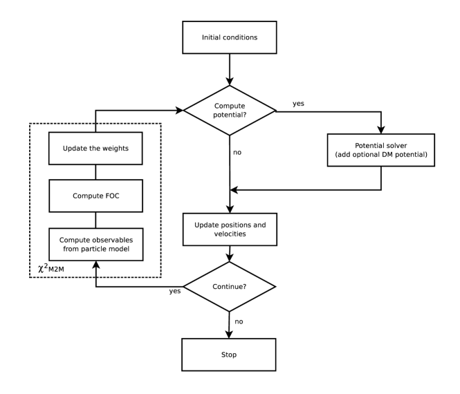
Figure 1: A high level flowchart describing NMAGIC. The main $\chi^{2}$M2M algorithm is contained in the dashed block, the remainder is an optional potential solver and code for moving the particles, both of which are exchangeable. In our tests, $\chi^{2}$M2M is generally applied only after a number of position/velocity updates.

The routine for updating the particle weights includes three main steps: First, all the observables used in the modeling process are computed as described above. Then we change the particle weights in accordance with equation (15) by

$$w_{i,t+\delta t}=w_{i,t}+\varepsilon w_{i,t}\left(\mu\frac{\partial S}{\partial w_{i}}-\sum_{j}\frac{K_{j}\left[{\mathbf{z}}_{i,t}\right]}{\sigma(Y_{j})}\widetilde{\mbox{{D}}}_{j,t}\right)\delta t,$$ (31)

with

$$\widetilde{\mbox{{D}}}_{j,t}=\frac{\widetilde{y}_{j,t}-Y_{j}}{\sigma(Y_{j})}.$$ (32)

Finally, we update the temporally smoothed observables as follows:

$$\widetilde{y}_{j,t+1}=\widetilde{y}_{j,t}+\alpha(y_{j,t}-\widetilde{y}_{j,t})\delta t.$$ (33)

Here $\delta t$ is the time between successive $\chi^{2}$M2M steps. All the differential equations here are ordinary differential equations of the form ${\mathrm{d}}y_{i}(t)/{\mathrm{d}}t=f_{i}(t,y_{1},\cdots,y_{N})$, and the $y_{i,n}$’s in our case are the particle weights $w_{i}$ or time-smoothed observables $y_{i}$ at $t_{n}$. We integrate them using a simple Euler method $y_{i,n+1}=y_{i,n}+h\;f(t_{n},y_{i,n})$ with $t_{n+1}=t_{n}+h$ and time step $h=\delta t$. We could replace the Euler method by the second-order Runge-Kutta method (cf. Press et al. 1992), which is more expensive and requires more memory. Since we are not interested in the details of how the weights converge, but only in the final converged system, a simple Euler method suffices for our purposes. We write $\varepsilon$ in equation (31) as $\varepsilon=\varepsilon^{\prime}\varepsilon^{\prime\prime}$ with $\varepsilon^{\prime\prime}=10/\max_{i,j}\{K_{ji}\,\widetilde{\mbox{{D}}}_{j}/\sigma(Y_{j})\}$. Thus $\varepsilon^{\prime\prime}$ times the last term in equation (15) is of order unity and we choose $2\varepsilon^{\prime}<\alpha$ to avoid excessive temporal smoothing.

The NMAGIC (N-particle Made-to-measure AlGorithm mInimizing Chi squared) correction routine can be combined with a standard $N$-body code including a potential solver and time integrator, or a fixed-potential routine and integrator when the target is to be modeled in a given gravitational potential. This last case is most similar to the Schwarzschild method. In most of the tests below, we use a fixed potential expanded in spherical harmonics.

However, in test E we allow the potential to vary, as we evolve from one triaxial model to another. For advancing the particles we use a standard leap frog time integrator with fixed time-step. The time-step value chosen leads to fluctuations of energy and angular momentum with amplitudes $5\times 10^{-6}$ and $2\times 10^{-5}$ around their initial values, without systematic drift, over 80 half mass dynamical times in the fixed potential case.

For test E, which models a triaxial system, a simple spherical harmonic expansion suffices for solving for the potential. We follow the method described by Sellwood (2003): we tabulate coefficients of a spherical harmonic expansion of the density on a 1-D radial grid but retain the exact angular dependence up to some adopted $l_{\rm max}$, the maximum order of the spherical harmonic expansion. We include terms up to $l_{\rm max}=4$ in this experiment. Particles are binned on the radial grid using the scheme described by Sellwood (2003). This then gives the forces on the grid, from which we interpolate back to a particle’s position for the gravitational forces. Test E involves a cuspy model; in order to properly resolve this we use a radial grid at radii $r_{\xi}=e^{\gamma\xi}-1$ with $\gamma=\ln(r_{\rm max}+1)/\xi_{\rm max}$; we use $\xi_{\rm max}=301$ for 301 shells and $r_{\rm max}=40$.

NMAGIC is written in Fortran 90 and parallelized with the MPI library. We distribute the $N$ particles as nearly evenly as possible over $N_{p}$ processors. Parallelizing in only the observables would not scale well with large $N_{p}$, because of the different nature of the observables, and would require a large memory on each processor when $N$ is large. In Figure 1 we present a high level flowchart of the operational logic of NMAGIC.

In order to test the scaling with $N_{p}$ of NMAGIC we considered $N=1.8\times 10^{6}$ and $N_{o}=816$ observables (640 density and 176 kinematic) with $N_{p}$ varying from 1 to 120. These values of $N_{p}$ and $N_{o}$ are adequate for the experiments presented here and are used in test C of Table 1. Since we are only interested in the scaling of the $\chi^{2}$M2M parallelization with $N_{p}$, we only execute the $\chi^{2}$M2M 50 times, without recomputing the potential or advancing particles. In Figure 2 we present these scaling results as time per step (left hand axis, plus symbols) and steps per unit time (right hand axis, open squares) as functions of $N_{p}$. We generally find that our implementation of $\chi^{2}$M2M scales very well with $N_{p}$. Defining the speedup $S(N_{p},N)$ as

$$S(N_{p},N)=\frac{T(1,N)}{T(N_{p},N)}$$ (34)

where $T(N_{p},N)$ is the time for computing $N$ particles on $N_{p}$ processors, we fit a standard Amdahl’s law (Amdahl, 1967)

$$S(N_{p},N)=\frac{1}{f+(1-f)/N_{p}},$$ (35)

in order to determine the fraction of sequential code, $f$. We obtained that $f\simeq 0.010$, i.e. the sequential part of the code accounts for only $1\%$.

Figure 2: The performance of our implementation of $\chi^{2}$M2M. We used $1.8\times 10^{6}$ particles without potential calculations or particle motion. On the left hand axis we label time per step required, with the corresponding data indicated by plus symbols, while on the right hand axis we label steps per unit time, with the corresponding data now shown by open squares. Note that the scale is logarithmic on the left and linear on the right. The fraction of sequential code, $f$, from these data was computed at $\sim 1\%$.

4 Target Models and Their Observables

We will test the NMAGIC code on spherical, axisymmetric, and triaxial target models. The spherical target is a particle model constructed from the analytic density and distribution function of an isotropic Hernquist sphere. As oblate target we take a maximally rotating three-integral model. Finally, we construct both a stationary and a rotating triaxial target system. We use the NMAGIC code itself to generate a dynamical equilibrium structure for these models. It will be seen that the $\chi^{2}$M2M method provides a very useful means to set up dynamical equilibrium models of galaxies for which no analytic distribution functions are known, in order to study the properties of such systems.

In the following subsections, we describe in turn each of these targets and their construction. We determine the target observables obtained from these models, and describe how we obtain errors for these observables. These will be needed in Section 5 where we present the results of building $\chi^{2}$M2M models to match these targets. The reader who is mainly interested in these tests of NMAGIC can in a first reading directly go to that section.

4.1 Spherical Target

Our first target is a spherical isotropic Hernquist (Hernquist, 1990) model, which we will refer to as target SIH. Its density and potential are given by

$$\varrho(r)=\frac{aM}{2\pi r(r+a)^{3}},\qquad\varphi(r)=-\frac{GM}{r+a},$$ (36)

where $a$ is the scale length, $M$ is the total mass, and $G$ is the gravitational constant. The projected effective (half-mass) radius equals $R_{\rm eff}\approx 1.8153a$. We use units such that $M=a=1$. The target mass $M_{k}$ on shell $r_{k}$ is given by the sum of the contributions of the adjacent shells,

$$M_{k}=4\pi\int\varrho(r)\gamma^{CIC}_{k}(r)r^{2}{\mathrm{d}}r.$$ (37)

The innermost (outermost) shell is an exception because only the layer immediately exterior (interior) contributes.

Figure 3: The mass in shells profile computed from equation (36) is shown as the solid line, whereas the dashed line illustrates the mass profile computed from a spherical Hernquist particle model generated from a truncated DF.

We construct SIH models on a radial grid with 40 shells, quasi-logarithmically spaced in radius with inner and outer boundaries at $r_{\rm min}=5\times 10^{-4}$ and $r_{\rm max}=20$. The distribution function is truncated at $E_{\rm max}\equiv\phi(r_{\rm max})$. At that truncation, the mass included is

$$M_{\rm trun}=\int_{E_{\rm min}=\varphi(0)}^{E_{\rm max}=\varphi(r_{\rm max})}\frac{dM}{dE}dE,$$ (38)

with $(dM/dE)$ the differential energy distribution (e.g. Binney & Tremaine 1987) and thus $M_{\rm trun}=0.86$. Figure 3 compares the mass on shells (hereafter “mass profile”) $M_{P}(r_{k})$ for a particle realization of this truncated distribution function (constructed using the method described in Debattista & Sellwood 2000), with the $M_{k}$ from the Hernquist density profile as in equation (37). For small radii the mass profiles match but for larger radii $M_{P}(r_{k})$ is significantly smaller than $M_{k}$ due to the finite extent of the particle realization, consisting only of particles with $E<E_{\rm max}=\varphi(r_{\rm max})$. Using $M_{k}$ as target observables would increase the mass of particles on the outer (near) circular orbits and would therefore increase the tangential velocity dispersion. We will thus use the $M_{P}(r_{k})$ as targets and omit the subscript $P$ in the following. We also include zero-valued higher order mass moments to enforce sphericity.

We assume Poisson errors for the radial mass: $\sigma(M_{j})=\sqrt{M_{j}M_{\rm trun}/N}$ where N is the total number of particles used in the particle model. For the errors in the higher order mass moments, we use Monte-Carlo experiments in which we generate particle realizations of the density field of the target model using $1.8\times 10^{6}$ particles, which is the same number as in the $\chi^{2}$M2M models.

Kinematics of the target can be computed from a DF. We use the isotropic DF (Hernquist 1990, Carollo et al. 1995)

$$f(E) \propto \frac{1}{(1-q^{2})^{5/2}}\big{(}3\arcsin(q)+q(1-q^{2})^{1/2}$$ (39)

$$\times(1-2q^{2})(8q^{4}-8q^{2}-3)\big{)}$$

with $q=\sqrt{-aE/GM}$, and $E$ is the energy. We determine kinematic observables of the target on a projected radial grid with 30 shells, quasi-logarithmically spaced in radius and bounded by $R_{\rm min}=0$ and $R_{\rm max}=10=5.51R_{\rm eff}$. On the shell midpoints we compute the $h_{2}$ and $h_{4}$ moments of the isotropic Hernquist model from the DF of equation (39). We will use integral field-like kinematic data to recover the spherical targets in Section 5. More precisely, we multiply the $h_{2,k}$ and $h_{4,k}$ moments by the projected mass of the truncated SIH model within each radial grid shell to obtain the mass-weighted higher order moments $M_{k}\,h_{2,k}$ and $M_{k}\,h_{4,k}$, which we use as the target observables. While this procedure is not perfectly self-consistent, because the moments are from the infinite extent analytic DF while the mass is from the truncated DF, the differences are very small. The main advantage of doing this is that it allows us to compute the uncertainties in these kinematic observables, which we assume $\sigma(M_{k}h_{n,k})=\sigma(h_{n})M_{c}\sqrt{M_{k}/M_{c}}$ with $\sigma(h_{n})=0.005$, $M_{k}$ the target mass in shell $k$, and $M_{c}$ the mass in the central grid shell.

4.2 An Oblate Three-Integral Target made with NMAGIC

Figure 4: The upper panel shows the mass profile computed from equation (40) for $q=0.6$ (solid line) and from a Hernquist particle model made from a DF and squeezed along the $z$-axis (dashed line). The lower panel is the same but for $A_{20}$.

Our oblate target model has density

$$\varrho(m)=\frac{aM}{2\pi qm(m+a)^{3}}$$ (40)

where $M$ and $a$ are total mass and scale radius, and $m^{2}=R^{2}+(z/q)^{2}$ with $q$ being the flattening. This density belongs to the family of flattened $\gamma$ models (Dehnen & Gerhard, 1994), with $\gamma=1$. We compute the gravitational potential from (cf. Binney & Tremaine 1987, section 2.3)

$$\varphi(R,z)=-\frac{GM}{2a}\int_{0}^{\infty}\frac{\tilde{\psi}(\tilde{m}){\mathrm{d}}\tau}{(1+\tau)\sqrt{\tau+q^{2}}}$$ (41)

with

$$\tilde{m}=\sqrt{\frac{R^{2}}{\tau+1}+\frac{z^{2}}{\tau+q^{2}}},$$ (42)

$$\tilde{\psi}(m)=1-\frac{m^{2}+2am}{(m+a)^{2}}.$$ (43)

by numerical integration, and tabulate it using a coarse and a fine linear grid in the meridional ($R-z$) plane. The coarse grid extends to $R=z=30a$ with $500\times 500$ grid points. To increase the resolution at small $R$ and $z$ we replace the $20\times 20$ “innermost” grid cells at $(R,z)=(0,0)$ to $(1.2a,1.2a)$ by a finer grid also consisting of $500\times 500$ grid points.

Figure 5: Kinematic major and minor axis slits for the oblate models, with the cells along each slit indicated. The ellipse corresponds to one $R_{\rm eff}$ of the equivalent Hernquist model squeezed by $0.6$ in the $z$ direction.

In our experiments, we view the model edge-on along the $x$-axis as line-of-sight. Our targets are the mass moments $A_{lm,k}$ of the three-dimensional density $\rho$, and – for these oblate models – the kinematic moments $m\;h_{n}$, $n=1,...,4$. We define an effective radius $R_{\rm eff}\approx 1.8153a$ which is equal to that of the spherical Hernquist model. We set $M=a=1$ and $q=0.6$. The target mass moments $A_{lm,k}$ on shell $r_{k}$ are given by the sum of the contributions of the adjacent shells and are computed through

$$A_{lm,k}=\int Y_{lm}(\theta,\phi)\varrho({\mathbf{x}})\gamma^{CIC}_{k}(r){\mathrm{d}}^{3}x.$$ (44)

The innermost (outermost) shell is an exception because only the layer immediately exterior (interior) contributes. The setup of the radial grid is identical to that used for the spherical model and for our tests below we use $M_{k}$, $A_{20,k}$, $A_{22,k}$, $\cdots$, $A_{66,k}$.

Figure 4 compares $M_{k}$ and $A_{20,k}$ computed from equation (40) with $M_{P}(r_{k})$ and $A_{P,20}(r_{k})$ obtained from a spherical Hernquist particle realization built from a DF and squeezed along the $z$-axis by $q=0.6$. As in Figure 3, $M_{P}(r_{k})$ and $A_{P,20}(r_{k})$ match $M_{k}$ and $A_{20,k}$ within $r\mathrel{\raise 2.0pt\hbox{\hbox to0.0pt{\hbox{\lower 6.0pt\hbox{$\sim$}}\hss}\hbox{$<$}}}5a$ but then approach zero at larger radii towards $r_{\rm max}$. This difference is again due to the finite extent of the particle model. Below we therefore use the radial mass profile $M_{P}$ and the higher mass moments $A_{P,lm}$ as targets, and again we omit the subscript $P$ in the following.

We assume errors in the target mass profile $\sigma(M_{j})$ as for the spherical model. For the errors in the higher order mass moments, we use Monte-Carlo experiments in which particle realizations of the density field of the target model are generated using $5\times 10^{5}$ particles, which is the same number as in the $\chi^{2}$M2M models.

In our oblate models we attempt to recover the target system from both slit and integral field kinematic data. Thus as kinematic target observables we use the projected mass-weighted Gauss-Hermite moments along the major and minor axes in Test C, and on a grid of $30\times 20$ points covering positions on the sky in $[-3.6,3.6]\times[-1.8,1.8]$ in Test D. A schematic representation of the slit setup is shown in Figure 5. The slits extend out to about $2R_{\rm eff}\simeq 3.6$.

The target kinematics are determined from a $4\times 10^{6}$ particle representation of a maximally rotating three-integral model for the density distribution of equation (40) with $q=0.6$. This is constructed by first evolving an isotropic spherical Hernquist model to the desired shape, using $\chi^{2}$M2M, and then switching the in-plane velocity vectors of all particles with positive angular momentum $J_{z}$ to negative $J_{z}$, leading to a DF which is still a valid solution of the Boltzmann equation (Lynden-Bell, 1960). For each slit or integral field cell $p$ we obtain the mass in that cell $M_{p}$ and the mass-weighted Gauss-Hermite moments $M_{p}\,h_{1,p},\cdots,\,M_{p}\,h_{4,p}$. We assume errors for the mass-weighted Gauss-Hermite coefficients as for the spherical model: $\sigma(M_{p}h_{n,p})=\sigma(h_{n})M_{c}\sqrt{M_{p}/M_{c}}$, where $M_{p}$ is the mass in slit cell $p$, computed by Monte-Carlo integration. In this case, we set $\sigma(h_{n})=0.005$ ($0.003)$ for the central slit (integral field grid) cell $m_{c}$ to approximate realistic errors.

4.3 Making Triaxial Models with NMAGIC

Figure 6: Target mass and $A_{20}$ profiles for the triaxial models. The solid line shows target T54 while the dashed line shows target T53.

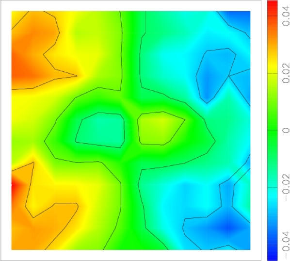
Figure 7: Line-of-sight velocity field of the rotating triaxial particle model (RT54K) as seen in the inertial frame. The co-rotation radius is $R_{\rm cor}\approx 10R_{\rm eff}$. The FoV extends from $-R_{\rm eff}$ to $R_{\rm eff}$ along each direction. Its lower edge is parallel to the major axis, the line-of-sight is parallel to the intermediate axis. Notice the counter-rotation near the center.

In the tests below we also explore triaxial Hernquist target models with stellar densities

$$\varrho(s)=\frac{Ma}{2\pi x_{0}z_{0}s(s+a)^{3}},$$ (45)

where $M$ is the total mass, $a$ the scale radius, and $s=\sqrt{(x/x_{0})^{2}+y^{2}+(z/z_{0})^{2}}$. Here $y$ is the longest axis, and the parameters $x_{0}$ and $z_{0}$ are the axis ratios. As before, we use units with $M=a=1$ and we define the effective radius with reference to the spherical model, i.e. $R_{\rm eff}\approx 1.815$. We generate two targets with different triaxialities, characterized by the triaxiality parameter $T=(1-x_{0}^{2})/(1-z_{0}^{2})$ (Franx et al., 1991). The more triaxial target, hereafter T53, has $x_{0}=0.9$ and $z_{0}=0.8$ ($T=0.53$) whereas the less triaxial target, hereafter T54, has $x_{0}=0.85$ and $z_{0}=0.7$ ($T=0.54$). In both cases the target is observed along its intermediate ($x$-)axis.

Like our oblate target model, the triaxial models cannot be represented by a DF based on the integrals of motion. We therefore construct them through particle realizations via a two step process. Starting from a spherical Hernquist particle realization made from a DF as before, we squeeze this along the x- and z-axes by factors $x_{0}$ and $z_{0}$, respectively, and compute the desired target density observables $M_{k}$ and the higher order mass moments $A_{20,k}$, $A_{22,k}$ up to $A_{60,k}$ using the same radial binning as in the spherical and oblate targets. $A_{lm}$ components with $l>6$ are small and we omit them. The squeezing is rigid, i.e. without regard to the internal motions. We repeat this 30 times, squeezing the spherical Hernquist model rigidly along random orientations to the desired shapes. From these 30 particle representations of the model we compute the means and one $\sigma$ variations around the mean for the $A_{lm,k}$. The former are taken as target density observables, the latter as their errors. The uncertainties on the radial mass in shells profile are taken to be $\sigma(M_{k})=\sqrt{M_{k}M_{\rm trun}/N}$ as before. Figure 6 shows the target mass and $A_{20}$ profiles as functions of radius for T54 (solid line) and T53 (dashed line) as well as their uncertainties.

After this first step, which only gives target density observables, we then use $\chi^{2}$M2M to evolve a spherical Hernquist model to generate self-consistent triaxial particle realizations of T54 and T53. In addition we generate a slowly tumbling version of T54 with corotation radius $R_{cor}\approx 10R_{\rm eff}$, by applying $\chi^{2}$M2M in the appropriately rotating frame. The final models now have self-consistent kinematics; in order to distinguish them from the purely density targets we refer to them as models T53K and T54K for the non-tumbling models and RT54K for the tumbling model.

These final self-consistent models T54K and RT54K can now be used as targets in their own right, and we can compute (observer frame) target kinematics $m_{p}h_{n,p}$ from them. We compute the kinematics of both T54K and RT54K on a $12\times 12$ grid extending from $-R_{\rm eff}$ to $R_{\rm eff}$. For the uncertainties in the kinematic observables we adopt $\sigma(m_{p}h_{n,p})=\sigma(h_{n})M_{c}\sqrt{M_{p}/M_{c}}$ with $\sigma(h_{n})=0.005$ the error in $h_{n}$, $M_{p}$ the mass in grid cell $p$, and $M_{c}$ the mass in the central grid cell. The $M_{p}$’s were obtained directly from the particles. The velocity field of the target system RT54K in the observer’s frame is shown in Figure 7. This velocity field is characterized by disk-like counter-rotation close to the mid-plane and near cylindrical rotation away from the plane. These kinematics for this slowly tumbling triaxial model represent a valid dynamical model, but are unlikely to be the unique dynamical solution for the model’s density distribution.

5 Tests of NMAGIC

In this section we will use the $\chi^{2}$M2M algorithm to solve some modeling problems of increasing dimensionality and complexity, starting with spherical systems and ending with rotating triaxial models. The goal of these experiments is to investigate the convergence of the code, the quality with which various data are modeled, and the degree to which known properties of the target models can be recovered from their simulated data. We will see how these issues depend on the initial model, geometry, and amount of data available.

Table 1 lists all the experiments that we have carried out, including the target and the initial model identifications. We will refer to the final $\chi^{2}$M2M models by the prefix ’F’ to the test model name (e.g., FA for the final model of Test A). Generally, these final models are obtained in two steps. First we use only the target density observables in the $\chi^{2}$M2M algorithm, and once these have converged, we add the kinematic observables. Finally, we integrate all orbits for some time in the potential without $\chi^{2}$M2M corrections to test whether equilibrium has been reached. Unless mentioned otherwise, we use $1.8\times 10^{6}$ particles and set the entropy parameter $\mu$ to a small ($\ll 1$) value; see the discussion in Section 5.1.1. In most experiments, the particle distribution is evolved in the fixed target potential (this is analogous to the Schwarzschild modelling approach), but we include one test (model E) in which we also let the gravitational potential evolve.

Test	ICs	Target	$\varepsilon^{\prime}$	$\varepsilon^{\prime\prime}$	$\mu$
A	RP	SIH	$0.025$	$6.32\;10^{-7}$	$4.3\;10^{-4}$
A2	RP	SIH	$0.025$	$1.32\;10^{-6}$	$4.3\;10^{2}$
A3	RP	SIH	$0.050$	$1.24\;10^{-6}$	$4.3\;10^{-4}$
A4	RP	SIH	$0.100$	$6.80\;10^{-7}$	$4.3\;10^{-4}$
B	SIH-2	SIH	$0.025$	$1.76\;10^{-6}$	$4.3\;10^{-4}$
C	ORIH	O3I	$0.05$	$3.94\;10^{-7}$	$0$
D	ORIH	O3I	$0.05$	$3.94\;10^{-7}$	$0$
E	T53K	T54K	$0.15$	$5.06\;10^{-8}$	$4.3\;10^{2}$
F	T54K	RT54K	$0.15$	$3.77\;10^{-8}$	$4.3\;10^{2}$

Table 1: Tests of NMAGIC carried out in this paper, with model names and parameters. For all models, we have used $\alpha=2.1\varepsilon^{\prime}$.

5.1 Spherical Models

5.1.1 Initial model and time-evolution

Figure 8: (a) Top: Time evolution of $\chi^{2}$ in test A. (b) Bottom: Time evolution of a set of 100 particle weights in test A. $w_{0}$ is the initial weight of the particles; $w_{0}=1/N$. The time-interval plotted includes a first phase of density adjustment ($t\leq 2250$), a second phase of density and kinematic adjustment ($2250<t\leq 4500$), and a final phase of free evolution during which the weights do not change ($t\geq 4500$). Time is in units where the dynamical time at the half-mass radius is 6.0, and the dynamical time at $r_{\rm max}$ is 150.

Figure 9: (a) Top: Radial mass and $A_{20}$ profiles for the target model SIH and the final models FA from Test A (solid line) and FB from Test B (dashed line). (b) Bottom: Kinematic profiles $m\,h_{2}$ and $m\,h_{4}$, for the same models. – In all panels, the data points with errors correspond to the SIH target, the solid line to the final particle model FA, and the dashed line to the final model FB. The error bars in the target mass distribution are not shown as they are smaller than the symbol sizes. The absolute errors shown decrease outwards due to the mass weighting; the corresponding relative errors increase outwards.

The aim of our first experiment, Test A, is to reproduce a spherical isotropic Hernquist (SIH) model by a $1.8\times 10^{6}$ particle model. We start by generating a Plummer model from its DF (e.g. Binney & Tremaine 1987), using the method described in Debattista & Sellwood (2000). The DF of the Plummer model is truncated at $\Phi(r_{\rm max})$, with $r_{\rm max}=20$, and has a scale length $b=1$ and unit total mass. We then relax these particles in the analytic Hernquist potential, which is held fixed while the particle orbits are integrated. We refer to the resulting particle distribution as initial model RP (relaxed Plummer).

Then with $\chi^{2}$M2M we first adjust the density distribution of model RP to that of the target SIH, using as target observables $M_{k}=\sqrt{4\pi}A_{00,k}^{t}$ (equation 37) and $A_{lm,k}^{t}=0$ for $1<l\leq 6$, $0<m\leq l$ (equation 23) with Monte Carlo errors estimated as described in Section 4.1. After convergence the even kinematic moment observables $M_{k}h_{2,k}$ and $M_{k}h_{4,k}$ are added with errors given also in Section 4.1. Finally the system is integrated for some time without applying the $\chi^{2}$M2M corrections.

The second experiment B is identical to A except that instead of model RP we use a second Hernquist model SIH-2 as initial conditions for NMAGIC. SIH-2 differs from the target model SIH in that its radial scale length $a=1.4$ instead of $a=1$.

Figure 8a shows the time evolution of $\chi^{2}/N_{o}$ of the particle model A during and after the $\chi^{2}$M2M evolution. Throughout $N_{o}$ refers to all the observables, density and kinematics, regardless of whether they are being used in the FOC or not; thus $N_{o}$ is a constant. The time evolution of a sample of 100 particle weights of the SIH particle model is presented in Figure 8b. From these figures one sees that the overall $\chi^{2}/N_{o}$ decreases quickly at the beginning of both phases (density adjustment only phase, and a density and kinematic observable adjustment phase). However, particle weights keep evolving for significantly longer time-scales. For this reason we integrate and adjust particle weights in both phases for relatively long times, about 15 dynamical times at $r_{\rm max}$.

5.1.2 Convergence to the target observables for different initial conditions

Figure 10: Histogram of the particle weights in the final FA model, obtained from Plummer model initial conditions (solid line). The dashed line shows the histogram of particle weights when spherical Hernquist ICs with scale length $a=1.4$ were used (FB). $w_{0}$ is the initial weight of the particles; $w_{0}=1/N$ in all cases.

The fit of the final particle models FA and FB to the observables is illustrated in Figure 9. The top panel shows the radial mass and $A_{20}$ coefficient, whereas the bottom panel shows the kinematic targets and final model observables for $m\,h_{2}$ in the upper and $m\,h_{4}$ in the lower panel. As can also be seen from Fig. 8, the final model fits the input data to within $1\sigma$. The corresponding error bars are smaller than the crosses in the top panel of Fig. 9; see Fig. 6 for an example. The same is true for $A_{20}$ except when the target values are zero as in Fig. 9. Error bars for the mass observables are therefore not plotted in this and subsequent similar figures.

All model observables in Fig. 9 are temporally smoothed observables as in equation (19). After some free evolution with $\chi^{2}$M2M turned off both models fit the target data within the errors. The free evolution is necessary because $\chi^{2}$M2M pushes the model towards a perfect fit to the observables, at the expense of continually changing particle weights. Deviations are largest in the outer parts where orbital time-scales are longest. Model FB, which had an initial particle distribution closer to the target, is generally smoother and fits the data better, but differences are within the errors. NMAGIC achieved satisfactory models even from the less favorable, cored Plummer initial conditions.

Figure 10 compares the histogram of final particle weights of the FA and FB models, all normalized by their initial weight. Model FA has a significant tail towards high weights, and a peak at correspondingly lower particle weight such that the mean particle weight is the same as for the more symmetric weight distribution of model FB. On average, the weights of particles in model FA had to change by more than those in model FB. We can quantify this by defining an effective particle number $N_{\rm eff}$ characterizing mass fluctuations through

$$N_{\rm eff}\equiv N{\overline{w}^{2}\over\overline{w^{2}}},$$ (46)

where $\overline{w}$ and $\overline{w^{2}}$ are the mean and mean-square particle weights. This reduces to $N$ for equal-mass particles, to one when one particle dominates, and discards particles with near-zero weights. For the final models FA and FB the effective numbers of particles are $N_{\rm eff}=5.7\times 10^{5}$ and $1.5\times 10^{6}$, respectively, while for both models $N=1.8\times 10^{6}$.

Figure 11: (a) Top: Radial density profiles in the spherical models. Uppermost panel: Density profiles for the Hernquist target profile, SIH (stars), the final models FA (dashed line) and FB (dash-dotted line), and their respective initial condition models RP and SIH-2 (dotted and dash-triple-dotted lines). Middle panel: Relative deviation from the target density $\mbox{{D}}\rho/\rho$, for the two models FA and FB using the same line styles. (b) Bottom: Differential energy distributions. The truncated analytic Hernquist DF used for target SIH is shown by the star symbols. The dashed line corresponds to the final $\chi^{2}$M2M model FA, and the dotted line indicates the relaxed Plummer initial conditions RP.

The origin of this difference between the two models can be seen from Figure 11a, which plots the radial density profile of the target SIH (stars), the initial models RP and SIH-2, and the temporally smoothed final models. We computed the densities using the identical radial grid as was used for the mass targets. The density profile of the SIH target is well reproduced by the final particle models FA and FB across more than a factor of 100 in radius. The largest relative deviation in the density $\delta\rho/\rho$ occurs at small radii and never reaches more than $5\%$. In this region, model RP has few particles and the large relative error is due to Poisson noise. Model FB, which starts out closer to the target SIH fits better in this region.

Model RP is clearly significantly less dense than SIH inside $r\simeq 0.3a$; it has a core whereas the target profile is cuspy. Also, it has a steeper outer density profile than the target model. To match model RP to SIH therefore requires NMAGIC to increase the particle masses both in the central regions and in the outer halo of the model. This causes the high-weight tail in the distribution in Fig. 10, as we verified by inspecting the positions of particles with $w_{i}>2w_{0}$.

Figure 11b presents the differential energy distributions. The final particle model FA matches the analytic differential energy distribution of the isotropic Hernquist model (equation 39) very well.

Figure 12: (a) (b) Top: Internal kinematics of the final model FA. The upper panel show $\sigma_{r}$, $\sigma_{\varphi}$ and $\sigma_{\theta}$, the lower panel the $v_{r}$, $v_{\varphi}$ and $v_{\theta}$. The stars correspond to the analytic $\sigma_{r}$ from the untruncated DF. Model FA is very nearly isotropic and has negligible rotation, despite starting from anisotropic initial conditions. Bottom: Anisotropic internal kinematics of the initial model RP. The dotted, dashed, and dash-dotted lines show $\sigma_{r}$, $\sigma_{\varphi}$, and $\sigma_{\theta}$ of the RP particle model. For comparison, the solid line corresponds to the analytic $\sigma_{r}$ of the untruncated analytic DF of the SIH target model.

As a final test, Figure 12a shows the intrinsic velocities (lower panel) and velocity dispersions (upper panel) of the analytic, untruncated DF and the final $\chi^{2}$M2M model FA. The match to the target kinematics is good and model FA is nearly isotropic, despite the fact that it has evolved from an initial RP model that is moderately anisotropic. The anisotropy of the initial model RP is shown in Figure 12b which compares its intrinsic velocity dispersions $\sigma_{r}$, $\sigma_{\varphi}$ and $\sigma_{\theta}$ with the analytic $\sigma_{r}$ of the SIH target model. The residual anisotropy in model FA is caused by the relative absence of radial orbits resulting from truncating the DF.

5.1.3 Dependence on $\epsilon^{\prime}$ and $\mu$

Figure 13: (a) Top: Radial density profiles for various spherical models constructed for the Hernquist target profile, SIH. Upper panel: Density profiles for the target model (stars), the model FA (dashed line) and several tests that differ from model FA by the values of the parameters $\varepsilon^{\prime}$ and $\mu$ (see Table 1). Middle panel: Relative deviation from the target density $\mbox{{D}}\rho/\rho$, for the same models. (b) Bottom: Differential energy distributions. Stars: target model SIH. Lines: same models as in top panel.

Figure 14: Histogram of the particle weights in the final FA model, obtained from Plummer model initial conditions (solid line). The other histograms show the particle weight distributions for models FA2 (dashed), FA3(dash-dotted), and FA4 (dotted). $w_{0}$ is the initial weight of the particles; $w_{0}=1/N$ in all cases.

In the tests described so far, we have used $\epsilon^{\prime}=0.025$ for the correction steps in the FOC. In general, small values of $\epsilon^{\prime}$ result in a smooth evolution but slow convergence, whereas large values of $\epsilon^{\prime}$ change the global model too rapidly to attain a properly phase-mixed stationary solution. Thus generally we have found $\epsilon^{\prime}\mathrel{\raise 2.0pt\hbox{\hbox to0.0pt{\hbox{\lower 6.0pt\hbox{$\sim$}}\hss}\hbox{$<$}}}0.1$ to give good results. This is illustrated in Fig. 13, which shows that test A converges to essentially identical density distributions and differential energy distributions for values of $0.025\leq\epsilon^{\prime}\leq 0.1$ (models FA, FA3, FA4). Only for the largest value $\epsilon^{\prime}=0.1$ do we start seeing small deviations in the density profile of more than a few percent from the target model. Also, the effective particle number [equation (46)] decreases from $5.7\times 10^{5}$ through $3.3\times 10^{5}$ to $1.0\times 10^{5}$ for models FA, FA3, and FA4, respectively. Thus we will generally use $\epsilon^{\prime}<0.1$, but because the speed of convergence also depends on the number and kind of observables used for the corrections, we have sometimes also increased $\epsilon^{\prime}$ slightly. Figure 14 shows the distributions of particle weights for these models. They develop larger wings for larger values of $\epsilon^{\prime}$. Because particles weights are then changed by larger amounts, the reshuffling is greater until convergence is reached.

In models FA and FB, we have also set the entropy parameter $\mu$ to a small ($\ll 1$) value, which allows the NMAGIC code to concentrate on fitting the data. (Note that, because the term $K_{ij}\,\widetilde{\mbox{{D}}}_{j}/\sigma(Y_{j})$ in the FOC is large, even $\mu=1.0$ leads to only a small contribution of the entropy terms in the FOC). While the purpose of not setting $\mu$ to zero exactly originally was to prevent overly large fluctuations in the particle weights, in fact, a test with $\mu=0$ has given essentially identical results to the ones reported. Fig. 13 shows that also for model FA2 with $10^{6}$ times larger entropy parameter than in model FA, the target density and differential energy distribution are fitted equally well as before. Generally, the best value to use for the entropy depends on the initial model, the data to be fitted, and the intrinsic structure of the target, and it must be determined separately for each application. A more systematic investigation of the effect of the entropy term is therefore deferred to a future paper in which we will use $\chi^{2}$M2M to model and determine mass-to-light ratio, anisotropy, etc., for a real galaxy.

5.2 Oblate Models

The task we set the algorithm here is a difficult one: starting from a non-rotating system, we see whether we can recover the maximally rotating three-integral model described in Section 4.2, in which the weights of all counter-rotating particles should be zero. We perform two such experiments, one using slit data as kinematic targets (Test C), the second using integral field kinematic targets (Test D). As in the spherical experiments, we keep the potential fixed while evolving the system with $\chi^{2}$M2M in runs C and D.

Both experiments start from an initial model which is constructed by relaxing a spherical Hernquist particle model consisting of $5\times 10^{5}$ particles in the oblate potential. As in experiments A and B, we then apply $\chi^{2}$M2M in 2 steps, first for the density alone, and when this has converged, for both the density and kinematics. The density part of the runs is identical for experiments C and D.

Figure 15: The mass and mass $A_{20}$ profiles for the oblate models. The data points show the target and the lines shows the converged models FC (dashed) and FD (full).

Figure 16: Mass-weighted higher order moments along the major and minor axes for the slit-reconstructed oblate model FC. The target observables are shown as error bars, whereas the model observables for model FC are indicated by the dashed lines, respectively. Kinematics along the major axis are shown on the left and those along the minor axis on the right.

Figure 17: Gaussian best fit velocity (top left), velocity dispersion (top right), Gauss-Hermite moments $h_{3}$ (bottom left) and $h_{4}$ (bottom right) along the major axis (left) and minor axis (right), for the models with slit data targets (dashed line), integral field kinematic targets (full), and the initial model (dotted). The error bars show the target kinematics.

Figure 18: Distribution of particle weights in the final models FC (top) and FD (bottom).

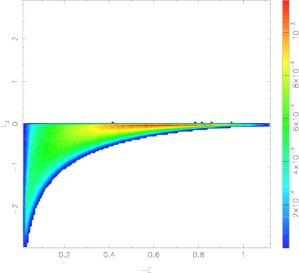
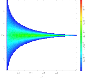
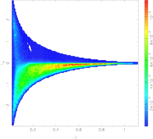
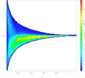
Figure 19: Particle weight distributions projected onto the ($E,L_{z}$) plane, for the maximally rotating three-integral target (top left), the initial relaxed isotropic Hernquist model (top right), and the two models reconstructed from density and slit kinematic targets (FC, bottom right) and from density and integral field kinematics (bottom left).

Figure 15 plots the mass and $A_{20}$ radial profiles of the target (error bars) and the final $\chi^{2}$M2M models FC and FD. As in the spherical tests, the target density distribution is very well fitted by the $\chi^{2}$M2M models.

The mass-weighted kinematics along the major and minor axes of model FC are shown in Figure 16, while Figure 17 show the as-observed kinematics of both models. The latter are calculated by dividing the mass-weighted moments by the mass in the slit resp. grid cell, and using the relations $v=v_{\rm targ}-\sqrt{2}\sigma_{\rm targ}h_{1}$ and $\sigma=\sigma_{\rm targ}-\sqrt{2}\sigma_{\rm targ}h_{2}$ (e.g. , Rix et al. 1997). All kinematic quantities for the reconstructed models are shown $\Delta t=500$ ($\mathrel{\raise 2.0pt\hbox{\hbox to0.0pt{\hbox{\lower 6.0pt\hbox{$\sim$}}\hss}\hbox{$>$}}}3$ dynamical times at $r_{\rm max}$) after switching off the $\chi^{2}$M2M corrections. The fits are generally excellent except for the higher order moments near the boundaries of the kinematic fit regions, where counter-rotating particles with high energies still make significant contributions, because their weights have not yet been sufficiently reduced.

Figure 18 showing the weight distributions for both models FC and FD clearly illustrates the stronger constraints placed on the model by the integral field data. In both models, the NMAGIC code works at reducing the weights of the counter-rotating particles, but has clearly gone a lot further in model FD.

Finally, in Figure 19 we show the distribution of weights in the ($E,L_{z}$) plane for the target model, initial relaxed model, and the two models FC and FD. The success of the $\chi^{2}$M2M method in removing the counter-rotating particles amply present in the initial model is apparent, particularly for model FD. Of course, in applications aimed at obtaining a best-fit representation of some galaxy kinematic data it would have been smart to start the iterations from an initial model that is better adapted to the problem at hand.

5.3 Triaxial Models

5.3.1 Evolving the potential self-consistently

We illustrate NMAGIC’s capabilities with two very different triaxial model experiments. In run E, we start with the self-consistent model T53K as initial conditions and use NMAGIC to converge to target T54K. With this model, we test the full capabilities of $\chi^{2}$M2M, which make this technique more general than Schwarzschild’s method: in model E, we solve for the potential as the system evolves and follow the model in its self-consistent potential throughout, akin to an $N$-body experiment. For this purpose we use the spherical harmonic potential solver described in Section 3 above and update the potential after every 25 $\chi^{2}$M2M steps.

The resulting final model FE gives an excellent match to the density of the target model T54K, as is apparent from comparing the $M_{k}$ and $A_{20}$ profiles in Figure 20. Figure 21 shows the kinematics within $R_{\rm eff}$ of the models T54K and FE. All mass-weighted kinematic observables $m\,h_{1}$,…, $m\,h_{4}$ of the final model match the target observables at better than one $\sigma$ over almost the entire FoV, except for a few isolated regions reaching two $\sigma$. The random location of these deviations imply that they are due only to Poisson noise in the target model, the observables of which have not been temporally smoothed.

Figure 20: Mass and $A_{20}$ profiles for experiment E. The dots show the target T54K and the solid lines show FE.

Figure 21: The difference between kinematics in model T54K and model FE. The observables of FE are the temporally smoothed mass-weighted moments while those of T54K are not temporally smoothed. The differences have been divided by the corresponding assumed errors. The FoV extends from $-R_{\rm eff}$ to $R_{\rm eff}$ along each direction.

5.3.2 Rotating vs. non-rotating models

Test F is an interesting experiment in different ways. Starting from T54K, we use NMAGIC to attempt to converge to the observables of the tumbling target model RT54K, with a triaxial model which does not tumble but remains stationary relative to the observer. Thus this experiment explores whether it is possible to identify a kinematic signature of slow figure rotation in elliptical galaxies. Since the initial conditions possess neither rotation nor internal net stellar streaming, if this model fails to converge it may well be because the problem admits no solution. Because of this, test F is interesting in its own right, apart from as a validation of NMAGIC.

In fact, NMAGIC was able to converge the mass-weighted kinematic moments to within about one $\sigma$ of their target values; however, the residuals maps (Figure 22) show spatially correlated residuals in $mh_{1}$. When we compare the global velocity field of model FF with that of RT54K we find that the degree of cylindrical rotation around the tumbling axis ($z$-axis) is higher in RT54K than it is in model FF (Figure 23). Near the mid-plane, instead, the velocity field of both models is very similar, including the counter-rotation seen near the center. We can explore whether the residual differences are due to having assumed too large errors in the mass-weighted moments by decreasing the errors by a factor of five. The corresponding final model looks very similar to model FF but now with reduced $\chi^{2}>4$. Thus the difference is likely intrinsic and can be used to recognize a tumbling galaxy. A more complete analysis of this problem will be undertaken elsewhere (De Lorenzi et al. in progress).

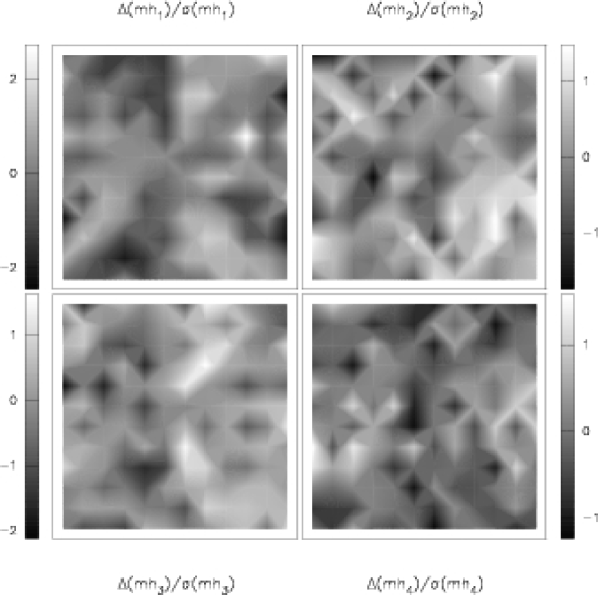
Figure 22: The difference between kinematics in target RT54K and model FF. The observables are the mass-weighted higher order moments, and have been divided by the corresponding assumed errors. The kinematics of RT54K are instantaneous but those of FF are time-averaged. The FoV extends from $-R_{\rm eff}$ to $R_{\rm eff}$ along each direction.

Figure 23: Left: Line-of-sight velocity field of the final non-tumbling triaxial particle model FF. Right: Difference of the line-of-sight velocity fields between the non-tumbling triaxial particle model FF and the tumbling target galaxy RT54K divided by the errors as described in the text. We assume an error in the mean velocity $\sigma(v_{j})=\sqrt{2}\sigma(h_{1})\sqrt{m_{c}/m_{j}}\sigma_{j}$, where we assumed $\sigma(h_{1})=-\sqrt{1/2}\sigma(v)/\sigma$ (Rix et al., 1997). In both panels the FoV extends from $-R_{\rm eff}$ to $R_{\rm eff}$ along each direction.

6 Conclusions

We have presented a made-to-measure algorithm for constructing particle models of stellar systems from observational data, building on the made-to-measure method of Syer & Tremaine (1996, ST96). An important element of our new method is the use of the standard $\chi^{2}$ merit function at the heart of the algorithm, in place of the relative error used by ST96. The improved algorithm, which we label $\chi^{2}$M2M, allows us to assess the quality of a model for a set of target data directly, using a statistically well-defined quantity ($\chi^{2}$). Moreover, this quantity is well-defined and finite also when a target observable takes on zero values.

This property has enabled us to incorporate kinematic observables including higher-order Gauss-Hermite moments into the force-of-change equation. Kinematic and density (or surface density) observables can then be used simultaneously to correct the particle weights. The price of changing to $\chi^{2}$M2M from the original formulation is that the kernels which project the particle weights and phase-space coordinates into model observables cannot themselves depend on the particle weights. In general this is quite natural for (volume or surface) density observables. For the kinematics this means that we need to use mass-weighted kinematic observables. Nonetheless, this is not a significant limitation.

We have implemented the $\chi^{2}$M2M method in a fast, parallel code, NMAGIC. This code also incorporates an optional but fast potential solver, allowing the potential to vary along with the model density. Its implementation of the $\chi^{2}$M2M algorithm is highly efficient, with a sequential fraction of only $\sim 1\%$. This has allowed us to build various models with large numbers of particles and based on many observables, and to run them for $\sim 10^{6}$ steps.

Then we have carried out a number of tests to illustrate the capabilities and performance of NMAGIC, employing spherical, oblate and triaxial target models. The geometric flexibility by itself is one of the main strengths of the method – no symmetry assumptions need to be made.

In the spherical experiments NMAGIC converged to the correct isotropic model from anisotropic initial conditions, demonstrating that a unique solution, if present, can be recovered. Both the truncated distribution function and the intrinsic velocity dispersions were recovered correctly. Two initial models with different density distributions were used in these experiments. While both converged to the final isotropic model, that with density closer to the density of the final model had smaller final deviations from the target observables, and a narrower distribution of weights. In both experiments, the observables (density and integral field-like kinematics) each converged in a few dynamical times at the outer boundary $t_{d,o}$, whereas the particle weights kept evolving for significantly longer, $\sim 10t_{d,o}$.

In the oblate experiments we gave the algorithm a difficult problem to solve. The target system was a maximally rotating three-integral model in which the weights of all counter-rotating particles were zero. Using density observables and either slit or integral field kinematics, NMAGIC was asked to recover this maximally rotating model starting from an isotropic spherical system relaxed in the oblate potential. After about 100’000 correction steps, particle weights on the counter-rotating side were reduced by a factor of $\sim 50$, the distribution of weights approached that of the target, and a good fit to the kinematic constraint data was achieved. Only near the boundary of the kinematic data did particles on orbits further out, whose weights had not yet converged, still cause some deviations from the target kinematics. These experiments also clearly showed the advantage of integral field data over slit data for constraining the model.

Our triaxial experiments showed that it is possible to start from one triaxial model and converge to another. We anticipate that this ability will be very useful in constructing models for the triaxial elliptical galaxies with which nature confronts us. One of these triaxial experiments included a potential update step every 25 $\chi^{2}$M2M steps, demonstrating that including an evolving potential is also practical.

In the final experiment, we first generated a particle model of a slowly tumbling triaxial system to use as a target. We then matched its volume density and line-of-sight kinematics with a stationary model. We showed that the mass-weighted kinematic moments of the figure rotating system was fitted to within one $\sigma$ by the non-rotating system out to $R_{\rm eff}$. However the residuals in the first order kinematic moment are correlated, which gives a clear signature of tumbling which the non-tumbling model is not able to match, even when the assumed errors are decreased by a significant factor. We thus conclude that, at least for this triaxial system, it is possible to distinguish between internal stellar streaming and pattern rotation within $R_{\rm eff}$ provided a full velocity field is available. A more complete study of this problem will be presented elsewhere.

This experiment also demonstrates the usefulness of the $\chi^{2}$M2M algorithm for modeling mock (rather than real) galaxies in order to learn about their dynamics. We note that such an experiment would not have been practical with standard $N$-body simulations.

Compared to the Schwarzschild method, the main advantages of the $\chi^{2}$M2M algorithm as implemented in NMAGIC are that (i) stellar systems without symmetry restrictions can be handled relatively easily, (ii) it avoids complicated procedures for sampling, binning, and storing orbits, and (iii) the potential can be evolved self-consistently if needed. In the examples given, a simple isotropic spherical model was evolved into a suitable initial model, which contained the required wide range of orbital shapes. Every $\chi^{2}$M2M model corresponds to a new set-up of a complete orbit library in the Schwarzschild method; so in problems where the same orbit library can be reused, Schwarzschild’s method will be faster. However, NMAGIC is highly parallel, so suites of models with $\sim 10^{6}$ particles are feasible on a PC cluster.

There is clearly room for improving the current implementation of the $\chi^{2}$M2M algorithm, and there is a need to study carefully the parameters that enter the algorithm, such as magnitude and frequency of the correction steps, entropy, etc., which we will address in future work.

However, the different applications presented in this paper show that the $\chi^{2}$M2M algorithm is practical, reliable and can be applied to various dynamically relaxed systems. High quality dynamical models of galaxies can be achieved which match targets to $\sim 1\sigma$ for plausible uncertainties in the observables, and without symmetry restrictions. We conclude that $\chi^{2}$M2M holds great promise for unraveling the nature of galaxies.

References

- Amdahl (1967) Amdahl, G. M. 1967, in AFIPS Conference Proceedings vol. 30 (Atlantic City, N.J., Apr. 18-20). AFIPS Press, Reston, Va., 483–+
- Binney & Tremaine (1987) Binney, J., & Tremaine, S. 1987, Galactic Dynamics (Princeton, NJ, Princeton University Press)
- Bishop (1987) Bishop, J. L. 1987, ApJ, 322, 618
- Bissantz et al. (2004) Bissantz, N., Debattista, V. P., & Gerhard, O. 2004, ApJ, 601, L155
- Cappellari et al. (2002) Cappellari, M., Verolme, E. K., van der Marel, R. P., Kleijn, G. A. V., Illingworth, G. D., Franx, M., Carollo, C. M., & de Zeeuw, P. T. 2002, ApJ, 578, 787
- Carollo et al. (1995) Carollo, C. M., de Zeeuw, P. T., & van der Marel, R. P. 1995, MNRAS, 276, 1131
- Copin et al. (2004) Copin, Y., Cretton, N., & Emsellem, E. 2004, A&A, 415, 889
- Cretton et al. (1999) Cretton, N., de Zeeuw, P. T., van der Marel, R. P., & Rix, H.-W. 1999, ApJS, 124, 383
- Debattista & Sellwood (2000) Debattista, V. P., & Sellwood, J. A. 2000, ApJ, 543, 704
- Dehnen & Gerhard (1993) Dehnen, W., & Gerhard, O. E. 1993, MNRAS, 261, 311
- Dehnen & Gerhard (1994) —. 1994, MNRAS, 268, 1019
- Dejonghe (1984) Dejonghe, H. 1984, A&A, 133, 225
- Dejonghe (1986) —. 1986, Physics Reports, 133, 217
- Dejonghe & de Zeeuw (1988) Dejonghe, H., & de Zeeuw, T. 1988, ApJ, 333, 90
- Franx et al. (1991) Franx, M., Illingworth, G., & de Zeeuw, T. 1991, ApJ, 383, 112
- Gebhardt et al. (2003) Gebhardt, K., Richstone, D., Tremaine, S., Lauer, T. R., Bender, R., Bower, G., Dressler, A., Faber, S. M., Filippenko, A. V., Green, R., Grillmair, C., Ho, L. C., Kormendy, J., Magorrian, J., & Pinkney, J. 2003, ApJ, 583, 92
- Gerhard (1991) Gerhard, O. E. 1991, MNRAS, 250, 812
- Gerhard (1993) —. 1993, MNRAS, 265, 213
- Hernquist (1990) Hernquist, L. 1990, ApJ, 356, 359
- Hunter & de Zeeuw (1992) Hunter, C., & de Zeeuw, P. T. 1992, ApJ, 389, 79
- Hunter & Qian (1993) Hunter, C., & Qian, E. 1993, MNRAS, 262, 401
- Kronawitter et al. (2000) Kronawitter, A., Saglia, R. P., Gerhard, O., & Bender, R. 2000, A&AS, 144, 53
- Kuijken (1995) Kuijken, K. 1995, ApJ, 446, 194
- Lucy (1974) Lucy, L. B. 1974, AJ, 79, 745
- Lynden-Bell (1960) Lynden-Bell, D. 1960, MNRAS, 120, 204
- Magorrian (1995) Magorrian, J. 1995, MNRAS, 277, 1185
- Matthias & Gerhard (1999) Matthias, M., & Gerhard, O. 1999, MNRAS, 310, 879
- Merritt (1996) Merritt, D. 1996, AJ, 112, 1085
- Ollongren (1962) Ollongren, A. 1962, Bull. Astron. Inst. Neth., 16, 241
- Press et al. (1992) Press, W. H., Teukolsky, S. A., Vetterling, W. T., & Flannery, B. P. 1992, Numerical recipes in FORTRAN. The art of scientific computing (Cambridge: University Press, —c1992, 2nd ed.)
- Qian et al. (1995) Qian, E. E., de Zeeuw, P. T., van der Marel, R. P., & Hunter, C. 1995, MNRAS, 274, 602
- Rix et al. (1997) Rix, H.-W., de Zeeuw, P. T., Cretton, N., van der Marel, R. P., & Carollo, C. M. 1997, ApJ, 488, 702
- Romanowsky & Kochanek (2001) Romanowsky, A. J., & Kochanek, C. S. 2001, ApJ, 553, 722
- Saaf (1968) Saaf, A. F. 1968, ApJ, 154, 483
- Schwarzschild (1979) Schwarzschild, M. 1979, ApJ, 232, 236
- Sellwood (2003) Sellwood, J. A. 2003, ApJ, 587, 638
- Syer & Tremaine (1996) Syer, D., & Tremaine, S. 1996, MNRAS, 282, 223
- Thomas et al. (2005) Thomas, J., Saglia, R. P., Bender, R., Thomas, D., Gebhardt, K., Magorrian, J., Corsini, E. M., & Wegner, G. 2005, MNRAS, 360, 1355
- Valluri et al. (2004) Valluri, M., Merritt, D., & Emsellem, E. 2004, ApJ, 602, 66
- van de Ven et al. (2003) van de Ven, G., Hunter, C., Verolme, E. K., & de Zeeuw, P. T. 2003, MNRAS, 342, 1056
- van der Marel & Franx (1993) van der Marel, R. P., & Franx, M. 1993, ApJ, 407, 525
- Verolme et al. (2002) Verolme, E. K., Cappellari, M., Copin, Y., van der Marel, R. P., Bacon, R., Bureau, M., Davies, R. L., Miller, B. M., & de Zeeuw, P. T. 2002, MNRAS, 335, 517