Constraining supernova models using the hot gas in clusters of galaxies

Abstract

Context. The hot X-ray emitting gas in clusters of galaxies is a very large repository of metals produced by supernovae. During the evolution of clusters, billions of supernovae eject their material into this Intra-Cluster Medium (ICM).

Aims. We aim to accurately measure the abundances in the ICM of many clusters and compare these data with metal yields produced by supernovae. With accurate abundances determined using this cluster sample we will be able to constrain supernova explosion mechanisms.

Methods. Using the data archive of the XMM-Newton X-ray observatory, we compile a sample of 22 clusters. We fit spectra extracted from the core regions and determine the abundances of silicon, sulfur, argon, calcium, iron, and nickel. The abundances from the spectral fits are subsequently fitted to supernova yields determined from several supernova type Ia and core-collapse supernova models.

Results. We find that the argon and calcium abundances cannot be fitted with currently favoured supernova type Ia models. We obtain a major improvement of the fit, when we use an empirically modified delayed-detonation model that is calibrated on the Tycho supernova remnant. The two modified parameters are the density where the sound wave in the supernova turns into a shock and the ratio of the specific internal energies of ions and electrons at the shock. Our fits also suggest that the core-collapse supernovae that contributed to the enrichment of the ICM had progenitors which were already enriched.

Conclusions. The Ar/Ca ratio in clusters is a good touchstone for determining the quality of type Ia models. The core-collapse contribution, which is about 50% and not strongly dependent on the IMF or progenitor metallicity, does not have a significant impact on the Ar/Ca ratio. The number ratio between supernova type Ia and core-collapse supernovae suggests that binary systems in the appropriate mass range are very efficient ($\sim$ 5–16%) in eventually forming supernova type Ia explosions.

1 Introduction

Clusters of galaxies are the largest gravitationally bound objects in the universe. About 80% of the baryonic matter in the clusters is in the form of hot X-ray emitting gas that has been continuously enriched with metals since the first massive stars exploded as supernovae. The abundances of elements in this hot Intra-Cluster Medium (ICM) therefore correspond to the time-integrated yield of the supernova products that reached the ICM. About 20–30% of the supernova products is being locked up in stars in the member galaxies (Loewenstein 2004). Because of the huge mass of the accumulated metals in the ICM, clusters of galaxies provide a unique way to test nucleosynthesis models of supernovae on a universal scale.

Since the launch of the ASCA satellite, it has been possible to do abundance studies using multiple elements. Several groups (e.g. Finoguenov et al. 2000; Fukazawa et al. 2000; Finoguenov et al. 2001; Baumgartner et al. 2005) used ASCA observations of a sample of clusters to study the enrichment of the ICM. They were able to measure the abundances of iron, silicon, and sulfur. Also neon, argon, and calcium were sometimes detected, but with relatively low accuracy. The spatial distributions of iron and silicon indicated that the core of the clusters is dominated by SN Ia products (Fe), while the outer parts of the clusters appear to be dominated by core-collapse supernova products (O). Using ASCA observations some authors already tried to constrain the specific flavour of supernova type Ia models (e.g. Dupke & Arnaud 2001). Others, like Baumgartner et al. (2005) used ASCA data to find that Population-III stars should play an important role in the enrichment of the ICM. However, this result is debated (de Plaa et al. 2006).

With the XMM-Newton observatory (Jansen et al. 2001), which has both a better spectral resolution and a much larger effective area compared to ASCA, it is in principle possible to extend the number of detectable elements to nine. The first abundances determined from a sample of clusters observed with XMM-Newton were published by Tamura et al. (2004). The general picture from the ASCA samples was confirmed, except for the fact that the silicon and sulfur abundance show a centrally-peaked spatial profile like iron. The oxygen abundance appears to be more uniformly distributed in the clusters.

Recently, Werner et al. (2006) and de Plaa et al. (2006) analysed deep XMM-Newton observations of the clusters 2A 0335+096 and Sérsic 159-03, respectively. They were able to accurately measure the global abundances of about nine elements in the cluster and fit them using nucleosynthesis models for supernovae type Ia and core-collapse supernovae. The fits show that $\sim$30% of all the supernovae in the cluster are type Ia and about 70% are core-collapse supernovae. In their data, they found a clear hint that the calcium abundance in these clusters is higher than expected.

In this paper, we extend the approach of de Plaa et al. (2006) and Werner et al. (2006) to a sample of 22 clusters observed with XMM-Newton. We aim to accurately measure the chemical abundances of all robustly detected elements and fit model yields of type Ia and core-collapse supernovae to the results. Naturally, we discuss the anomalous calcium abundance.

In our analysis we use H₀ = 70 km s^-1 Mpc^-1, $\Omega_{\mathrm{m}}$ = 0.3, and $\Omega_{\Lambda}$ = 0.7. The elemental abundances presented in this paper are given relative to the proto-solar abundances from Lodders (2003).

2 The sample and methodology

We use XMM-Newton data from a sample of 22 clusters of galaxies in the redshift interval $z$=0–0.2. The clusters are selected primarily from the HIFLUGCS sample (Reiprich & Böhringer 2002), because this sample is well studied and contains the brightest clusters in X-rays. We only select the observations with the best data quality.

2.1 Sample selection

Table 1: Summary of the cluster properties of this sample. Data are taken from Table 3 and 4 in Reiprich & Böhringer (2002) apart from the classification. We list the following properties: (1) Heliocentric cluster redshift. (2) Column density of Galactic neutral hydrogen gas in units of 10²⁰ cm^-2. (3) ROSAT flux in the energy range 0.1-2.4 keV in units of 10^-11 erg s^-1 cm^-2. (4) Luminosity in the energy range 0.1-2.4 keV in units of $h_{50}^{-2}$ 10⁴⁴ erg s^-1. (5) X-ray temperature in keV(note: in this table 90% errors are used). (6) Cluster radius ($R_{500}$) in $h_{50}^{-1}$ Mpc as listed in Reiprich & Böhringer (2002). (7) Extraction radius used in this analysis in arcmin (0.2$R_{500}$). (8) Effective XMM-Newton exposure time in ks. (9) Classification (cooling core [cc] or non-cooling core [non-cc]).

Cluster	$z$	$N_{\mathrm{H}}$	$f_{\mathrm{X}}$	$L_{\mathrm{X}}$	k$T$	$R_{500}$	$R_{\mathrm{extr}}$	Exposure	Class
	(1)	(2)	(3)	(4)	(5)	(6)	(7)	(8)	(9)
2A 0335+096	0.0349	18.64	9.16	4.79	$3.01\pm 0.07$	$1.15\pm 0.02$	3.74	114	cca,b
A 85	0.0556	3.58	7.43	9.79	$6.9\pm 0.4$	$1.68\pm 0.06$	3.42	12	cca,b
A 133	0.0569	1.60	2.12	2.94	$3.8^{+2.0}_{-0.9}$	$1.24^{+0.30}_{-0.16}$	2.46	20	cca,b
A 1651	0.0860	1.71	2.54	8.00	$6.1\pm 0.4$	$1.73\pm 0.08$	2.26	8	cca,b
A 1689	0.1840	1.80	1.45	20.61	$9.2\pm 0.3$	$2.20\pm 0.06$	1.31	36	cca,b
A 1775	0.0757	1.00	1.29	3.18	$3.69^{+0.20}_{-0.11}$	$1.36\pm 0.06$	4.04	23	non-cca,b
A 1795	0.0616	1.20	6.27	10.12	$7.8\pm 1.0$	$1.89\pm 0.13$	3.46	26	cca,b
A 2029	0.0767	3.07	6.94	17.31	$9.1\pm 1.0$	$2.01\pm 0.12$	2.95	11	cca,b
A 2052	0.0348	2.90	4.71	2.45	$3.03\pm 0.04$	$1.10\pm 0.02$	3.59	29	cca,b
A 2199	0.0302	0.84	10.64	4.17	$4.10\pm 0.08$	$1.43\pm 0.04$	5.38	23	cca,b
A 2204	0.1523	5.94	2.75	26.94	$7.2\pm 0.3$	$1.82\pm 0.05$	1.32	19	cca,b
A 2589	0.0416	4.39	2.59	1.92	$3.7^{+2.2}_{-1.1}$	$1.29^{+0.37}_{-0.22}$	3.52	22	non-ccc
A 3112	0.0750	2.53	3.10	7.46	$5.3^{+0.7}_{-1.0}$	$1.53\pm 0.14$	2.29	22	cca,b
A 3530	0.0544	6.00	0.99	1.25	$3.9\pm 0.3$	$1.47\pm 0.14$	3.06	11	non-cc
A 3558	0.0480	3.63	6.72	6.62	$5.5\pm 0.4$	$1.55\pm 0.07$	3.70	43	cca,b
A 3560	0.0495	3.92	1.52	1.60	$3.2\pm 0.5$	$1.14\pm 0.12$	2.60	25	non-ccd
A 3581	0.0214	4.26	3.34	0.66	$1.83\pm 0.04$	$0.87\pm 0.03$	4.63	36	cca,b
A 3827	0.0980	2.84	1.96	7.96	$7.1\pm 1.1$	$2.25^{+0.60}_{-0.37}$	2.57	20	non-cc
A 3888	0.1510	1.20	1.10	10.51	$8.8\pm 1.3$	$2.5\pm 0.3$	1.82	23	non-cca,b
A 4059	0.0460	1.10	3.17	2.87	$4.4\pm 0.3$	$1.40\pm 0.06$	3.44	14	cca,b
MKW 3S	0.0450	3.15	3.30	2.87	$3.7\pm 0.2$	$1.29\pm 0.05$	3.24	35	cca,b
S159-03	0.0580	1.85	2.49	3.60	$3.0^{+1.2}_{-0.7}$	$1.22^{+0.23}_{-0.16}$	2.45	113	cca,b

^a Peres et al. (1998), ^b White et al. (1997), ^c Buote & Lewis (2004), ^d Bardelli et al. (2002).

Since its launch, XMM-Newton has been used to obtain more than 500 cluster and group observations. However, not all of these observations are suitable to use in a sensitive abundance study. We choose the following selection criteria to ensure that we select a clean and representative sample.

• The redshift of the cluster is between $z$=0–0.2. We select only local clusters and assume that all of these clusters have a comparable enrichment history.

• The cluster core fits inside the field-of-view of XMM-Newton. We need a region on the detector that is not heavily ’polluted’ with cluster emission to estimate the local background. This excludes large extended nearby clusters like Virgo and Coma.

• The clusters have reported temperatures between $\sim$2 and 10 keV. We exclude groups of galaxies and extremely hot clusters.

• The clusters are part of the HIFLUGCS sample (Reiprich & Böhringer 2002).

• The observation must not suffer from a highly elevated level of soft-protons after flare removal.

We found 22 clusters that meet these requirements. They are listed in Table 1. Together, they have a total exposure time of 690 ks. Roughly 40% of the datasets suffer from a high level of so-called residual soft-protons. Soft protons have energies comparable to X-ray photons. They can induce events in the detector that cannot be separated from X-ray induced events. When the soft-proton flux is high, they create a substantial additional background. The soft-proton flare filtering is in general not enough to correct for this. An elevated quiescent level is in some cases only detectable as a hard tail in the spectrum. We check the spectrum in an 8–11$\arcmin$ annulus centred on the core of the cluster. If this spectrum shows an obvious hard tail (more than two times the model count rate at 10 keV), then we exclude the cluster from the sample.

The properties of the clusters we selected are diverse. In Table 1, we list a few basic properties of the clusters in our sample. The redshifts lie in the range between $z$=0.0214 and $z$=0.184. Sixteen clusters contain a cooling core (cc).

2.2 Methodology

Figure 1: Systematic effects in the temperature profile of the cluster of galaxies Sérsic 159-03. We made the three different profiles by subtracting three background spectra with different normalisation. The blank field backgrounds by Read & Ponman (2003) were scaled up and down by a factor of 10% and were subtracted from the EPIC spectra. The impact to the temperature profile is clear: the temperature is well determined in the bright core, but the background subtraction plays an important role in the outskirts.

Data reduction is done following a procedure that is extensively described in de Plaa et al. (2006). We first reprocess the data with SAS version 6.5.0. Then, we filter out soft-proton flares which exceed the 2 sigma confidence level. The background subtraction is performed by subtracting a spectrum extracted from a closed filter observation that we scale to the instrumental noise level of the particular cluster observation. Cosmic background components are included in the spectral fitting phase.

We extract the spectra from a circular region around the core of the cluster. In order to sample comparable regions in all clusters, we choose a physical radius of 0.2$R_{500}$. The values of $R_{500}$ are taken from Reiprich & Böhringer (2002). When we use the radii of 0.2$R_{500}$, we sample the dense core region of the cluster. The radii in arcmin for every cluster are listed in Table 1.

The spectral components of the background are fitted to a spectrum extracted from an 8–11$\arcmin$ annulus. This region near the edge of the detector generally contains little cluster emission, because we select clusters with a relatively small angular size (see Sect. 2.1). This allows us to estimate the local background without a large bias due to cluster pollution. Small (10%) uncertainties in the background do not affect our analysis. Fig. 1 shows that the temperature can be robustly measured in the core of Sérsic 159-03, even if the background estimate would be off by 10%. Therefore, we concentrate our analysis on the bright cluster cores.

We fit heuristicly the background spectra with four components: two Collisional Ionisation Equilibrium (CIE) components with temperatures 0.07 and 0.25 keV (de Plaa et al. 2006), a power-law component with $\Gamma$=1.41, and a normalisation fixed to a flux value of 2.24 $\times$ 10^-11 erg cm^-2 s^-1 deg^-2 in the 2–10 keV range (De Luca & Molendi 2004). Another CIE component is added to fit any remaining cluster emission. The results of the background fits are then used in the fits to the spectra of the core.

For the spectral fitting of the cluster spectra we use the wdem model (Kaastra et al. 2004; de Plaa et al. 2005) which proved to be most successful in fitting cluster cores (e.g. Kaastra et al. 2004; Werner et al. 2006; de Plaa et al. 2006). This model is a differential emission measure (DEM) model where the differential emission measure is distributed as a power law ($\mathrm{d}Y/\mathrm{d}T\propto T^{1/\alpha}$) with a high ($T_{\mathrm{max}}$) and low temperature cut-off ($T_{\mathrm{min}}$). We fix $T_{\mathrm{min}}$ to 0.1 times $T_{\mathrm{max}}$ like in de Plaa et al. (2006). We quote the emission-weighted temperature k$T_{\mathrm{mean}}$ of the distribution (de Plaa et al. 2006).

3 Results

Table 2: Basic properties of the sample of clusters obtained from a fit of MOS and pn data. $N_{\mathrm{H}}$ is given in units of 10²⁰ cm^-2, $Y=\int n_{\mathrm{e}}n_{\mathrm{H}}\mathrm{d}V$ is in units of 10⁶⁶ cm^-3, and k$T_{\mathrm{max}}$ and $kT_{\mathrm{mean}}$ are in keV. The $\alpha$ parameter is a measure for the slope of the emission-measure distribution.

Cluster	$N_{\mathrm{H}}$	$Y$	k$T_{\mathrm{max}}$	$\alpha$	k$T_{\mathrm{mean}}$	$\chi^{2}$ / dof
2A 0335	25.71 $\pm$ 0.09	18.76 $\pm$ 0.09	3.486 $\pm$ 0.016	0.360 $\pm$ 0.007	2.757 $\pm$ 0.015	2927 / 1300
A 85	3.25 $\pm$ 0.09	30.1 $\pm$ 0.2	6.80 $\pm$ 0.18	0.50 $\pm$ 0.05	5.11 $\pm$ 0.17	976 / 739
A 133	1.72 $\pm$ 0.10	9.25 $\pm$ 0.10	4.29 $\pm$ 0.08	0.36 $\pm$ 0.03	3.40 $\pm$ 0.08	1339 / 775
A 1651	2.10 $\pm$ 0.16	24.0 $\pm$ 0.4	7.2 $\pm$ 0.9	0.3 $\pm$ 0.2	5.9 $\pm$ 1.0	857 / 756
A 1689	1.96 $\pm$ 0.09	88.4 $\pm$ 0.8	13.0 $\pm$ 1.1	0.52 $\pm$ 0.19	9.7 $\pm$ 1.0	1106 / 749
A 1775	0.48 $\pm$ 0.12	9.82 $\pm$ 0.12	3.58 $\pm$ 0.19	0.03 $\pm$ 0.05	3.5 $\pm$ 0.2	1124 / 758
A 1795	1.08 $\pm$ 0.04	40.92 $\pm$ 0.16	7.05 $\pm$ 0.13	0.55 $\pm$ 0.04	5.22 $\pm$ 0.12	1703 / 877
A 2029	3.23 $\pm$ 0.07	72.6 $\pm$ 0.5	9.7 $\pm$ 0.4	0.51 $\pm$ 0.08	7.3 $\pm$ 0.3	1279 / 759
A 2052	3.22 $\pm$ 0.06	5.24 $\pm$ 0.04	3.73 $\pm$ 0.04	0.411 $\pm$ 0.014	2.89 $\pm$ 0.03	1336 / 814
A 2199	1.16 $\pm$ 0.04	11.06 $\pm$ 0.05	4.93 $\pm$ 0.08	0.32 $\pm$ 0.03	3.97 $\pm$ 0.08	3328 / 1922
A 2204	7.30 $\pm$ 0.13	103.8 $\pm$ 0.9	10.1 $\pm$ 0.5	1.5 $\pm$ 0.4	6.5 $\pm$ 0.4	982 / 778
A 2589	3.54 $\pm$ 0.10	5.067 $\pm$ 0.049	3.5 $\pm$ 0.3	0.00 $\pm$ 0.07	3.5 $\pm$ 0.3	1087 / 775
A 3112	1.12 $\pm$ 0.07	24.57 $\pm$ 0.17	5.76 $\pm$ 0.11	0.44 $\pm$ 0.04	4.42 $\pm$ 0.11	1221 / 806
A 3530	6.1 $\pm$ 0.3	2.55 $\pm$ 0.06	3.6 $\pm$ 0.4	0.03 $\pm$ 0.13	3.6 $\pm$ 0.6	890 / 709
A 3558	3.5 $\pm$ 0.07	10.19 $\pm$ 0.06	8.1 $\pm$ 0.3	0.61 $\pm$ 0.11	5.9 $\pm$ 0.3	1190 / 768
A 3560	3.0 $\pm$ 0.2	1.83 $\pm$ 0.04	3.3 $\pm$ 0.3	0.00 $\pm$ 0.04	3.3 $\pm$ 0.3	996 / 729
A 3581	4.36 $\pm$ 0.11	1.85 $\pm$ 0.02	2.14 $\pm$ 0.02	0.267 $\pm$ 0.008	1.765 $\pm$ 0.018	1499 / 777
A 3827	2.36 $\pm$ 0.12	28.2 $\pm$ 0.3	8.0 $\pm$ 1.0	0.25 $\pm$ 0.19	6.7 $\pm$ 1.0	1159 / 791
A 3888	0.43 $\pm$ 0.12	39.0 $\pm$ 0.5	9.8 $\pm$ 1.7	0.0 $\pm$ 0.2	9.8 $\pm$ 2.6	1018 / 777
A 4059	1.44 $\pm$ 0.06	7.85 $\pm$ 0.06	4.33 $\pm$ 0.19	0.19 $\pm$ 0.06	3.7 $\pm$ 0.2	1820 / 1426
MKW 3s	2.99 $\pm$ 0.06	8.35 $\pm$ 0.05	4.35 $\pm$ 0.08	0.30 $\pm$ 0.03	3.53 $\pm$ 0.08	1219 / 822
S 159-03	1.00 $\pm$ 0.03	13.7 $\pm$ 0.06	3.08 $\pm$ 0.02	0.238 $\pm$ 0.010	2.59 $\pm$ 0.02	3072 / 1495

In this section, we apply the wdem model to the EPIC spectra of the clusters in the sample. We fix the redshift to the value given in Reiprich & Böhringer (2002) and leave the Galactic neutral hydrogen column density ($N_{\mathrm{H}}$) free in the fit.

3.1 Basic properties of the sample

Table 2 shows the fit results for $N_{\mathrm{H}}$ and the temperature structure. The normalisation ($Y$), the maximum temperature of the DEM distribution (k$T_{\mathrm{max}}$), and the slope parameter $\alpha$ are directly obtained from the wdem fit. The emission-weighted temperature (k$T_{\mathrm{mean}}$), derived from the fit parameters, is a good indicator of the temperature of the cluster core. In our sample these temperatures cover a range between roughly 1.7 keV (A3581) and 9.8 keV (A3888). The sample is slightly biased to low-temperature clusters.

A fit with the wdem model does not always lead to an acceptable $\chi^{2}$-value (see Table 2). This is largely due to systematic errors between the MOS and pn detectors. We describe these systematic differences extensively in Sect. 3.2. A second reason for the high $\chi^{2}$ can be the complicated temperature structure that is often observed in cluster cores. Because the wdem model is just an empirical DEM model, the real temperature distribution in the core of the cluster may be somewhat different. Finally, because some weak lines are not yet in the atomic database, small positive residuals can arise in line-rich regions like, for example, the Fe-L complex (Brickhouse et al. 2000).

3.2 Abundance determination

From each fit to a cluster and from each instrument (MOS and pn), we obtain the elemental abundances of oxygen, neon, magnesium, silicon, sulfur, argon, calcium, iron, and nickel. All these abundances, however, can be subject to various systematic effects. We know, for example, that the oxygen and neon abundances are problematic (de Plaa et al. 2006; Werner et al. 2006). The spectrum of the Galactic warm-hot X-ray emitting gas (e.g. the local hot bubble) also contains O viii lines that cannot be separately detected with the spectral resolution of EPIC. The brightest neon lines are blended with iron lines from the Fe-L complex near 1 keV, which makes an accurate determination of the abundance difficult. Therefore, we do not use these two elements in the rest of our discussion. In the following sections we discuss two other possible sources of systematic effects and work towards a robust set of abundances.

3.2.1 MEKAL vs. APEC

Table 3: Comparison of the fits using MEKAL and APEC. We fit two CIE models to the spectrum of Sérsic 159-03. Normalisation ($Y=\int n_{e}n_{H}\mathrm{d}V$) is in units of 10⁶⁶ cm^-3.

Parameter	MEKAL	APEC
$Y_{1}$	5.5$\pm$0.3	5.13$\pm$0.11
$Y_{2}$	1.4$\pm$0.3	2.20$\pm$0.07
k$T_{1}$	1.99$\pm$0.06	1.96$\pm$0.05
k$T_{2}$	4.4$\pm$0.4	3.47$\pm$0.08
Si	0.315$\pm$0.013	0.331$\pm$0.013
S	0.292$\pm$0.019	0.310$\pm$0.019
Ar	0.20$\pm$0.05	0.20$\pm$0.05
Ca	0.45$\pm$0.08	0.51$\pm$0.05
Fe	0.504$\pm$0.007	0.514$\pm$0.008
Ni	0.63$\pm$0.06	0.71$\pm$0.05
$\chi^{2}/dof$	3882/3091	3874/3102

A possible source of systematic effects is the plasma model that we use. There is an alternative for the MEKAL-based code called APEC (Smith et al. 2001). In Table 3 we show a comparison of two spectral fits to the spectrum of Sérsic 159-03 using a two-temperature model. One fit is performed using the MEKAL based CIE model, and the other with APEC.

In general, the differences between the MEKAL and APEC fits are minor. Both plasma models are equally well capable of fitting the spectrum, which is clear from the $\chi^{2}$ values (3882/3091 [MEKAL] and 3874/3102 [APEC]). We note that there is no standard routine to fit a wdem-like emission-measure distribution with APEC. Therefore, we test two-temperature models here, which is often also a good approximation for the temperature structure in a cluster core. The only differences between the best-fit parameters of the two models are in the higher temperature component. MEKAL and APEC find a slightly different mix between the high and low temperature component. Despite the small differences in temperature structure between the two codes, the derived abundances are consistent within errors. This conclusion is in line with a similar comparison of the two codes by Sanders & Fabian (2006).

3.2.2 Cross-calibration issues

Figure 2: Residuals showing the calibration difference between EPIC MOS and pn. We show the residuals of the cluster Sérsic 159-03 as a typical example. The data points in this plot show the difference between the pn data and the best-fit model of MOS: (observed[pn]-model[MOS])/model[MOS]. We indicate the (zero-redshift) line energies for the strongest affected lines in this band: Mg xii L$\alpha$ (1.47 keV), Si xii HE 4 (1.87 keV) and Si xiv L$\alpha$ (2.01 keV).

EPIC cross-calibration efforts (Kirsch 2006) have shown that there are systematic differences in effective-area between MOS and pn that are of the order of 5–10% in certain bands. Systematic errors of this magnitude can have a large impact on abundance measurements. We fit the MOS and pn spectra separately to investigate the impact on our abundance estimates.

The main differences in calibration between MOS and pn can be found in the 0.3–2 keV band. In Fig. 2 we show an example of the differences we observe between the two instruments. The pn instrument shows a positive excess with respect to MOS in the 0.3 to 1.2 keV band. Note that the models fit well to the spectra from both instruments if the spectra are fitted separately. Between 1.2 to 2.2 keV, the pn gives a lower flux than MOS. These differences can have a significant effect on the abundances that are measured in this band, like for magnesium and silicon.

Figure 3: Line contributions with respect to the best-fit continuum in the EPIC MOS (left) and pn (right) spectra of Sérsic 159-03.

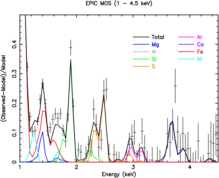
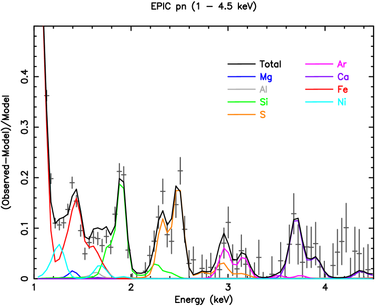
We show the effect in Fig. 3 using the spectrum of Sérsic 159-03. The plot shows the line contributions of the elements that contribute the most to the 1.0–4.5 keV band. Between roughly 1 and 2.5 keV, the lines in pn appear to contain less flux than their equivalents in MOS, which is in line with the differences we found between the two instruments. The effect is most notable at 1.4 keV, where the magnesium abundance is used by the fit to make up for the difference in flux. Because the flux of the iron feature at that energy is firmly coupled to the iron-K line complex, the magnesium line flux is the only one that can fill the gap in flux. The silicon line, however, is quite clean. But there is still a difference in flux at the position of this line. At higher energies between 2.5 and 4.5 keV, there is no significant effect anymore, which suggests that the sulfur and argon abundances are clean. Above 5 keV, there is a small difference in the slope that can influence the temperature and subsequently the calcium, iron, and nickel line fluxes.

Because abundances are directly derived from these line fluxes, we should be able to see the differences in the measured abundances. In Fig. 4, we show the abundance ratios for MOS and pn separately. We use the data of Sérsic 159-03 as an example, because it is representative for the whole sample. The values for the sulfur, argon, and calcium abundances appear to be consistent within errors in the two instruments. However, the silicon and magnesium abundances are clearly not. From spectral fits to the pn spectra we obtain systematically lower abundances for silicon and magnesium relative to MOS.

In order to check whether the systematic differences in the abundances are largely due to effective area effects, we fit the Sérsic 159-03 spectra again with corrected effective areas. We correct the MOS effective area with a simple broad-band spline model such that it nearly matches the pn effective area over the whole band. We do the same for pn. The filled symbols in Fig. 4 show the corrected abundances. The corrected MOS abundance is consistent with the original pn abundance and vice versa. Therefore, we can conclude that the effective area is the main contributor to the systematic differences between abundances determined with MOS and pn.

We choose to use a conservative approach and estimate the systematic error from Fig. 4. There are three elements that suffer from systematic effects: magnesium, silicon, and nickel. The systematic error in magnesium has such a large magnitude that we can not obtain a significant value for it. For silicon and nickel we calculate the weighted average and add the systematic error linearly to the statistical error. The error should be large enough to cover both the MOS and pn results. Using this method, we derive the following systematic errors (relative error with respect to the average abundance value): Si ($\pm$11%) and Ni ($\pm$19%).

Figure 4: Comparison between the abundances measured with the MOS and the pn instruments in the cluster Sérsic 159-03. We plot the abundance ratios with respect to iron. The open symbols correspond to the original data. The filled symbols show the results when the effective area is corrected to match the effective area of the other instrument.

3.2.3 Intrinsic scatter

In Fig. 5 we show the abundance ratios of S/Fe and Ca/Fe for the individual clusters. At first sight, the abundance ratios appear to be consistent with being flat, but they have a small scatter. In principle we expect to find a scatter, because the clusters in our sample are morphologically different and may have had different chemical evolution history. The intrinsic differences between the clusters need to be taken into account if we can detect the scatter with high significance.

In order to quantify this intrinsic scatter in the abundances, we calculate the error-weighted average of the abundances (see Table 4) with an error as described in Eq. 1:

$$\sigma_{\mathrm{tot}}^{2}=\sigma_{\mathrm{m}}^{2}+\sigma_{\mathrm{int}}^{2}$$ (1)

The value for the measured uncertainty ($\sigma_{\mathrm{m}}$) is known from the spectral fits, but the combined uncertainty ($\sigma_{\mathrm{tot}}$) and the intrinsic scatter in the population of clusters ($\sigma_{\mathrm{int}}$) are yet to be determined. We do this by varying $\sigma_{\mathrm{int}}$ until the $\chi_{\mathrm{red}}^{2}$ of the weighted average is equal to 1. The variance in the $\chi^{2}$ distribution for $n$ free parameters is $2n$ by definition. We use this variance to find the 1$\sigma$ limits on our estimate for $\sigma_{\mathrm{int}}$. The values we derive for $\sigma_{\mathrm{int}}$ are listed in Table 4.

We find that the intrinsic scatter ($\sigma_{\mathrm{int}}$) in the silicon and sulfur abundance ratios differs significantly from zero. This intrinsic scatter in the data needs to be included in the error of the weighted mean. Therefore, we use a new weighted mean for silicon and sulfur with $\frac{1}{\sigma_{\mathrm{tot}}^{2}}$ as weighing factor (see Table 4). Presumably due to lower statistics the $\sigma_{\mathrm{int}}$ of argon, calcium, and nickel does not show a significant deviation ($>3\sigma$) from zero, hence we may employ the original weighted means.

Figure 5: Plot of the S-Fe ratio (left) and the Ca-Fe ratio (right). In the Ca/Fe plot we do not plot clusters with 2$\sigma$ upper limits larger than 2.0 for plotting purposes (A1689, A3530, A3560, A3827 and A3888).

Table 4: Weighted averages of the abundance ratios with respect to solar (Lodders 2003) in our sample. Systematic uncertainties due to the effective-area calibration and uncertainties due to intrinsic scatter are included in the errors. The $\sigma_{\mathrm{int}}$ that we list here is the intrinsic scatter per data point.

X/Fe	Weighted mean	$\sigma_{\mathrm{int}}$
	(incl. $\sigma_{\mathrm{int}}$)
Si/Fe	0.66$\pm$0.13	0.17$\pm$0.05 †
S/Fe	0.60$\pm$0.06	0.18$\pm$0.06
Ar/Fe	0.40$\pm$0.03	0.11$\pm$0.05
Ca/Fe	1.03$\pm$0.04	0.12$\pm$0.08
Ni/Fe	1.41$\pm$0.31	0.2$\pm$0.2 †

†$\sigma_{\mathrm{int}}$ taken from PN data only.

3.2.4 Final abundance ratios

Now, we have derived values for the most relevant systematic uncertainties that affect our abundances. Using the total statistical uncertainty ($\sigma_{\mathrm{tot}}$) and the uncertainty in the effective area, we calculate the final abundance values with their errors. This final set of abundance ratios is shown in Table 4. Silicon and nickel are both dominated by the systematic uncertainty in the effective area. The sulfur abundance is dominated by the intrinsic scatter.

4 Discussion

We determined the elemental abundances in the core of 22 clusters of galaxies with XMM-Newton. Most of the abundances are not consistent with proto-solar abundances (Lodders 2003). The intrinsic scatter in the cluster abundance ratios is between 0–30%, which is quite small. Our sample consists of both relaxed and non-relaxed clusters as well as cooling and non-cooling core clusters. The small intrinsic scatter shows that the effects of merging, cooling and temperature structure on the abundance ratios is limited to 30% in cluster cores. We do not resolve a clear trend of abundances with the presence of a cooling-core.

It is a well established idea that most of the metals from oxygen up to the iron group are generated by supernovae. We construct a few models using elemental yields of supernova type Ia (SNIa) and core-collapse supernova (SNcc). This analysis is similar to the one described in Werner et al. (2006) and de Plaa et al. (2006).

We try several SNIa yields which we obtain from two physically different sets of supernova models (Iwamoto et al. 1999), namely slow deflagration and delayed detonation models. The W7 an W70 models describe a slow deflagration of the stellar core, while the other models are calculated using a delayed-detonation (DD) scenario. WDD2 is the currently favoured SNIa explosion scenario.

For the core-collapse supernovae we use the yields from a recent model by Nomoto et al. (2006). Note that with SNcc we mean all types of core-collapse supernovae including types II, Ib, and Ic. We integrate the yields from the model over the stellar population using an Initial-Mass Function (IMF). We perform the calculation following Tsujimoto et al. (1995):

$$M_{i}=\frac{\int_{10\leavevmode\nobreak\ \mathrm{M}_{\sun}}^{50\leavevmode\nobreak\ \mathrm{M}_{\sun}}\leavevmode\nobreak\ M_{i}(m)\leavevmode\nobreak\ m^{-(1+x)}\leavevmode\nobreak\ \mathrm{d}m}{\int_{10\leavevmode\nobreak\ \mathrm{M}_{\sun}}^{50\leavevmode\nobreak\ \mathrm{M}_{\sun}}\leavevmode\nobreak\ m^{-(1+x)}\leavevmode\nobreak\ \mathrm{d}m},$$ (2)

where $M_{i}(m)$ is the $i$th element mass produced in a star of main-sequence mass $m$. We use a standard model with Salpeter IMF ($x$=1.35) and solar-metallicity (Z=0.02).

For every element $i$ the total number of atoms $N_{i}$ is a linear combination of the number of atoms produced by a single supernova type Ia (Y_i,Ia) and type cc (Y_i,cc).

$$N_{i}=a\mathrm{Y}_{i,\mathrm{Ia}}+b\mathrm{Y}_{i,\mathrm{cc}},$$ (3)

where $a$ and $b$ are multiplicative factors of type SNIa and core-collapse supernovae respectively. The total number of particles for an element can be easily converted into a number abundance. This reduces to a system of two variables ($a$ and $b$) and six data points (Si, S, Ar, Ca, Fe and Ni). The fits are independent of the values for the solar abundances, because they are divided out in the procedure. In essence, we fit the absolute abundances in the cluster. In the following sections, we present the ratio of the relative numbers of SNIa with respect to the total number of supernovae (SNIa + SNcc) that have enriched the ICM.

The supernova number ratios that we present, reflect the supernova ratio that is fitted to the abundances that we measure in the ICM. This does not necessarily correspond to the true ratio of supernova explosions in the entire cluster over its lifetime (Matteucci & Chiappini 2005). Because SNIa explode some time after the initial star burst, there may be a difference between the fractions of type Ia and core-collapse products locked up into stars. However, this delay time ($\lesssim$3 Gyr, Maoz & Gal-Yam 2004) is probably short with respect to the formation time scale of the cluster. Therefore, it is likely that the bulk of the metals formed before 0.1$t_{\mathrm{Hubble}}$. Because this enrichment timescale is an order of magnitude smaller than the Hubble time, the instantaneous recycling approximation (Tinsley 1980) is presumably a reasonable approximation in the case of clusters. Using this approximation implies that we ignore the stellar lifetimes and thus the delay with which some chemical elements are released from stars into the ICM (Matteucci & Chiappini 2005).

We can make a very rough estimate of the systematic uncertainty that we introduce in our supernova ratio when we adopt the instanteneous recycling approximation. Galactic evolution models provide an indication about how the O/Fe ratio behaves in and around galaxies (for example, Calura & Matteucci 2006). However, galactic models are based on specific assumptions and approximations. Therefore, they also contain systematic uncertainties that are not well known. The plots in Calura & Matteucci (2006), for example, suggest that the fraction of oxygen that is locked up in stars is about a factor of two higher then for iron. If this model is a reasonable representation of galactic evolution in clusters of galaxies, then we overestimate our SNIa/(SNIa+SNcc) ratio in clusters with respect to the true supernova ratio with about 40% at maximum.

4.1 Solar abundances

The abundance ratios of silicon, sulfur, and argon that we derive from the sample are lower then proto-solar abundance ratios determined by (Lodders 2003). If we fit a constant to the cluster abundance ratios, we obtain a $\chi^{2}$ of 418 for 5 degrees of freedom. This means that the chemical enrichment in cluster cores differs significantly from that in the solar neighbourhood.

In order to compare the supernova ratios in clusters with the solar ratio, we fit the supernova models to a constructed dataset with solar abundance ratios that have a nominal error of 5% on every data point. From this fit (with a $\chi^{2}$/dof of 64/4), we find a supernova type Ia (WDD2) contribution in the solar abundance of 0.15 ($\pm$ 0.08), which is actually similar to the value for our galaxy found by Tsujimoto et al. (1995). This suggests that the abundances in the Sun are probably dominated by core-collapse supernovae that usually produce nearly flat abundance ratios. However, by adopting the instantaneous recycling approximation we might underestimate the type Ia fraction for the solar neighbourhood with the same factor that we derived from the galactic evolution models by Calura & Matteucci (2006).

4.2 Supernova type Ia models by Iwamoto et al.

Table 5: Number ratios of supernovae type Ia over the total number of supernovae derived using SN Ia models by Iwamoto et al. (1999) and by (Badenes et al. 2006). The results are from a fit which contained the elements from silicon to nickel. We also list the results of the comparison to solar abundances.

Model	SNIa/SNIa+SNcc	$\chi^{2}$/dof
Constant		418/5
Solar	0.15 $\pm$ 0.08	64/4
W7	0.22 $\pm$ 0.06	152/4
W70	0.26 $\pm$ 0.07	104/4
WDD2	0.37 $\pm$ 0.09	84/4
WDD3	0.22 $\pm$ 0.06	105/4
CDD2	0.32 $\pm$ 0.08	86/4
Tycho	0.72 $\pm$ 0.17	26/4

Figure 6: Abundance ratios versus atomic numbers for the sample. We fit the supernova yield models for SN Ia (WDD2) and SNcc ($Z$=0.02 and Salpeter IMF). The black line shows the total fit, while the dotted and dashed lines represent the SN Ia and SNcc models respectively.

We now try to fit the current supernova models to the data of the sample. In Table 5 we show the fit results using the supernova type Ia models W7, W70, WDD2, WDD3, and CDD2. None of the models provides an acceptable fit. The model with the lowest $\chi^{2}$ is the delayed-detonation model WDD2 ($\chi^{2}$/dof = 84/4).

The reason why the models fail can be found in Fig. 6. The calcium abundance is highly underestimated by the models. Moreover, the high calcium abundance forces the fit to increase the SNcc contribution. The current models are clearly not able to produce the observed Ar/Ca and Ca/Fe abundances. This result re-affirms the earlier measurements in 2A 0335+096 (Werner et al. 2006) and Sérsic 159-03 (de Plaa et al. 2006).

4.3 Supernova type Ia models based on Tycho

Figure 7: Same as Fig 6, but now we fit the SNIa yields found in the Tycho supernova remnant by Badenes et al. (2006). The nickel yield of the Tycho SNIa model was kindly provided by Carles Badenes (priv. comm.).

Recently, Badenes et al. (2006) compared type Ia models by Chieffi & Straniero (1989) and Bravo et al. (1996) to XMM-Newton EPIC observations of the Tycho supernova remnant. The Tycho supernova is thought to have been a type Ia supernova. Badenes et al. (2006) empirically modified the parameters of their delayed-detonation model to fit the Tycho observations. The parameter that mainly determines the outcome of their model is the density where the subsonic wave, which runs through the white dwarf during the explosion, turns into a supersonic shock. This transition from deflagration to detonation is put in by hand in every DD model. By modifying this parameter and the ratio between the specific internal energies of ions and electrons ($\beta$), they found a best-fit delayed-detonation model that fitted the Tycho observations.

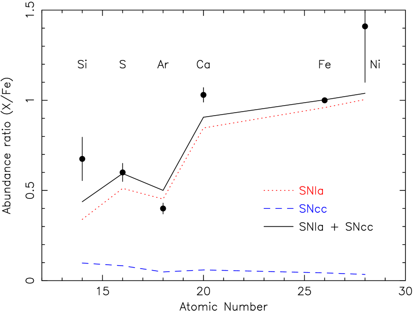
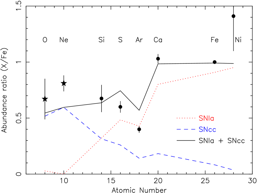
We take the yields from this best-fit model of Tycho and use them as a supernova type Ia model in our fit to the cluster abundances. Note that in Tycho not all the ejected material is visible in X-rays, because the reverse shock has not ionised all the material yet. Therefore, the Tycho results might not reflect the total SNIa yields yet. Despite this caveat, the Tycho model provides a major improvement in $\chi^{2}$ compared to the Iwamoto et al. (1999) models (see Table 5). In Fig. 7, we show that the Tycho model is more successful in fitting the calcium abundance in clusters. Moreover, the supernova ratios change dramatically, the SNIa/(SNIa+SNcc) ratio for this model is 0.72 $\pm$ 0.17.

This shows that the Ar/Ca and Ca/Fe abundance ratios mainly determine how well type Ia models fit. By varying the parameters of the delayed-detonation models, it is in principle possible to obtain a calcium abundance that fits the observations, which apparently very effectively constrain type Ia models.

4.4 Core-collapse models

In order to test whether our models are also reproducing the core-collapse contribution adequately, we need abundances of some typical core-collapse products. Therefore, we estimate the oxygen and neon abundance of the sample using the Reflection Grating Spectrometer (RGS) aboard XMM-Newton. For oxygen, we take the average of the clusters Sérsic 159-03 and 2A 0335+096, because these clusters have the highest exposure in our sample and very good RGS data (de Plaa et al. 2006; Werner et al. 2006). The O/Fe measurements of the two clusters are not statistically consistent possibly due to systematic differences in the line widths (see de Plaa et al. 2006, for an explanation of this effect). Therefore, we take the average value and assign an error which covers both results within 1$\sigma$. The neon abundance is consistent in both Sérsic 159-03 and 2A 0335+096, hence we take the weighted average of the two neon abundances and use them in the rest of the fits.

Figure 8: Fit using the SNIa yields by Badenes et al. (2006), but now with additional oxygen and neon data points (stars) obtained from the RGS spectra of Sérsic 159-03 and 2A 0335+096. Here, the core-collapse model with $Z$=0.02 and Salpeter IMF is used.

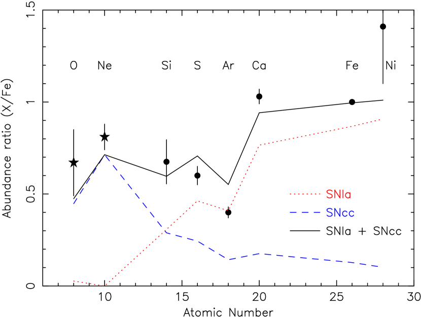
The fit including O/Fe and Ne/Fe from RGS is shown in Fig. 8. We use here a standard core-collapse model ($Z$=0.02 and Salpeter IMF) and the type Ia model based on Tycho. The trend in O/Ne that is predicted by the core-collapse model, is consistent with the O/Ne ratio that we observe. However, the core-collapse contribution needs to increase with respect to the model used in Fig. 7 to explain the absolute values for O/Fe and Ne/Fe (see Table 6). The typical values that we derive are of the order of 45–60%. Considering the uncertainties, this number is compatible with the current supernova type Ia ratio within $z$=0.03 ($\sim$42%) determined by the Lick Observatory Supernova Search (LOSS) (van den Bergh et al. 2005).

In principle, the increase of the core-collapse contribution with respect to the results before we included oxygen an neon results in a smaller predicted Ar/Ca ratio. However, the data suggest that the Ar/Ca ratio is larger. The plot shows that this particular core-collapse model still allows a relatively high Ar/Ca ratio, because the absolute contributions of silicon, sulfur, argon, and calcium are relatively small in this model.

4.4.1 Effect of progenitor metallicity on core-collapse yields

Figure 9: Fit using the SNIa yields by Badenes et al. (2006) and SNcc yields for Z=0.001 metallicity progenitors (Nomoto et al. 2006).

Table 6: Results for a supernova fit to the abundance ratios using SNcc models by Nomoto et al. (2006) that are integrated over a Salpeter ($x$=1.35) or “top-heavy” IMF ($x$=0). $Z$=0.02 is the solar abundance. For the type Ia model we used Badenes et al. (2006).

$Z$	Salpeter IMF		“Top-heavy” IMF
	$\frac{SNIa}{SNIa+SNcc}$	$\chi^{2}$/dof	$\frac{SNIa}{SNIa+SNcc}$	$\chi^{2}$/dof
0	0.55$\pm$0.05	79/6	0.68$\pm$0.04	102/6
0.001	0.51$\pm$0.05	54/6	0.62$\pm$0.04	69/6
0.004	0.49$\pm$0.05	55/6	0.62$\pm$0.04	58/6
0.02	0.44$\pm$0.05	40/6	0.57$\pm$0.04	34/6

Up to now, we have used a core-collapse supernova model that assumes that the progenitor had a solar metallicity. Nomoto et al. (2006) also provide models where the metallicity ($Z$) of the supernova progenitor is 0, 0.001, and 0.004. In Table 6 we show the results for the fits using progenitor metallicities ranging from 0 to 0.02 (solar). The Z=0.001, Z=0.004, and Z=0.02 models do show a relatively small variation in $\chi^{2}$. The data are still compatible with a wide range of metallicities (0.001-0.02).

In Fig. 9 we show the fit result for the Z=0.001 model. The main difference between this $Z$=0.001 model and the $Z$=0.02 model is the amount of oxygen and neon produced. The neon peak is clearly less pronounced compared to the model in Fig. 8, while the plateau from silicon to nickel in the core-collapse contribution is nearly unaffected. That also confirms that the influence of metallicity differences in SNcc models on the Ar/Ca ratio is limited.

4.4.2 Effect of IMF on core-collapse yields

Figure 10: Fit using the SNIa yields by Badenes et al. (2006) and SNcc yields for Z=0.001 metallicity progenitors (Nomoto et al. 2006) that are integrated over a “top-heavy” IMF.

We also fit the data for core-collapse models integrated over a “top-heavy” IMF ($x$=0), because presumably more high-mass stars form in low-metallicity environments. Table 6 shows that the fits are similar to the fits using Salpeter IMF. In Fig. 10, we show the fit for this metallicity. The main differences with Salpeter IMF models are in the O/Ne ratio. The abundance peak in the model is shifted from neon to oxygen with respect to the Salpeter models, which is less consistent with the neon abundance from RGS. Again, the plateau from silicon to nickel in the core-collapse model is barely affected.

4.5 The fraction of low mass stars that become Type Ia SNe

This study indicates a much higher lifetime averaged ratio of type Ia to core-collapse supernovae than in the Galaxy. The reason for this large contribution of SNIa is likely that in late type galaxies, like our own galaxy, ongoing star formation ensures an ongoing core collapse contribution. For clusters of galaxies, the star formation continued at a very reduced level shortly after the formation of the cluster. This has some interesting consequences. SNIa are likely the result of a thermonuclear runaway explosion of a C-O white dwarf in binary systems, caused by accretion from the secondary star. Since this involves the formation of a white dwarf from a star with mass $M\lesssim 10\leavevmode\nobreak\ \mathrm{M}_{\sun}$, there is a considerable delay between the period of star formation and the resulting SNIa explosion. In late type galaxies the subsequent waves of star formation make it difficult to disentangle the SNIa contribution from recent and old star formation periods. However, cluster of galaxies are an interesting laboratory to study the fraction of all stars that will eventually become type Ia supernovae, since the star formation has shut down, and for the last few Gyr since formation, the buffer of potential type Ia progenitors has nearly emptied.

As a result, the fraction of SNIa in clusters must be a good approximation to the fraction of low mass stars that can become type Ia explosions. For a power law initial mass function we can write (Yoshii et al. 1996):

$$\frac{SNIa}{SNIa+SN_{cc}}=\frac{f_{SNIa}\int_{M_{low}}^{M_{cc}}m^{-(1+x)}dm}{f_{SNIa}\int_{M_{low}}^{M_{cc}}m^{-(1+x)}dm+\int_{M_{cc}}^{M_{up}}m^{-(1+x)}dm},$$ (4)

with $M_{low}$ the lower limit to the mass of stars that can have contributed to the type Ia production, and $M_{up}$ the mass of the most massive stars. The parameter of interest here is $f_{SNIa}$, which is defined as the fraction of stars with $M_{low}<M<M_{cc}$ that will eventually explode as SNIa.

Table 7: The fraction, $f_{SNIa}$, of low mass stars in the range $M_{low}$ to $M_{cc}$ that will eventually result in SNIa. It is based on our observed SNIa fraction of $\frac{SNIa}{SNIa+SNcc}=0.44\pm 0.10$.

	$M_{low}=0.9\leavevmode\nobreak\ \mathrm{M}_{\sun}$	$M_{low}=1.5\leavevmode\nobreak\ \mathrm{M}_{\sun}$
Salpeter IMF ($x=1.35$)
$M_{cc}=8\leavevmode\nobreak\ \mathrm{M}_{\sun}$	$4.1\pm 1.7$%	$9\pm 4$%
$M_{cc}=10\leavevmode\nobreak\ \mathrm{M}_{\sun}$	$2.9\pm 0.1$%	$6\pm 3$%
Kroupa (2002)
$M_{cc}=8\leavevmode\nobreak\ \mathrm{M}_{\sun}$	$2.0\pm 0.8$%	$4.0\pm 1.7$%
$M_{cc}=10\leavevmode\nobreak\ \mathrm{M}_{\sun}$	$1.3\pm 0.6$%	$2.7\pm 1.1$%

It is clear that the absolute lower limit to $M_{low}$ is the mass of stars that can evolve to a C-O white dwarf within a Hubble time, about 0.9 $\mathrm{M}_{\sun}$. However, in order to have sufficient mass available in the binary to push the white dwarf over the Chandrasekhar limit, it is usually assumed that the total mass of a binary producing a SNIa explosion should exceed $\sim$ 3 $\mathrm{M}_{\sun}$ (Matteucci & Recchi 2001). This implies that the initial mass of the primary star $\gtrsim$ 1.5 $\mathrm{M}_{\sun}$.

The time scale for producing a Type Ia supernova is most likely determined by the evolution of the secondary, i.e. roughly by the duration of the main sequence. If the secondary is 0.9 $\mathrm{M}_{\sun}$, this corresponds roughly to a Hubble time, but there is considerable evidence that the mean delay time between star formation and type Ia explosion is shorter, namely of the order of 1 Gyr. Strolger et al. (2004) find a value of 2-4 Gyr. However, based on a lack of observed SNIa in clusters of galaxies, Maoz & Gal-Yam (2004) find a 2$\sigma$ upper-limit of about 3 Gyr for the delay time. Very recently Mannucci et al. (2006) argued for two channels for SNIa explosions, one with a very short delay time of $10^{8}$ yr, and the other with 2-4 Gyr. In other words, the majority of the type Ia explosions must occur in binaries where the secondary star has a lifetime shorter than 2-4 Gyr. The mass of the secondary star that corresponds to such lifetimes is about 1.25–1.5 $\mathrm{M}_{\sun}$ (Greggio & Renzini 1983). In the extreme case, where the delay time is $\lesssim$ 2 Gyr, $M_{low}$ would be about 1.5 $\mathrm{M}_{\sun}$.

Table 7 shows the values for $f_{SNIa}$ using different assumptions for $M_{low}$, $M_{cc}$ and the initial mass function. We use the best fit SNIa rate of $0.44\pm 0.10$ (Table 6), but with slightly larger errors in order to allow for systematic uncertainties. The values that we find for $M_{low}=1.5\mathrm{M}_{\sun}$ are high compared to previous results based on other observational data, which suggests $f_{SNIa}=1-5$% (Greggio & Renzini 1983; Yoshii et al. 1996; Matteucci & Recchi 2001). Note that these authors sometimes use slightly different definitions for $M_{low}$ and $M_{cc}$. Our lowest value is 1.3%, which assumes $M_{cc}=10\leavevmode\nobreak\ \mathrm{M}_{\sun}$ and $M_{low}=0.9\leavevmode\nobreak\ \mathrm{M}_{\sun}$ together with the broken power law IMF of Kroupa (2002). Notice also that $f_{SNIa}$ refers to all stars with masses between $M_{low}$ and $M_{cc}$. We can estimate the probability that a binary produces a type Ia supernova from the value of $f_{SNIa}$. We assume that roughly 50% of all stars are formed in binaries, which introduces a factor of two. In addition, we need another factor of two because we want to count binaries instead of stars. Together, the probability that a binary produces a SNIa supernova is thus about four times higher then $f_{SNIa}$.

Our derived supernova ratios therefore suggest that binary systems in the appropriate mass range are very efficient in eventually forming SNIa explosions ($\sim$ 5–16%, depending on the assumptions for the IMF and $M_{cc}$). We are aware that we ignore several complications in this simple calculation, such as an increased binarity fraction for massive stars that flattens the IMF for binary stars and binary mass ratios that may peak near 1. Also the instanteneous recycling approximation may introduce an additional uncertainty. However, a detailed calculation is beyond the scope of this paper.

5 Conclusions

We measure the abundances for silicon, sulfur, argon, calcium, iron, and nickel in a sample of clusters with XMM-Newton (EPIC), and we add a high-resolution oxygen and neon measurement from RGS (de Plaa et al. 2006; Werner et al. 2006). From these data we conclude that:

• The Ar/Ca ratio in clusters is a good touchstone for determining the quality of type Ia models. The core-collapse contribution, which is about 50% and not strongly dependent on the IMF or progenitor metallicity, does not have a significant impact on the Ar/Ca ratio.

• Current supernova type Ia models (Iwamoto et al. 1999) do not agree with our data, because they fail to produce the Ar/Ca and Ca/Fe abundance ratios.

• A major improvement of the supernova fits is obtained, when we use an empirically-modified supernova type Ia model, which is calibrated on the Tycho supernova remnant (Badenes et al. 2006). This model largely solves the problems with the Ar/Ca and Ca/Fe abundance ratios by varying the density where the sound wave in the supernova turns into a shock and varying the ratio of the specific internal energies of ions and electrons at the shock.

• The number ratio between supernova type Ia and core-collapse supernovae suggests that binary systems in the appropriate mass range are very efficient ($\sim$ 5–16%) in eventually forming supernova type Ia explosions.

• We find that the progenitors of the core-collapse supernovae which contributed to the ICM abundances have probably been enriched. Progenitor abundances range from $Z\sim$0.001 to $Z\sim$0.02.

• The intrinsic spread in abundance ratios between clusters is smaller than 30%. That means that the chemical histories of the clusters do not depend a lot on cluster temperature, temperature structure or merging activity.

Appendix A Abundance data

In Table 8 we list the abundances obtained from fits to the EPIC data. The MOS and pn spectra are fitted simultaneously. We included a systematic error in the uncertainties on the Si/Fe and Ni/Fe abundance ratios (see Sect. 3.2.2 for a discussion about systematic errors).

Table 8: Abundance ratios in the sample of clusters with respect to the solar abundances determined by Lodders (2003). The listed ratio is calculated using $\frac{X/X_{\sun}}{Fe/Fe_{\sun}}$. We included a systematic error in the data points of Si/Fe and Ni/Fe. See Sect. 3.2.2 for a discussion about systematic errors.

Cluster	Si/Fe	S/Fe	Ar/Fe	Ca/Fe	Ni/Fe	Fe
2A 0335	0.78 $\pm$ 0.09	0.636 $\pm$ 0.019	0.43 $\pm$ 0.04	0.95 $\pm$ 0.06	1.4 $\pm$ 0.4	0.741 $\pm$ 0.006
A 85	0.72 $\pm$ 0.18	0.61 $\pm$ 0.15	0.4 $\pm$ 0.4	1.4 $\pm$ 0.4	1.0 $\pm$ 0.7	0.574 $\pm$ 0.018
A 133	0.64 $\pm$ 0.14	0.40 $\pm$ 0.09	0.6 $\pm$ 0.2	1.3 $\pm$ 0.3	1.6 $\pm$ 0.6	0.81 $\pm$ 0.02
A 1651	0.0 $\pm$ 0.4	0.3 $\pm$ 0.4	0.0 $\pm$ 0.4	0.0 $\pm$ 0.6	1.4 $\pm$ 1.3	0.45 $\pm$ 0.03
A 1689	0.3 $\pm$ 0.4	1.1 $\pm$ 0.4	0.8 $\pm$ 1.0	0.6 $\pm$ 0.9	0.6 $\pm$ 1.0	0.40 $\pm$ 0.02
A 1775	0.57 $\pm$ 0.18	0.77 $\pm$ 0.14	0.5 $\pm$ 0.3	1.7 $\pm$ 0.4	1.6 $\pm$ 0.7	0.63 $\pm$ 0.02
A 1795	0.75 $\pm$ 0.14	0.34 $\pm$ 0.08	0.2 $\pm$ 0.2	1.1 $\pm$ 0.3	1.3 $\pm$ 0.5	0.517 $\pm$ 0.009
A 2029	0.4 $\pm$ 0.2	0.32 $\pm$ 0.17	0.00 $\pm$ 0.10	1.3 $\pm$ 0.5	1.6 $\pm$ 0.7	0.587 $\pm$ 0.017
A 2052	0.74 $\pm$ 0.12	0.76 $\pm$ 0.05	0.55 $\pm$ 0.11	1.35 $\pm$ 0.16	1.4 $\pm$ 0.4	0.682 $\pm$ 0.011
A 2199	0.73 $\pm$ 0.13	0.60 $\pm$ 0.07	0.60 $\pm$ 0.16	1.04 $\pm$ 0.19	1.5 $\pm$ 0.5	0.532 $\pm$ 0.008
A 2204	0.75 $\pm$ 0.18	1.32 $\pm$ 0.19	0.0 $\pm$ 0.2	1.6 $\pm$ 0.6	1.6 $\pm$ 0.7	0.59 $\pm$ 0.02
A 2589	0.55 $\pm$ 0.14	0.58 $\pm$ 0.10	0.4 $\pm$ 0.2	1.2 $\pm$ 0.3	1.8 $\pm$ 0.6	0.666 $\pm$ 0.019
A 3112	0.70 $\pm$ 0.14	0.67 $\pm$ 0.09	0.5 $\pm$ 0.2	1.3 $\pm$ 0.3	1.9 $\pm$ 0.6	0.695 $\pm$ 0.016
A 3530	1.1 $\pm$ 0.6	1.1 $\pm$ 0.6	0.3 $\pm$ 0.9	1.2 $\pm$ 1.5	0.0 $\pm$ 2.0	0.28 $\pm$ 0.04
A 3558	0.74 $\pm$ 0.16	0.41 $\pm$ 0.12	0.3 $\pm$ 0.3	1.6 $\pm$ 0.4	1.5 $\pm$ 0.6	0.478 $\pm$ 0.017
A 3560	0.9 $\pm$ 0.3	0.4 $\pm$ 0.3	0.2 $\pm$ 0.5	1.0 $\pm$ 1.0	1.1 $\pm$ 1.3	0.39 $\pm$ 0.03
A 3581	0.80 $\pm$ 0.10	0.75 $\pm$ 0.04	0.66 $\pm$ 0.09	1.32 $\pm$ 0.16	1.3 $\pm$ 0.4	0.654 $\pm$ 0.013
A 3827	0.2 $\pm$ 0.3	0.0 $\pm$ 0.4	0.0 $\pm$ 0.7	2.9 $\pm$ 1.2	1.1 $\pm$ 1.2	0.38 $\pm$ 0.03
A 3888	0.1 $\pm$ 0.5	1.8 $\pm$ 1.1	0.0 $\pm$ 1.3	1.0 $\pm$ 1.9	0.0 $\pm$ 1.8	0.30 $\pm$ 0.03
A 4059	0.59 $\pm$ 0.13	0.45 $\pm$ 0.07	0.16 $\pm$ 0.17	0.7 $\pm$ 0.2	1.0 $\pm$ 0.5	0.687 $\pm$ 0.014
MKW 3s	0.84 $\pm$ 0.13	0.63 $\pm$ 0.07	0.54 $\pm$ 0.18	1.2 $\pm$ 0.2	1.4 $\pm$ 0.5	0.551 $\pm$ 0.011
S 159-03	0.67 $\pm$ 0.10	0.55 $\pm$ 0.03	0.41 $\pm$ 0.07	0.87 $\pm$ 0.10	1.6 $\pm$ 0.4	0.533 $\pm$ 0.005