Galactic Basins of Helium and Iron around the Knee Energy

Antonio Codino¹, François Plouin²

¹⁾ INFN and Dipartimento di Fisica dell’Universita degli Studi di Perugia, Italy.
²⁾ former CNRS researcher, LLR, Ecole Polytechnique, F-91128 Palaiseau,France.

The differential energy spectrum of cosmic rays exhibits a change of slope, called $knee$ of the spectrum, around the nominal energy of $3\times 10^{15}$ $eV$, and individual $knees$ for single ions, at different energies. The present work reports a detailed account of the characteristics and the origin of the knees for Helium and Iron. Current observational data regarding the magnetic field, the insterstellar matter density, the size of the Galaxy and the galactic wind, are incorporated in appropriate algorithms which allow to simulate millions of cosmic-ion trajectories in the disk. Bundles of ion trajectories define galactic regions called basins utilized in the present analysis of the knees. The fundamental role of the nuclear cross sections in the origin of the helium and iron knees is demonstrated and highlighted.

The results of the calculation are compared with the experimental data in the energy interval $10^{12}$ $eV$ - $5\times 10^{17}$ $eV$. There is a fair agreement between the computed and measured energy spectra of Helium and Iron; rather surprisingly their relative intensities are also in accord with those computed here. The results suggest that acceleration mechanisms in the disk are extraneous to the origin of the $knees$.

PACS:11.30.Er; 13.20.Eb; 13.20Jf; 29.40.Gx; 29.40.Vj This text appeared as the LNF report INFN/TC-06/05. See the link: http://www.lnf.infn.it/sis/preprint/pdf/INFN-TC-06-5.pdf

1 Introduction

In a recent companion paper [1] the notion of galactic basin was adopted in order to investigate some properties of galactic cosmic rays. This concept, introduced in a previous work [2], is extensively utilized in this study. The concept of galactic basin is similar to that of a terrestrial basin, peculiar of a river, with all the $caveats$ inherent to any analogy. When the position of an instrument recording the passage of cosmic ions and the source distribution in the disk are assigned, the galactic basin is simply that particular region populated by the majority of the sources feeding the instrument. Changing the position of the instrument, the characteristics of the $basin$ (volume, extension, shape, contour, etc) are altered. In our opinion, the concept of galactic basin is simple and straightforward, and particularly useful when an efficient tool is required to compare, investigate or even discover some properties of cosmic ions.

The purpose of this study is to identify those physical phenomena at the origin of the $knee$ and to give a quantitative account of the major characteristics of the helium and iron $knees$. Their explanation is a part of a research effort to account for the knees and ankles of individual ions. The origin of the $knees$ presented here are conclusively corroborated in a forthcoming, collateral paper [3] demonstrating the interconnection between the $knees$ and $ankles$ of individual ions of the cosmic-ray spectrum.

The results and the prerequisites of this investigation are organized as follows. In the second Section the hypotheses and the parameters involved in the calculation are enumerated. Since they have been presented in previous studies [4,5,6], their description is concise. Only for two upgrades of the simulation code ($Corsa$), the description is ampler; these upgrades are introduced here for the first time. They regard the galactic wind and the propagation of the particles at energies greater than $5\times 10^{11}$ $eV/u$, the previous limit in the maximum energy of $Corsa$. In Section 3 the properties of galactic basins of Helium and Iron, in the interval $10^{12}$ and $5\times 10^{17}$ $eV/u$, are summarized and discussed. Through many examples, it is investigated how the shape of basins change with increasing energy. In Section 4 are clarified and consolidated some results given in Section 2. In Section 5 it is investigated in detail how nuclear cross sections affect the change of the spectral index of individual ions. The interaction cross sections of Helium and Iron with the insterstellar matter are set artificially constant. Then the differential energy spectrum of Helium and Iron is studied by counting the number of cosmic rays intercepting the local galactic zone. In Section 6 the influence of the magnetic field and the galactic wind on the results previously obtained is calculated and discussed. In Section 7 a comparison of the predicted and measured energy spectra of Helium and Iron is presented. Unfortunately, even a concise comparison (to preserve a tolerable length of the paper) with the experimental data necessitates logical and theoretical prerequisites, partially presented in Section 7, partially described elsewhere [7,8].

Protons are not included in this analysis, in spite of their importance, because, at very high energy, computational procedures become quite complex and very time consuming. Primary protons interacting with the interstellar hydrogen yield many secondaries, indistinguishable from primaries, which make the analysis of the results quite involved as reported in a previous study limited to the energy of $10^{11}$ $eV$ [4]. The present calculation deals only with Helium and Iron because the behavior of all other ions lighter than Iron, except protons, fall between these two nuclei, as previously demonstrated [1]. The energy interval considered extends from $10^{12}$ to $5\times 10^{17}$ $eV/u$, which is adequate for the $knee$ problem.

2 Observational data incorporated in the simulation algorithms

In the following the set of parameters utilized in the calculation are concisely presented. The form and dimensions of the Galaxy are displayed in fig. 1.

Figure 1: Lateral and top view of the galactic disk indicating the local zone and the Bulge.

A cylindrical frame of reference is used with coordinates $r$, $z$ and $\phi$. The Bulge is an ellipsoid with a major axis of $8$ $kpc$, lying onto the galactic midplane, and a transverse minor axis of 6 $kpc$. The disk has a radius of $15$ $kpc$ and a half thickness of $250$ $pc$. The interstellar matter consists of pure hydrogen with constant density of 1 atom $per$ $cm^{3}$ [9] enhanced to 1.24 to take into account heavier nuclei. The galactic magnetic field is a superposition of regular and chaotic fields. In fig. 3 are shown the line pattern of the spiral field and the principal field line (thick line) which intercepts the Earth at coordinates $r$=8.5 $kpc$, $z$=$0$ $kpc$ and $\phi$=$90$ $degrees$. The field strength of the regular component is shown in fig. 2. The coherence length of the regular field is $125$ $pc$ [12].

Figure 2: Pattern of field lines of the spiral magnetic field projected onto the galactic midplane. The spiral field line (thick line) departing from the bulge, intercepting the local galactic zone and terminating on the disk frontier ($r$ = 15 $kpc$) is called the principal field line.

Figure 3: Magnetic field strength in the disk. Note that the axis of the disk height has a different scale from that representing the disk radius.

The chaotic field is materialized by magnetic cloudlets [ see, for example, references 10,11] of spherical form with a mean radius of 2.5 $kpc$ fluctuated by a uniform distribution with a width of $0.5$ $pc$. The ion propagation normal to the regular spiral field is generated by the chaotic field leading to a transverse-to-longitudinal displacement ratio of 0.031, in a range compatible with the quasi-linear theory of ion propagation in an astrophysical environment [13].

The source distribution, $Q(r,z,\phi)$, regarded as uniform, is the following :

$$Q(r,z,\phi)=C\theta(r-R)N(\sigma,z)\quad\quad\quad(1)$$

where $C$ is a normalization constant, $\theta$ is the radial distribution with a disk radius $R$ = $15$ $kpc$ and N($\sigma$,$z$) is the vertical distribution with a gaussian shape with standard deviation $\sigma$ = $80$ $pc$. The function N($\sigma$,$z$) makes smooth the source distribution along $z$ with respect to a steep, unphysical, $z$-rectangular distribution. The function $Q(r,z,\phi)$ is not dissimilar to the positions of the galactic sources distributed as supernovae remnants [14,15] with the advantage of avoiding a specific, constraining hypothesis on source positions. Replacing N($\sigma$,$z$) by $\theta(z-z_{0})$ in equation (1), a strictly uniform distribution is obtained where $z_{0}$ is the disk half thickness. The mean distance of the source positions from the local zone is denoted by $D_{si}$.

The flattening of the electron spectrum in external galaxies, detected by radiotelescopes at frequencies about 1 GHz, is commonly regarded as observational evidence for the existence of the galactic winds [16]. This evidence is less convincing in the Milky Way because, the synchrotron radiation detection and analysis of the results are quite complex, being the Earth embedded in the Galaxy. A three dimensional formula, based on observational data, for the galactic wind in the disk and halo volume, is not known. Usually, a one dimensional wind along $z$ with a linear velocity is considered in many investigastions of cosmic rays, though a radial wind component is not excluded [17]. From these inputs it seems appropriate for this calculation a linear formula of the type:

$$v(z)=az\quad\quad\quad\quad\quad\quad(2)$$

where $a$ is a suitable constant constrained by the maximum wind velocity, $v_{max}$, at the disk boundaries. Simulation algorithms shift along $z$ the trajectory segments by the amount $\delta_{z}$ according to the equation (2), namely, $\delta_{z}$ = $v$($z$)$\tau$ where $\tau$ is the time interval taken by the cosmic ion to travel the length $l_{z}$ of the trajectory segment along $z$. The maximum wind velocities adopted in a variety of cosmic-ray investigations in the disk, span the range 5 to 40 $km$/$s$. The account of the Boron-to-Carbon flux ratio at very low energy [18] probably represents an incisive example of the role of the galactic wind on cosmic rays. Instead of adopting a particular value of $v_{max}$, which is unnecessary in this work as it will be clear in Sections 6 and 7, the parameter $a$ and the related maximum wind velocity, is left as a free parameter.

New algorithms have been added for the propagation of cosmic rays around the knee energy. The maximum energy of the previous version of $Corsa$ was at $5\times 10^{11}$ $eV/u$.

Figure 4: Qualitative illustration of the sizes of three helices in the galactic magnetic field. The field is aligned along the straight line $AB$ and it can be a chaotic or a regular field segment. A particle of low energy, initially at the point $A$ with velocity $\alpha$, will closely follow the magnetic field, with a small helix radius, reaching the point $B$ with a velocity $\beta$. In this case the velocity vectors $\alpha$ and $\beta$ are randomly oriented (fully uncorrelated). A particle of sufficient high energy at $A$ with velocity $\alpha$, describing the ample helix from $A$ to $C$, leaves the point $C$ with the velocity vector $\gamma$. In this case, unlike the previous one, the vectors $\gamma$ and $\alpha$ are fully correlated. The vast majority of cosmic rays, having very low energy compared to the $knee$ energy, simply follows the regular field lines with a small tranverse displacement and their helix radii are so small to be indistinguishable from the segment $AB$ ( thick line ).

Fig. 4 reports, as an example, three helical trajectories winding round the magnetic field, whose direction coincides with the segment $AB$, $150$ $pc$ long. The radii of the three helices are 0.01, 4 and 50 $pc$ in a uniform field with $3$ $\mu$$G$ strength. The smallest helix is indistinguishable with the line segment $AB$, indicative of the fundamental, standard condition of cosmic ions in the Galaxy at energies below $10^{14}$ $eV/u$; while travelling in the Galaxy they are mainly bound to the lines of the regular field. Details of the propagation procedure at very high energy are given in the Appendix $B$.

Particles which enter the Halo are regarded as lost, since the albedo is less than 2 per cent at the energy of $10^{11}$ $eV$[1] and decreases with the energy. Either a circular or a spiral field can be used in the Halo with appropriate strength (see equation (3) of ref.[1]). Matter density in the Halo is a factor $10^{2}$-$10^{3}$ less than that in the disk. In the present investigation, however, the influence of the Halo and its size, is quite marginal.

3 Galactic basins around the knee energies

In this Section the major characteristics of the galactic basins are summarized. Note that the total length of the principal magnetic field line from the Bulge ($r$ = 4 $kpc$ ) to the disk radius ($r$ = 15 $kpc$) is 43.5 $kpc$.

In fig. 5 are shown the positions of the Helium sources having trajectories intercepting the local galactic zone at sixteen different energies (from $10^{12}$ to $4\times 10^{17}$ $eV/u$). The source positions are projected onto the galactic midplane. The sequence of the plots highlights the changes of the source distributions with increasing energy.

Figure 5: Different forms of the galactic basins projected onto the galactic midplane illustrating how they modify as the energy increases from $10^{12}$ to $4\times 10^{17}$ $eV$/$u$. Each figure derives from an initial sample of $2\times 10^{5}$ ions. The frame of reference and the position of the local zone are those shown in figure 2.

The corresponding spatial distributions of the iron sources (not shown) have similar structure, though the values of the parameters characterizing the basins are, of course, different. Source positions populate a narrow strip, along the principal magnetic field line, except at the maximum energy of $4\times 10^{17}$ $eV/u$ where the basin form is radically different from the previous ones. This fundamental feature was identified at low energy below $10^{11}$ $eV/u$, long time ago by ourselves, for proton and beryllium ions, and recently for all other ions from Helium to Iron [1]. These characteristics of the ion basins derive, ultimately, from observational data of the Milky Way, and particularly, from the spiral shape of the magnetic field shown in fig. 2. As a general rule, spiral galaxies possess a regular magnetic field with a spiral shape, Andromeda being a notable exception with an annular field. This feature, together with the small ratio of transverse-to-longitudinal ion propagation, yields long and narrow basins.

Fig. 6 displays a tridimensional view onto the galactic midplane of the positions of helium and iron sources emanating trajectories which intercept the local galactic zone in a reference frame where the horizontal axis is the principal field line.

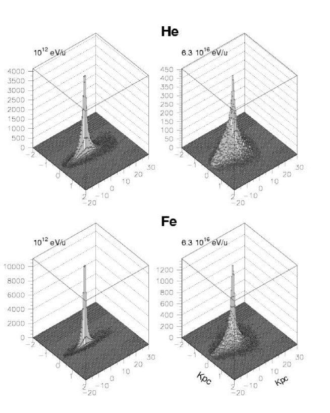
Figure 6: Spatial distribution of helium and iron sources in the Disk at the energies of $10^{12}$ and $6.3\times 10^{16}$ $eV/u$. The results are obtained with an initial sample of $200$ $000$ trajectories for both ions. The source arrays of the highest energy are typical of the $knee$ energy region.

This coordinate system and its advantages are described in Appendix A. Each plot contains samples of $2\times 10^{5}$ ion trajectories. To illustrate the basin profiles two arbitrary energies of $10^{12}$ and $6.3\times 10^{16}$ $eV/u$ are chosen. At the energy of $10^{12}$ $eV/u$ both basins are well contained in the Disk, the iron basin being more concentrated around the local zone because its trajectory lengths are shorter than those of Helium. At the energy of $10^{16}$ $eV/u$ both basins increasingly populate a zone toward the bulge frontier. Note that in fig. 6 the bulge lies at coordinate $-16.7$ $kpc$ along the principal field line, (i.e. the axis of the figure) while the disk edge at $24.1$ $kpc$.

The spatial distribution of the sources in fig. 6 can be visualized by contour plots containing $90\%$ of the sources. The arbitrary value of this percentage was previously adopted (see figure 5 of reference [1] ). Fig. 7 shows the contours of two Iron basins at the energies of $10^{12}$ and $6.3\times 10^{16}$ $eV/u$.

Figure 7: Contour plots containing $90\%$ of iron sources at the energy of $10^{12}$ and $6.3\times 10^{16}$ $eV$. The contours refer to same iron samples shown in fig. 6. The energy of the lower contour lies in the $knee$ energy region.

The lower and upper solid lines in fig. 7 delimit, respectively, the Bulge and the disk internal frontiers. In order to better emphasize the transversal structure of the basin, the horizontal axis in fig. 7 is magnified by a factor 50.

It is evident that the basin shape changes from an ovoidal form, typical at low energy, to a ram head, typical at high energy. These alterations of the basin shape suggest that cosmic-ray populations suffer difforming filtering and processing as the energy varies. It is apparent, for example, the basin enlargement with increasing energy. The supposed continuity between the two contour plots in fig. 7, passing from a narrow, ovoidal shape to a large ram-head shape, manifests the transverse enlargement with the increasing energy. Note also that the basin at $10^{12}$ $eV/u$ is well contained in the Disk, with longitudinal ends approximately equidistant from the bulge and disk frontiers. On the contrary, at the energy of $6.3\times 10^{16}$ $eV/u$ the longitudinal ends of the basin are not equidistant from the bulge and disk frontiers. The relative high clustering of cosmic-ion sources closer to the Bulge frontier ($r$ = 4 $kpc$) is due to the magnetic field strength, quite large in this zone ($4-6\mu$$G$) compared to the strength ($0.5-1\mu$$G$) around the disk edge ($r$ = 15 $kpc$) as indicates fig. 3.

The basin extension is characterized by the length $L_{B}$, along the principal field line, and the transverse width $W_{B}$. The changes in the form of a basin are quantified in terms of $L_{B}$ and $W_{B}$.

Figure 8: Basin length as a function of energy for Helium and Iron. The helium minimum of $18$ $kpc$ occurring at the energy of $4\times 10^{16}$ $eV$ is related to the $knee$ position along the energy axis. Similarly it takes place for Iron, with a minimum of 10.5 $kpc$ at the energy of $6\times 10^{17}$ $eV$

Fig. 8 reports $L_{B}$ $versus$ energy for Helium and Iron. Note that the extensive air shower experiments measure the total kinetic energy of the ions, therefore it is useful, here and in all subsequent plots, to adopt this unit of measurement. For both ions $L_{B}$ gradually decreases up to a minimum occurring, approximately, at the energy of $4\times 10^{16}$ $eV$ for Helium and at $5\times 10^{17}$ $eV$ for Iron. After the minimum, $L_{B}$ increases to a maximum value, 26 $kpc$ for Helium and 25 $kpc$ for Iron, then it decreases again. The $knees$ of the two ions are related to the minima of $L_{B}$ as it will be shown later. While the decrease of $L_{B}$ for Iron is perfectly linear in the interval $10^{13}$-$10^{17}$ $eV/u$, that of Helium is slightly arc shaped; this feature is accounted for by the larger extension of helium basins compared to those of Iron, which lose helium ions from the large basin periphery. The general decrease of $L_{B}$ with energy is due to the rising cross sections. The analysis of the structure of the maxima of $L_{B}$ in fig. 8 is beyond the perimeter of this paper and it will be discussed in a forthcoming paper.

For the sake of completeness let us mention that the ratio $L_{B}$/ $W_{B}$ has been also calculated as a function of the atomic weight and shows a regularity, useful in some circumstances (see figure 5 of ref. [1]).

4 Illuminating the galactic Disk by an ion beam

Illuminating the Galaxy with an imaginary isotropic beam emitted in the local zone and counting the number of nuclear collisions occurring in the Disk, the characterization of the galactic basins around the $knee$ energies is greatly facilitated. In fact, the number of trajectories simulated by this procedure is about two orders of magnitude higher than the direct method used in Sections 5, 6 and 7. The direct method utilizes the source positions $Q(r,z,\phi)$, and counts the number of particles reaching the local zone, $n_{g}$.

The simulation algorithms reconstruct cosmic-ion trajectories originating in the Disk. They are classified according to the physical process causing the ion to disappear from the disk: nuclear collisons, ionization energy losses, and escape trajectories. By escape is meant trajectories rooted in the disk but terminating into the Halo. A generic sample of cosmic rays will contain the fractions of cosmic trajectories denoted respectively $f_{n}$, $f_{i}$ and $f_{e}$ with the obvious condition: $f_{n}$ + $f_{i}$ + $f_{e}$ = 1. This partitions were adopted in all previous works made using the code $Corsa$. Above $10^{11}$ $eV$, the ionization energy loss is thoroughly negligible, hence $f_{i}$= $0$ and a simplified, useful situation appears, where $f_{n}$ + $f_{e}$ = 1, and therefore the knowledge of $f_{n}$ entails that of $f_{e}$.

Typical samples of $2\times 10^{5}$ trajectories for each energy have been simulated and therefore the quantity $f_{n}$ is simply the number of nuclear collisions in the disk divided by $2\times 10^{5}$.

Figure 9: Fraction of helium trajectories terminated in the disk by nuclear collisions as a function of energy from a sample of $2\times 10^{5}$ trajectories at each energy (for a set of 25 energy values). A distinctive feature of the curve is a high plateau, a fall and a minimum with a subsequent tiny rise (low plateau). The gap between the high and the low plateau is due to the effect of nuclear cross sections.

Fig. 9 gives $f_{n}$ as a function of the energy for Helium and Iron. At the energy of $10^{12}$ $eV$ the fraction of nuclear collisions in the disk for Helium is set arbitrarily to 1. Iron collisions are normalized accordingly. Typically, for $2\times 10^{5}$ ion sources in the disk with an energy of $10^{14}$ $eV$ there are $1.828\times 10^{5}$ collisions for Helium and $1.992\times 10^{5}$ for Iron; therefore in this case, $f_{n}$= $1.055$ for Helium and $f_{n}$= $1.150$ for Iron, if the number of helium collisions at $10^{12}$ $eV$ is $1.63221\times 10^{5}$.

The helium fraction $f_{n}$ has a tiny rise in a large energy interval, $10^{10}$-$10^{16}$ $eV$, reaching a maximum of $1.058$ at $1.6\times 10^{15}$ $eV$ ( hardly visible in the figure), then it falls steeply in the energy decade $10^{17}$-$10^{18}$ $eV$. The fall is correlated with the helium knee as it will be apparent later. The helium fraction $f_{n}$ increases by $5.8\%$ in the range $10^{12}$-$10^{16}$ $eV$. Since $\sigma$(He) and $\sigma$(Fe) increase with energy so does the number of collisions in the disk. This is obvious from the expression of the inelastic collision length, $\lambda$:

$$\lambda={A\over{\sigma dN_{a}}}\quad\quad\quad(3)$$

where A is a suitable atomic weight of the interstellar medium, $d$ its density and $N_{a}$ is the Avogadro number. In fact, for a constant disk thickness, a uniform matter density and a constant number of sources, a lower $\lambda$ entails a higher number of collisions.

The decrease of $f_{n}$ by $50\%$ with respect to its maximum value in the interval $10^{10}$-$10^{16}$ $eV$ identifies (rather arbitrarily but conveniently ) the particular energies where ion losses from the disk become dominant, since $f_{e}$ = $1$ - $f_{n}$. These values are $2.2\times 10^{17}$ $eV$ for Helium and $5.5\times 10^{18}$ $eV$ for Iron.

The influence of nuclear cross sections and of the magnetic field strength on $f_{n}$ can be separated by setting, artificially, $\sigma$(He) and $\sigma$(Fe), at constant values.

Figure 10: Fraction of cosmic-ray trajectories terminated in the disk by nuclear interactions. For these results constant cross sections $\sigma$ are used. The striking effect of the magnetic field on $f_{n}$ is evident in the three curves $a$, $b$ and $c$. Unlike the results shown in figure 9, here $f_{n}$ is strictly constant, before the fall due to constant $\sigma$.

The results are shown in fig. 10 which gives $f_{n}$ $versus$ energy, using constant cross sections, namely, $\sigma$(He)= $115$ $mb$ and $\sigma$(Fe)= $775$ $mb$, in the full energy range (see also Section 5). In this case, unlike the results given in fig. 9, $f_{n}$ is rigorously constant in the range $10^{11}$-$10^{15}$ $eV$, as expected.

The abrupt decrease of $f_{n}$ with the energy manifests the inefficiency of the galactic magnetic field to retain cosmic helium, with a uniform efficiency, beyond $10^{17}$ $eV$. Adopting a fictitious magnetic field with a field strength 10 times higher than that shown in fig. 2, the thin curve $a$ transforms into the curve $b$. The curve $c$ refers to a magnetic field strength attenuated by a factor 10. The beautiful separation between the curves $a$, $b$ and $c$, and the ensuing shifts in the positions of the bends, along the energy axis, mark the role of the magnetic field in the origin of the $knees$. Note that $f_{n}$ attains a minimum value, rather constant beyond $10^{18}$ $eV$, with a characteristic gap between the high and the low plateau, amounting to $4.5\times 10^{-3}$ for Helium and $2.2\times 10^{-2}$ for Iron, as shown in fig. 10. The height of the gap is a peculiarity of the Galaxy, the ion and the nuclear cross sections. The two minima signal the onset of the rectilinear propagation.

Note also the interesting phenomenon that at low energy, below $2\times 10^{15}$ $eV$ and at very high energy, above $10^{18}$ $eV$, the three curves $a$, $b$ and $c$ coincide. At very high energy the rectilinear propagation of cosmic ions sets on and the bending power of the magnetic field cease to be efficient, thoroughly vanishing above $10^{19}$ $eV$. At low energy below $2\times 10^{15}$ $eV$, ions experience multiple bendings and multiple inversions of the motion, regardless of the particular energies of the ions, and the three curves coincide again.

The corresponding curves for Iron show a similar behaviour, and particularly, the triple splitting of $f_{n}$ with the three values of magnetic field strength is observed.

For the sake of completeness and subsequent convenience

Figure 11: Spatial distributions of helium sources at sixteen different energies in a frame of reference (described in the Appendix $A$) where the vertical axis coincides with the principal magnetic field line. Note the characteristic deformations as the energy increases and the radical changes in the basin forms around the knee energies $10^{16}$ $eV$/$u$ and those marking the onset of the rectilinear propagation above $10^{17}$ $eV$/$u$ .

in fig. 11 are given the source distributions for Helium along the principal field line intercepting the Earth (see fig. 2), at sixteen different energies. The transverse structure of the source positions is more evident in this frame of reference than in that used in fig. 5, which better emphasizes the role of the regular field to channel cosmic ions. It is particularly evident the change of the source positions around the $knee$ energy band, where basins become larger and larger (see fig. 8) and devoid of sources (the falls in fig. 9 and fig. 10). The minimum of the basin length, apparent in fig. 8, occurs at the energies between $10^{16}$ and $2\times 10^{16}$ $eV$. It is impressive the alterations in the source distributions around the energy of $10^{16}$ $eV$/$u$ which signal the presence of the helium knee. The source positions in fig. 11 complements those given in fig. 5.

The results obtained in fig. 11, interpreted as source positions and not $per$ $se$, take advantage of the trajectory reversibility in a magnetic field. An approximate method of calculation discussed and checked previously [1] which allows to simulate a large number of trajectories. Typical samples of $2\times 10^{5}$ cosmic rays are injected from the local galactic zone and the corresponding trajectories reconstructed through the disk volume. The coordinates of the nuclear collisions have been recorded. In this specific calculation the initial point of the trajectory is the local zone, while the final point coincides with the position of the inelastic nuclear collision. By inverting the initial and final point of the trajectory the source distribution feeding the local zone is calculated. This calculation procedure implicitly preassumes a source distribution strictly uniform in the disk and not that described by equation (1).

5 The influence of the nuclear cross sections

The magnetic field and the nuclear cross sections, $\sigma$, determine the positions of the fall of $n_{g}$ along the energy axis i.e. the positions of the individual $knees$. In order to single out the effects of these two parameters, the nuclear cross sections have been artificially set at a constant value (115 mb for Helium and 775 mb for Iron), above the energy of $5\times 10^{11}$ $eV$. With this artifice, the influence of $\sigma$ on the knee becomes more patent. As it is well known proton-proton and nucleus-proton cross sections increase with energy beyond $4\times 10^{11}$ $eV$, where a vague minimum occurs, up to the maximum energy reached in accelerator experiments, $8\times 10^{16}$ $eV$ [19].

Figure 12: Inelastic cross sections Helium-proton and Iron-proton $versus$ energy used in the calculation. The proton-proton cross sections is also shown with a data point at the maximum energy obtained in accelerator experiments. The cross section of 38.8 $mb$ at about $40$ $GeV$ is an average value of many experiments.

Fig. 12 shows the rise of nuclear cross sections with energy for Helium $\sigma$(He), Iron $\sigma$(Fe) and proton $\sigma$(p). As an example, at $40GeV$/$u$ $\sigma$(He) is $103$ $mb$ and $\sigma$(Fe) = $720$ $mb$, while at $10^{17}$ $eV$ $\sigma$(He) is $306$ $mb$ and $\sigma$(Fe) = $2054$ $mb$.

Using the spatial distribution of the sources $Q(r,z,\phi)$ and reconstructing the trajectories of cosmic ions, the number of particles intercepting the local galactic zone, $n_{g}$ is counted. The quantity $n_{g}$ is directly proportional to the differential energy spectrum of the cosmic rays, $dn$/$dE$. Fig. 13 gives $n_{g}$ for Helium and Iron as a function of energy.

Figure 13: Number of cosmic ions intercepting the local galactic zone, $n_{g}$, versus energy for Helium and Iron using constant cross sections in the entire energy range.

Since equal samples ( tens of millions) of Helium and Iron trajectories have been simulated for the results given in fig. 13, the powers of the sources for the two ions in the galactic disk are equal. In Section 7, in the comparison with the experimental data, this irrealistic hypothesis, though convenient here, is removed. The results in fig. 13 indicate that the iron intensity is a factor 2.93 lower than that of Helium in the energy band where $n_{g}$ for both ions is approximately constant. It turns out that $n_{g}$ for Helium is constant up to the energy of $2\times 10^{15}$ $eV$, then a rapid fall initiates. In the energy band $8\times 10^{15}$-$5\times 10^{17}$ $eV$ the fall of $n_{g}$ exhibits a constant slope with an index of 3.27. The same trend of $n_{g}$ is displayed for Iron with a spectral index of 3.08, thus the curve is unevenly shifted in energy with respect to the helium curve.

The approximate constancy of $n_{g}$ for Helium in the interval $10^{12}$ - $10^{15}$ $eV$ suggests that the particle transport across the local zone attains somehow a stationary regime. Note that the disk boundaries are sufficiently remote from the local zone so that $n_{g}$ remains almost unaffected. Neither play a role effects related to the simulation algorithms such as the diameter of the local zone or the representation of the helices (see Appendix B). The particular energy of the bend in fig. 13 directly manifests the effect of the magnetic field on cosmic ions reaching the local zone, depurated from the influence of rising cross sections.

The energies where the bends occur, $6\times 10^{15}$ $eV$ for Helium and $2\times 10^{17}$ $eV$ for Iron, remind of the results reported in fig. 8 regarding the lengths of the longitudinal axes of the basins, $L_{B}$. A notable circumstance is that the energies characterizing the bends in fig. 13, are the same where the minima of $L_{B}$ in fig. 8 occur. This is not surprising because the volume of the galactic basins, and in turn $L_{B}$, is certainly interrelated to the particle intensities $n_{g}$. Taken this circumstance into account, the same considerations developed in Sections 4 and 5 apply on the interplay of the cosmic-ion populations around the knee.

For an assigned energy of the ion and $\sigma$, the positions of the bends are intimately related $in$ $primis$ to the form and mean strength of the magnetic field and $in$ $secundis$ to the thickness of the disk. By altering one of these two parameters the bend positions critically change. Thus, as an example, setting a fictitious magnetic field, 10 times higher than the real field, changes similar to those shown in fig. 10 – are calculated. Using a completely different simulation code a comparable effect is observed [8].

It is also interesting to evaluate the number of nuclear collisions occurring in the disk, $f_{n}$, with the source distribution $Q(r,z,\phi)$, instead of a pointlike source (the local zone) as performed in Section 4. Fig. 14 reports $f_{n}$ versus energy, in this condition, for rising cross sections.

Figure 14: Fraction $f_{n}$ of helium trajectories terminated in the disk by nuclear collisions as a function of energy assuming the spatial distribution of sources $Q(r,z,\phi)$ and rising cross sections. The normalization of $f_{n}$ is the same adopted in figure 9.

The helium curve reaches a maximum of 1.24 at $4\times 10^{15}$ $eV$ (the iron maximum is 1.80 at $5.6\times 10^{16}$ $eV$ ) which differs from the corresponding maximum of 1.058 at $1.6\times 10^{15}$ in figure 9. The different amounts of interstellar matter encountered by cosmic ions for the two source positions, pointlike and $Q(r,z,\phi)$, account for the difference and, in some respects, quantify the influence of the matter thickness on the energy spectra.

From this analysis comes out that the fall of $n_{g}$ with the energy, beyond $6\times 10^{16}$ $eV$ for Helium and above $10^{17}$ $eV$ for Iron, is due to a decreasing efficiency of the Galaxy to retain particles as the energy increases.

Two competing mechanisms govern the trend of $n_{g}$ $versus$ energy. Let us analyze, for example, how they operate in the knee region. As displayed in Fig. 8, helium basins enlarge above the energy of $4.0\times 10^{16}$ $eV$ where the minimum of $L_{B}$ occurs. Consider two energies $E_{1}$ and $E_{2}$ with $E_{2}>E_{1}$ and the corresponding basins denoted by $B_{1}$ and $B_{2}$, respectively (the corresponding volumes denoted also $B_{1}$ and $B_{2}$). Assume further that $E_{2}$ is in an energy range located in the fall of $n_{g}$. Since the basin volumes enlarge with energy $B_{2}>B_{1}$. Let us further denote by $D_{B}$ the disk volume obtained by removing the volume of the basin $B_{1}$ from that of $B_{2}$ ($D$ in $D_{B}$ is for difference in the basin volumes). Let $n_{1}$ be the number of sources in $B_{1}$ at energy $E_{1}$ and $n_{2}$ that in $B_{2}$ at energy $E_{2}$. Then, subdivide $n_{2}$ into two contributions such that $n_{2}$ = $\delta_{1}$ + $\delta_{2}$, where $\delta_{1}$ is the number of sources of the basin $B_{1}$ at the energy $E_{2}$ and $\delta_{2}$ is the number of sources in the volume $D_{B}$ at the energy $E_{2}$.

Of critical importance for the origin of the $knees$ is the quantity ($n_{1}$ - $\delta_{1}$) in comparison with $\delta_{2}$. The basin enlargement from $E_{1}$ to $E_{2}$ allows new sources, located in $D_{B}$, to increase the value of $n_{g}$ by the amount $\delta_{2}$ (first mechanism). When the energy reaches $E_{2}$ some sources in $B_{1}$ do not emanate cosmic-ray trajectories intercepting the local zone, and consequently $n_{g}$ tends to decrease by the amount ($n_{1}$ - $\delta_{1}$) since $n_{1}>\delta_{1}$ (second mechanisn). This happens because, as the energy increases, trajectories are less twisted by the magnetic field and therefore they have minor probability of reaching the local zone. The decreasing intensity $n_{g}$, in fig. 13, in the energy range $10^{15}$ - $2.0\times 10^{17}$ $eV$, indicates that the second mechanism overwhelms the first one, i.e. ($n_{1}$ - $\delta_{1}$) $\gg$ $\delta_{2}$. The approximate constancy of $n_{g}$ in the interval $10^{11}$ - $10^{15}$ $eV$ indicates that the two mechanisms approximately balance i.e. ($n_{1}$ - $\delta_{1}$) $\sim$ $\delta_{2}$. Note that in this case $B_{1}>B_{2}$.

The interplay of the two mechanisms becomes more intricate when real cross sections (i.e. rising cross sections) are inserted. In this case, the interplay of cosmic-ion populations with energy persists, as described above, but the mean length of ion trajectories decreases with energy, due to the rising cross sections as it is obvious from equation (3).

6 The effect of the rising cross sections, the galactic wind and the magnetic field

Before facing a comparison with experimental data it is useful to further explore some characteristic features of the basins around the knee energy. Basins undergo radical changes in the knee energy region and therefore those variables characterizing the basins, $L$, $g$, $L_{B}$, $D_{si}$, $n_{g}$ and $f_{n}$ should absorb somehow the upheaval.

In the following, constant cross sections are replaced by the rising cross sections, shown in fig. 12. Fig. 15 shows $n_{g}$ $versus$ energy for Helium and Iron.

Figure 15: Number of cosmic ions intercepting the local galactic zone, $n_{g}$, versus energy for Helium (solid line) and Iron (thick line) with rising cross sections. The normalization of $n_{g}$ is the same adopted in fig. 13. The effect of the galactic wind on the helium spectrum is represented by the thin line. The wind effect on the iron spectrum is negligible and it is not shown.

These results are of great importance because they are directly comparable with the experimental data. Comparing the corresponding curves of $n_{g}$ in fig. 13 (constant cross sections), the positions of the bends in fig. 15 are placed at lower energy. In addition, $n_{g}$ $versus$ energy around the bend is smoother than the corresponding curve in fig. 13. There are energy regions around the maximum fall of intensity where the spectral indexes are constant amounting to $3.43$ for Helium and $3.38$ for Iron.

With exactly the same trajectories used in the calculation of fig. 15, the helium and iron $grammage$, $g$, as well as the mean distance of the sources from the local zone, denoted $D_{si}$, are determined.

Figure 16: Iron and helium grammage versus energy in the same conditions of fig. 15. The mean distance of the sources from the Earth, $D_{si}$, is also given. This latter quantity presents two characteristic peaks accounted for by the radical alterations in the cosmic-ion populations around the knee energy region. It is a fortuitous occurrence that the vertical axis expresses the grammage in units $g$/$cm^{2}$ and the source distance in $kpc$ as well.

These two quantities are shown in fig. 16 and they complement previous results on the geometrical characterization of the basin. The grammage is related to the trajectory length, $L$, by the equation : $g$ = $m$ $n$ $L$ where $n$ is the number of atoms per $cm^{3}$ in the interstellar space and $m$ the mass of the average atom in the insterstellar medium. The helium grammage decreases almost parabolically as the energy increases, up to the energy of $10^{16}$ $eV$, attaining an asymptotic limit above $10^{18}$ $eV$ for both ions.

The quantity $D_{si}$ versus energy shows a broad peak with a maximum at the energy of $3\times 10^{16}$ $eV$ for Helium and around $10^{17}$ $eV$ for Iron. It may seem both surprising and inexplicable that $D_{si}$ has a peak while $g$ none. Comparing the results of fig. 15 and fig. 16 it is evident that the peak energies lie where the maximum steepness of $n_{g}$ occurs. These peaks are explained in the light of the results described in Sections 3 and 4 and by direct analysis of the simulated trajectories. In fact, the mean distance of the sources from the local zone diminishes with the energy, as the tails of the basins gradually disappear, as apparent from fig. 5 and fig. 11. The progressive loss of the tails corresponds to a transverse enlargement of the basin which, in turn, implies a reduced distance from the sources. Fig. 8 shows that the length of the basin, $L_{B}$, increases beyond the minimum at the energy of $4\times 10^{16}$ $eV$, then it reaches a maximum to finally decrease again. As the basin length increases beyond the minimum, some new distant sources add to the enlarging basin, enhancing $D_{si}$, which tranlates in a bump visible in fig. 16.

The grammage is dominated by long trajectories rooted close to the local zone but slightly aside the principal field line. Trajectories along the principal field line have much small lengths. Long trajectories are the result of multiple inversions of motion in the magnetic field, and not of long distances between the sources and the local zone. Since the energy region of the two peaks in $D_{si}$ corresponds to the onset of the rectilinear propagation, the expected enhancement of $g$ or $L$ (expected only on the basis of that of $D_{si}$ ) does not take place.

The effect of the galactic wind on the quantities $g$ and $n_{g}$ has been investigated, in a plausible interval of the wind velocity, and it turns out to be quite small but relevant to the aim of this calculation. The smallness is due to the particular position of the local zone e.g. $z$=$0$ $pc$ assuming, of course, galactic sources. In spite of its smallness, the inclusion in the algorithms significantly improves the agremeent with the experimental data, as it will be shown in the next Section.

Figure 17: Number of helium trajectories reaching the local zone $n_{g}$ as a function of the wind velocity at the energy of $10^{12}$ $eV/u$ (thin line) and $10^{16}$ $eV/u$ (thick line). The curves are based on samples of $2\times 10^{5}$ trajectories for each velocity value for a total of $3$ millions trajectories. At zero wind velocity $n_{g}$ is set at $1$.

Fig. 17 reports $n_{g}$ for Helium versus wind velocity up to a maximum value of $300$ $Km$/$s$ (unphysically high in the disk ) for two arbitrary energies of $10^{12}$ and $10^{16}$ $eV$. Ions reaching the local zone decrease by about $10\%$ with a wind velocity of $12$ $Km$/$s$. The decrease is almost absent for Iron. This is due to the mean length of iron trajectories, smaller than that of Helium, as it is evident from equation (3) given the difference of $\sigma$(He) and $\sigma$(Fe).

Figure 18: Grammage of helium trajectories reaching the local zone as a function of the wind velocity at the energy of $10^{12}$ $eV$ (thin line) and $10^{16}$ $eV$ (thick line). The curves are based on the same trajectory samples used for the results shown in fig. 17.

Fig. 18 gives the grammage versus wind velocity, for the same energies of the previous figure. A tangible effect of the wind on the grammage starts above a wind velocity of $12$ $Km$/$s$. Accordingly comparable effects are expected on the basin extensions; they would be hardly visible in figures like fig. 5 and fig. 11.

The parameters defining the influence of the magnetic field on relevant properties of galactic cosmic rays were the first to be tested in 1995, namely, the residence time of cosmic ions in the Galaxy as a functions of the diameter of the cloudlets [6]; later, the age and grammage of protons against the shape of the regular field (circular, spiral, and elliptic) were calculated [4]. The Beryllium age against the shape of the regular field was also investigated [20]. The results of these calculations indicate that the magnetic field structure and the other parameters of $Corsa$ conform, with the correct order of magnitude, to relevant experimental data at low energy, especially those regarding the age and grammage of cosmic ions.

The ratio of tranverse-to-longitudinal propagation, $r$, in the magnetic and matter structure of the Galaxy incorporated in $Corsa$ is close to the theoretical value of $0.2$ - $0.4$ dictated by the quasi-linear theory of cosmic-ion propagation [13]. In fact, the algorithms have a ratio of $0.031$ obtained by dividing the diameter of the magnetic cloudlets to the coherence length of $125$ $pc$ and finally averaging over the field directions (a factor $\pi$/$4$). The effect of this fundamental parameter on $n_{g}$, e.g. the quantity directly related to the experimental data regarding the $knee$, has been analyzed. Fig. 19 reports $n_{g}$ for different cloudlet diameters, corresponding to alterations of $r$ from $0.031$ to $0.056$. Note that at very high energy the ratio $r$ should necessarily increase compared to the ratio at low energy, otherwise the ion gyroradius would be inferior to the mean transverse displacement in the regular field, which is untenable. Thus, small values of $r$ are unphysical at very high energy.

Figure 19: Helium trajectories crossing the local zone, $n_{g}$, versus energy for different diameters of the magnetic cloudlets corresponding a longitudinal-to-transverse displacement ratio of the cosmic ions $r$ from $0.031$ to $0.056$. The thick line, referred as standard cloudlet with $r$ = $0.38$, is the same curve shown in fig. 15 stretched in energy to better underline possible deformations.

At small $r$ ions suffer a major effect of the regular field, being easily channeled toward the disk periphery instead of escaping along the $z$ direction, creating a localized depression in the curve $n_{g}$ versus energy. This depression not only disappears for greater ratios $r$, as apparent from fig. 19, but an opposite phenomenon emerges, consisting in a small enhancement of $n_{g}$ above $6\times 10^{17}$ $eV$. This is due to the fragile conditions in the particle transport at these energies, close to the rectilinear propagation, for which a major cloudlet size translates into a higher ion flux in the local zone. In conclusion, neither the bend positions in the energy axis nor the spectral index in the fall, are significantly modified by the cloudlet radius around the reference value of $3$ $pc$ adopted in this calculation.

7 Comparison with the experimental data

It is well known that the differential energy spectrum of the cosmic radiation conforms to a power law like $a$$E^{-\gamma}$ where $a$ is a constant, $E$ is the kinetic energy of the ions and $\gamma$ the spectral index. By the term $knee$ is meant both the change in the spectral index from $2.7$ to $3.0$ and the nominal energy where this change occurs, at about $3\times 10^{15}$ $eV$. A third basic peculiarity, not analyzed in this study, is the phase in the arrival direction of cosmic ions at Earth, which has been unambiguously measured below and above the $knee$ energy (see, for example ref.[21]) displaying a characteristic modification.

The $knee$ was discovered in 1958 [22]. This fundamental observation refers to all particles of the spectrum hereafter denoted $complete$ $spectrum$, to distinguish it from the $partial$ $spectra$ of individual ions. Recently, in the last 10 years, the two major characteristics of the $knee$ have lost some of their fundamental importance since measurements of the energy spectra of single ions, in large energy bands, have been reported [23, 24, 25] and their $knees$ differ from that of the complete spectrum. Thus, nowadays the particular energies at which the changes of the spectral indexes of Proton and Helium take place are known, and the energy spectra as well. For the ion group CNO, for Silicon and for Iron the $knees$ have not yet been observed [24, 26] though they are foreseen by many theorists. Let us notice explicitly that the measured energy spectra of Helium, CNO elements and Iron between $10^{14}$-$10^{17}$ $eV$ are thoroughly different from the complete spectrum. This spectrum has a constant slope with $\gamma$ = $3$ in the interval $3\times 10^{15}$ - $5\times 10^{18}$ $eV$ while the helium spectrum exhibits a slope depending on the energy. These facts allow to state, for example, that cosmic-ray intensity beyond the knee, for three energy decades, is not due to the contributions of the intensities of many ions, each ion with a parallel slope $\gamma$ = 3.

As a long series of measurements indicate, but particularly those from Jacee [27, 28] and Runjob [29], the spectral index of Proton and Helium is $2.72$, fairly constant in the range $10^{10}$ - $10^{15}$ $eV$. Taking this datum as a valuable reference and extrapolating to higher energies beyond the knee, it immediatly results a gap between the computed and measured intensity of the cosmic radiation.

Figure 20: Deviation of the cosmic-ray intensity from an ideal energy spectrum with an index $\gamma$ = $3$ in the energy range $10^{15}$ - $10^{19}$ $eV$. The deviation is expressed as a reduction factor in the vertical axis. The initial point, with no deviation, is placed at $3\times 10^{15}$ $eV$ the nominal $knee$ energy of the $complete$ $spectrum$.

Fig. 20 reports this gap, expressed as a reduction factor $versus$ energy. One should note that in the three energy decades $10^{15}$ - $10^{18}$ $eV$ this reduction factor is quite modest, not reaching the value of 8 at $10^{18}$ $eV$. The smallness of this factor should be compared with the enormous reduction factor, about $10^{9}$, of the complete spectrum in the same energy range. The comparison of these two different reduction factors suggests interesting deductions developed in a recent study [7] and the irrefutable implication (see for example ref.[30]) that the knee is a small perturbation of the $complete$ $spectrum$.

It is customary debating the experimental data around the $knee$, to multiply the complete spectrum by a factor $E^{\gamma}$ so that changes in the spectral index, and eventually, peaks or dips are magnified.

Figure 21: Comparison of helium and iron spectra measured by the Kaskade and Eas-top experiments with the results of this calculation. Helium (void circles) and iron (full circles) spectra from Kaskade ([24], [25]) and iron (stars) spectrum from Eas-top [26] experiments. Measurements of the Helium spectra from Kaskade [25] resulting in lower intensities are not shown. Their extrapolation at $10^{18}$ $eV$ would result in a major conflict with the experimental data of the Haverah Park and Hires experiments. Measurements of the Iron spectra from Kaskade [24] resulting in lower intensities (from a factor $3$ to $4$) than those shown here, incompatible with the maximum excursions of the Eas-top data [25], are not shown. The thin (helium) and thick (iron) curves are the computed spectra uncorrected for the galactic wind. The thin curves below and above the thick line (computed iron spectrum) suggest the uncertainty in the normalization adopted for the comparison. The normalization of the calculation is explained in the text.

Figure 22: Comparison of helium and iron spectra measured by the Kaskade and Eas-top experiments with the results of this calculation. In order to assess the stability of the results the energy of the experimental data has been arbitrarily shifted by a factor 2. The agreement is slightly improved. The computed spectra are the same as in fig. 21.

Figure 23: Comparison of helium and iron spectra measured by the Kaskade and Eas-top experiments with the results of this calculation. The effect of the galactic wind is included in the two computed spectra which better conform to the data.

In fig. 21 the measured Helium spectrum [24] is reported along with the computed one (solid thick line). The computed curve is the same displayed in fig. 15 in a narrower energy interval, to better focalize on the experimental data.

The measured helium intensity is normalized to the computed one at the energy of $10^{15}$ $eV$. This normalization aknowledges and takes advantage of the $plateau$ of $n_{g}$ versus energy below $10^{14}$ $eV$ and of the measured spectral index of 2.7 for Helium. In the same fig. 21 is reported the computed iron spectrum (very thick line ) and the iron data multiplied by $E^{\gamma}$ with $\gamma$ = $2.5$, being the value of the spectral index measured below $10^{15}$ $eV$ [31-34]. These data are limited to the maximum energy of $8\times 10^{16}$ $eV$ and up to this energy, as already remarked, no iron $knee$ is observed. The iron spectrum measured by the Eas-top experiment at the Laboratori Nazionali del Gran Sasso [35], exhibits the same trend. Other important experiments [36,37] measuring helium spectra do not have sufficient energy band for a pertinent comparison here.

The computed iron spectrum in fig. 21 has been reduced by a factor $2$ with respect to that of Helium. This factor takes into account the different powers of helium and iron sources in the Galaxy. In fact, by a simple comparison of the results of many experiments [31-37], in three energy decades, it emerges that the Helium-to-Iron flux ratio is rather stable, amounting to about $2$. It ranges from 2.8 at $5\times 10^{11}$ $eV$ decreasing to $1.9$ around $10^{15}$ $eV$. This value has been derived with no particular screening of the experimental data nor with a sophisticated analysis; it is however adequate for the data normalization here. What is silently implied by this normalization is that some physical processes (particle injection at the sources, acceleration mechanisms, reacceleration, propagation effects others than those considered here, etc. ) regulating the intensity and energy spectra of cosmic rays are remarkably stable with energy in the range $10^{11}$-$10^{15}$ $eV$. Renouncing to this normalization, a major number of difficulties would arise since different mechanisms, probably depending on energy, should match together in such a way to generate an approximate constant He/Fe flux ratio, which is unlikely.

The physical quantities in the vertical and horizontal axes of fig. 21 have been arbitrarily altered to test how critical is the accord; thus, the energy of the experimental data [24, 34], is multiplied by a factor $2$ and the Iron intensities shifted upward by the $15\%$ and $20\%$. Fig. 22 reports the results of this computational game and testifies the great and amazing stability of the accord without the effect of the galactic wind. Fig. 23 reports the computed spectra with a galactic wind of velocity 12 $km$/$s$. This is the same wind velocity adopted at very low energy, which provides a better agreement between computed and measured B/C flux ratio (see for example ref.[18]).

The results in fig. 21 indicate that the helium $knee$ is due to the fall of intensity caused by the particular value of the magnetic field strength in the Galaxy, limited to 1-7 $\mu$$G$. Changing the value of the field strength, a shift in the position of the $knee$ along the energy axis is calculated, as vividly show the curves in fig. 10. Also important is the rise of nuclear cross sections as it stands out by comparing the results shown in fig. 13 and fig. 15. Of capital importance in this conclusion, is the assumption that cosmic rays are galactic at the energies considered. The computed helium knee agrees with the experimental data up to the energy of $5\times 10^{16}$ $eV$. The helium data (three data points) above this energy seem to fall too steeply. The relevance of this deviation has to be compared with the large error bars and severe uncertainties in the experimental data [25] beyond the energy of $8\times 10^{16}$ $eV$. In addition, the extrapolation of these data [25] at $10^{18}$ $eV$ leads to an irriducible conflict with the outcomes of the Haverah Park and Hires experiments around $10^{18}$ $eV$, as discussed below.

Let us compare this explanation of the $knee$ with some previous attempts; these may be subdivided in six classes, depending on the physical mechanism invoked. ($I$) particle propagation inside the disk does not allow a uniform containment, as the energy increases, because the magnetic field strength is finite, amounting to about $1$-$7$ $\mu$$G$ [38 - 43].  ($II$) The acceleration mechanisms of the galactic sources[44 - 49] become inefficient beyond a maximum energy, denoted here $E_{max}$, related to the specific acceleration process called into play. Beyond $E_{max}$ a decline of the intensity at Earth should be observed. The regions where cosmic ion suffer acceleration are supernovae remnants, pulsar atmosphere or, possibly, the entire Galaxy through reacceleration in the galactic wind [45]. ($III$) Cosmic-ion interactions with nuclei in the Earth atmosphere, in particular reactions channels, would yield exotic secondary particles that might escape an efficient detection[50, 51] generating the $knee$. ($IV$) Sites and mechanisms which produce $\gamma$ bursts in the galactic halos [52, 53]. ($V$) Cosmic-ion interactions with photons present around the sources [54], ($VI$) or with background neutrinos in particular sites [55, 56] would induce effects in the intensity at Earth to account for the knee.

Most attempts become obsolete once the measurements of individual knees are acknowledged, since the positions of the bends along the energy axis differ from that of the complete spectrum at about $3\times 10^{15}$ $eV$, where some tentative explanations were addressed or tuned. Moreover, the explanations ($III$), ($V$), ($VI$) require unobserved particles or astrophysical conditions whose physical reality is, at variance, not proved or uncertain or very uncertain; as a consequence, calling them to account for the $knee$ problem seems hazardous.

The solution of the knee problem discussed here belongs to the class $I$. It is based on well established observational facts incorporated in a limited set of parameters. This solution exhibits, step by step, how these parameters forge the bend and the fall of the Helium and Iron intensities between $10^{15}$-$10^{18}$.

Since the computed Helium and Iron $knees$ fairly join the available experimental data, as shown in fig. 23, a small margin is left for other physical phenomena to account for the origin of the $knees$. In particular, from this investigation follows that acceleration mechanisms, ion filtering at injection to the galactic sources or other phenomena, are of little importance for the $knee$ explanation. This conclusion reinforce a similar one [7], based on observational and theoretical arguments, indicating that acceleration mechanisms have a negligible effect in generating the $knees$, regardless of the site and specific acceleration process invoked.

Finally, we cannot fail to mention that the results of this study demonstrate the existence of a robust extragalactic component in the energy decade $10^{17}$ - $10^{18}$ $eV$.

If the energy spectra of Helium and Proton will continue to decrease as suggested by the experimental data [22,24], (The Tibet-b experiment [37] reports $\gamma$ = 3.06 for protons and a bend close to $10^{14}$ $eV$), the proton fraction will become insignificant at $10^{18}$ $eV$. Measurements of the proton fraction around $10^{18}$ $eV$ of Haverah Park and Hires experiments [57, 58, 59] indicate a value of about 40 per cent, much higher than the fractions extrapolated from the data quoted above [24]. Therefore, the proton and helium intensities above the $knee$ energies are expected to increase again. The particular energies at which the ascents would take place and their steepnesses, for each ion, are still experimentally vague. According to this study it is impossible, using only galactic sources, to generate large fractions of Protons, Helium, CNO or Iron around the energy of $10^{18}$ $eV$ because the computed intensities in fig. 15 invariantly fall with energy with a spectral index greater than $3$. An obvious consequence, given the existence of the complete spectrum of cosmic rays which falls with a constant spectral index of $3$ in this energy range, is that additional sources of Helium and Proton efficiently penetrate the local galactic zone at energies slightly above the $knees$. These additional sources have to compensate the fall of the $knees$ in order to recover the index $\gamma$ = $3$ of the complete spectrum. But, if these additional sources are not placed in the Galaxy, they must be extragalactic.

Acknowledgments

We are indebted to Prof. G. Navarra from Eas-top Collaboration for providing us with the exact values of the published experimental data on Iron displayed in figure 21.

8 Appendix A  A reference frame for spirals

It is preferable, though unnecessary, to express some features of the galactic basins, in a reference frame that explicitly recognizes the dominant role of the regular component of the galactic magnetic field. Fig. 24 illustrates this frame that has been used in fig. 7 and fig. 11.

The length of the spiral arc between the Bulge and the disk periphery ( $r$ = $15$ $kpc$) is given by:

$${(R_{d}-R_{b})\over cos(\theta_{L})}={s}\quad\quad\quad(4)$$

where $R_{d}$ is the disk radius, $R_{b}$ that of the Bulge, $\theta_{L}$ the opening angle defined in fig. 24 and $s$ the length of the logarithmic spiral between the radii $R_{b}$ and $R_{d}$. The total angular opening of the spiral viewed from the galactic center is chosen to be $3$/$4$ of a complete turn i.e. $\times 2\pi$. With this choise $s$ = $40.73$ $kpc$. The factor $3/4$ is the number of turns of the logarithmic spiral about the galactic center which, in this case, is less than 1. The angle $\theta_{L}$ beween any radius drawn from the galactic center and the logarithmic spiral crossing the local zone is given by:

$$tg(\theta_{L})={3\over 4}\times{2\pi}\times{1\over ln(R_{d}/R_{b})}\quad\quad\quad(5)$$

resulting in $\theta_{L}$ = $74.332$ $degrees$. Taking a typical lateral extension of the basin of $300$ $pc$, a length-to-width basin ratio $L_{B}$/$W_{B}$ of about $10^{2}$ is obtained. In this work the high value of the $L_{B}$/$W_{B}$ ratio has practical consequences in the description of the basin for graphical representation and for computing time as well.

Let us define a refence frame, $R_{N}$, in the galactic midplane with origin $N$ and axes $x_{L}$ and $y_{L}$ ( see figure 24). In this frame any source position placed at the arbitrary point $P$ has coordinates $X_{P}$ and $Y_{P}$. The $X_{P}$ coordinate is defined as the normal drawn from the point $P$ to the principal field line, the segment $PN$ of length $\Delta{R_{\perp}}$ . The $Y_{P}$ coordinate is zero by definition. Let us call $R_{Z}$ a new frame with origin $Z$ in the local galactic zone with x and y axes having the same orientations as the axes $x_{L}$ and $y_{L}$ in the frame $R_{N}$. The $y$ coordinate of the point $P$ is the length of the spiral arc $ZN$ counted from the $local$ $zone$ and the corresponding $x$ coordinate is always equal to $X_{P}$. In this coordinate system the disk edge along the principal field line has a $y$-coordinate of +$24.07$ $kpc$ while the bulge edge -$16.66$ $kpc$. Fig. 24 defines and illustrates some interesting variables in the frames $R_{N}$ and $R_{Z}$. Thus, the $x$ and $y$ coordinates of any point $P$, in the frame $R_{Z}$ are:

Figure 24: Definition of the reference frame bound to the particular spiral rooted in the bulge frontier and terminating in the disk radius with a length $s$ of $40.73$ $pc$. The point $Z$ denotes the position of the local zone while the point $P$ that of a generic source. The angle $\theta_{L}$ between the spiral and any segment departing from $G$ intercepting the spiral is constant. The thick line represents the principal field line which is an arc of a logarithmic spiral. The contour plots shown in fig. 7 are given in the frame $R_{Z}$ defined in the text.

$$x=X_{P}=\Delta{R_{\perp}}\quad\quad\quad(6)$$

$$y=arc(ZS)+\Delta{R_{\parallel}}\quad\quad\quad(7)$$

The quantity $\Delta{R_{\parallel}}$ (see fig. 24 ) is the $Y_{L}$ coordinate of the point $S$ which is the interception between the spiral and the segment $GP$.

The spatial distribution of the sources in the frame $R_{Z}$ have an approximate symmetry in +-$y$ and in +-$x$ as displayed in figure 6 and 7. Small distortions of these symmetries are expected, for example, on the fact that the magnetic field strength shown in Fig. 3 is not completely symmetric along the principal field line.

9 Appendix B  Handling ion trajectories in the Galaxy

Ion type, its energy and nuclear cross sections are always specified at the beginning of each trajectory simulation. Particle propagation through the galactic volume initiates at some point, of coordinates $r$, $z$, $\phi$, and terminates at a final point specified by the events described in Section 4. The initial point is the source position, or eventually, the nuclear collision point, where the secondary particles are generated. Nuclear decays, presently dormant, are also handled by the code $Corsa$. The trajectory links the source to the final point.

Trajectories are subdivided in short and long segments. The long segments are those contained in the regular field. They are sampled according to an exponential function with a mean value of $125$ $pc$ [12]. This quantity is regarded as $coherence$ $length$ of the field. The short segments are those developed inside the magnetic cloudlets. The full trajectory is a sequence of long and short segments. Several thousands of segments are involved in a typical trajectory in the disk volume, and hundreds of thousands in the Halo. Each segment is regarded as a helix of constant radius.

In a trajectory segment the magnetic field strength is taken constant and equal to its value, at the beginning of a segment, in spite of the variable field strength, as displayed in Fig. 3 . Since a typical trajectory is dispersed in a large volume, this simplification, on average, do not affect the quantities calculated in the present paper. The helices shown in figure 4 are drawn under this hypothesis.

A further simplification adopted at low energy, below $10^{14}$ $eV$/$u$, in order to reduce the computing time, is to identify the helix axes with the trajectory axes. The ion gyroradius is quite small at low energy compared to the size of the disk. Hence, the resulting helices have many turns. In this case the direction of motion of the ion at the final point of the trajectory segment ( AB in Fig. 4 ) is uniformly distributed about the helix axis, as shown by the cone in Fig. 4 . Thus magnetic cloudlets, as they are randomly oriented, not only scatter particles in all directions, but they can invert the direction of the motion.

At very high energy, above $10^{14}$ $eV$/$u$, depending on the number of turns of the ion in the helix (less than $1$, a few or many turns), different algorithms are at work for shaping the physical trajectories. Fig. 4 shows helices of three different radii to qualitatively illustrate some categories of trajectories. The segment $AB$ in Fig. 4 represents either the size of a cloudlet or that of a regular field segment.

As an example, the particle escaping with a velocity vector $\alpha$ tangent to the helix arc in $C$ illustrates how the simulation algorithms handle very energetic particles leaving a field region cell. Note that the length of the segment $AC$ equals the size of the magnetic field region.

At some energy, particles travel less than one turn, along the helicoidal path, in a magnetic field region of specified strength. Using an average field strength of $1$ $\mu$G and an arbitrary energy of $10^{16}$ $eV$, the helium gyroradius is $11.1$ $pc$.

It is of importance to determine the energies where the invertion of motion operated by magnetic field ceases completely signaling an almost rectilinear propagation of cosmic ions. This takes place for $1$ $\mu$G field strength at $10^{16}$ $eV$ for Helium and $10^{18}$ $eV$ for Iron. Beyond these energies, helium trajectories are fractions of helix arcs, becoming almost straight line segments at higher and higher energies. In this case the simulation code generates the exact forms of the trajectories, as far as the magnetic field strength and its size, in the sequence of long and short trajectory segments, corresponds to the correct representation of the physical reality.

Fig. 4 also shows that the axes of two contiguous trajectory segments for large and differing gyroradii are significantly shifted.

References

- [1] Codino A. and Plouin F., The Astrophysical Journal, 639, 173, 2006.
- [2] Codino A. and Plouin F., in Proc. 28th Int. Cosmic Ray Conference, Tsukuba, Japan, Session OG.1, p. 1977 (2003).
- [3] Codino A. and F. Plouin, A unique mechanism generating the knee and the ankle in the local galactic zone, in preparation.
- [4] Brunetti M. T. and Codino A., The astrophysical Journal, 528, 789, (2000).
- [5] Codino A., Conference proceeding, Vulcano Workshop, 439 (1998).
- [6] Codino A., Brunetti M. T. and Menichelli M., Proc. 24th ICRC, Rome, Italy, 3, 100 (1995).
- [7] Codino A., Proc. 29th ICRC, Pune, India, (2005).
- [8] Codino A., Proc. 29th ICRC, Pune, India, (2005).
- [9] Gaisser T. K., Cosmic Rays and Particle Physics, Cambridge, Cambridge University Press, 1990.
- [10] Bell M. C. et al., J. Phys. G., 7 (1974).
- [11] Vallee J. P., Fundam. Cosmic physics, 19, 319 (1998).
- [12] Chi X. and Wolfendale A. W., J. Phys. G, 16, 1409 (1990); Osborne J. L. et al., J. Phys. G, 6, 421 (1973).
- [13] Giacalone J. and Jokipii J. R., The Astrophysical Journal, 520, 204 (1999).
- [14] Stecker S. W. and Jones F.C., Proc. 12th ESLAB Symposium, 171 (1997).
- [15] Pohl M., Esposito J. A. et al, The Astrophysical Journal, 507, p. 327 (1998).
- [16] Lerche I. and Schlickeiser R. , The Astrophysical Journal, 239, 1089 (1980).
- [17] Zirakashvili V. N. et al., Astronomy and Astrophysics, 311, 113-126 (1996).
- [18] Strong A. W. and Moskalenko I. V., The Astrophysical Journal, 509, 212 (1998).
- [19] Amos N. A., Avila C., Baker W. F., Bertani M., Block M. M. and Dimitroyannis D. A., Phys. Rev. Lett. 63, 2784 (1989); Abe F. et al., Phys. Rev. D 50, 5550 (1994); Avila C. et al., Phys. Lett. B 445, 419 (1999).
- [20] Codino A. and Vocca H., Proc. 27th ICRC Hamburg, Germany (2001).
- [21] Clay R. W. et al., Proc. 25th ICRC Durban, South Africa, 4, 185 (1997).
- [22] Kulikov G. V. et al., JEPT, 35, 635 (1958).
- [23] Amenomori M. et al., Phys. Rev. D 62, 112002 (2000).
- [24] Roth M. et al., Proc. 29th ICRC, Tsukuba, Japan (2003).
- [25] Antoni T. et al., Astroparticle Physics, 24, 1 (2005).
- [26] Navarra et. al., Proc. 28th ICRC, Tsukuba, 1, 147, Japan (2003).
- [27] Asakimori K. et al., The Astrophysical Journal, 502, 278 (1998)
- [28] Parnell T. A. et al., Adv. Space Research, Vol. 9, No 12 (1989).
- [29] Derbina V. A. et al., The Astrophysical Journal, 628, L41 (2005).
- [30] Stenkin Y. V., Modern Physics Letters A, 18, No. 18, 1225-1234 (2003).
- [31] Mueller H. D. et al., Adv. Space Research, Vol. 9, No 12 (1989).
- [32] Simon M. et al., The Astrophysical Journal, 239, 712 (1980).
- [33] Juliusson et al., The Astrophysical Journal, 191, 331 (1974).
- [34] Mueller H. D. et al., The Astrophysical Journal, 374, 356 (1991).
- [35] Aglietta M. et al., Astroparticle Physics, 21, 584-596, (2004).
- [36] Huang J. et al., Astroparticle Physics, 18, 637 (2003).
- [37] Amenomori M. et al., Phys. Rev. D 62, 112002 (2000).
- [38] Ptuskin S. V. et al., Astronomy and Astrophysics, 268, 726 (1993).
- [39] Kalmikov N. N. and Pavlov A. I., Proc. 26th ICRC Salt Lake City, Utah, 4, 263 (1999).
- [40] Wdowczyk J. and Wolfendale A. W., Jour. Physics G., 10, 1453 (1984).
- [41] Ogio S. and Kakimoto F., Proc. 28th ICRC, Tsukuba 1,315 (2003).
- [42] Swordy S. P., Proc. 24th ICRC, Rome, 2, 697 (1995).
- [43] Lagutin A. A. et al., Nucl. Phys. B (Proc. Supp.) 97,267 (2001).
- [44] Berezhko E. G. et al., JETP 82, 1 (1996).
- [45] Jokipii J. R. and Morfill G. E., The Astrophysical Journal, 312, 170, (1986).
- [46] Stanev T. et al., Astronomy and Astrophysics, 274, 902 (1993).
- [47] Kobayakawa K. et al., Phys. Rev. D 66, 083004 (2002).
- [48] Sveshnikova L.G. et al., Astronomy and Astrophysics, 409, 799 (2003).
- [49] Erlykin A. D. and Wolfendale A. W., J. Phys. G: Nucl. Part. Phys. 27,1005 (2001).
- [50] Nikolsky S. I., Phys. Atomic Nuclei 63, 1799 (2000).
- [51] Petrukhin A. A., Phys. Atomic Nuclei 66, 517 (2003).
- [52] Plaga R., New Astronomy, 7, 317 (2002).
- [53] Wick S. D. et al., Astroparticle Physics, 21, 125 (2004).
- [54] Hillas A. M., in 16th ICRC, kyoto, Japan, Vol.8, p.7 (1979).
- [55] Karakula S. and Tkaczyk W., Astroparticle Physics, 1, 229 (1993).
- [56] Wigmans R. , Astroparticle Physics, 19, 379 (2003).
- [57] Barrett M. L. et al., in Proc. 15th ICRC, Plovdiv, Bulgaria, Vol. 8, p 172 (1977).
- [58] T. R. Gaisser et al., Comments on Astrophysics, Vol. 17, pp 103-117 (1993).
- [59] Walker R. and Watson A. A., J. Phys. G, 8, 1131 (1982).