COSMOS:
3D weak lensing and the growth of structure

Abstract

We present a three dimensional cosmic shear analysis of the Hubble Space Telescope COSMOS survey^⋆, the largest ever optical imaging program performed in space. We have measured the shapes of galaxies for the tell-tale distortions caused by weak gravitational lensing, and traced the growth of that signal as a function of redshift. Using both 2D and 3D analyses, we measure cosmological parameters $\Omega_{\rm m}$, the density of matter in the universe, and $\sigma_{8}$, the normalization of the matter power spectrum. The introduction of redshift information tightens the constraints by a factor of three, and also reduces the relative sampling (or “cosmic”) variance compared to recent surveys that may be larger but are only two dimensional. From the 3D analysis, we find $\sigma_{8}\left(\Omega_{m}/0.3\right)^{0.44}=0.866^{+0.085}_{-0.068}$ at $68\%$ confidence limits, including both statistical and potential systematic sources of error in the total budget. Indeed, the absolute calibration of shear measurement methods is now the dominant source of uncertainty. Assuming instead a baseline cosmology to fix the geometry of the universe, we have measured the growth of structure on both linear and non-linear physical scales. Our results thus demonstrate a proof of concept for tomographic analysis techniques that have been proposed for future weak lensing surveys by a dedicated wide-field telescope in space.

1 Introduction

The observed shapes of distant galaxies become slightly distorted as light from them passes through foreground mass structures. Such “cosmic shear” is induced by the (differential) gravitational deflection of a light bundle, and happens regardless of the nature and state of the foreground mass. It is therefore a uniquely powerful probe of the dark matter distribution, directly and simply linked to theories of structure formation that may be ill-equipped to predict the distribution of light (for reviews, see Bartelmann & Schneider, 2000; Wittman, 2002; Refregier, 2004). Furthermore, the main difficulties in this technique lie within the optics of a telescope that has been built on Earth and can be thoroughly tested. It is not limited by systematic biases from unknown physics like astrophysical bias (Dekel & Lahav, 1999; Hoekstra et al., 2002b; Smith et al., 2003; Weinberg et al., 2000) or the mass-temperature relation for X-ray selected galaxy clusters (Huterer & White, 2003; Pierpaoli, Scott & White, 2001; Viana, Nichol & Liddle, 2002).

The study of cosmic shear has rapidly progressed since the simultaneous detection of a coherent signal by four independent groups (Bacon, Refregier & Ellis, 2000; Kaiser et al., 2000; Wittman et al., 2000; Van Waerbeke et al., 2000). Large, dedicated surveys with ground-based telescopes have recently measured the projected 2D power spectrum of the large-scale mass distribution and drawn competitive constraints on cosmological parameters (Brown et al., 2003; Bacon et al., 2003; Hamana et al., 2003; Jarvis et al., 2003; Van Waerbeke, Mellier & Hoekstra, 2005; Massey et al., 2005; Hoekstra et al., 2006). The addition of photometric redshift estimation for large numbers of galaxies has led to the first measurements of a changing lensing signal as a function of redshift (Bacon et al., 2005; Wittman, 2005; Semboloni et al., 2006).

The shear measurement methods used for these ground-based surveys have been precisely calibrated on simulated images containing a known shear signal by the Shear TEsting Program (STEP; Heymans et al., 2006; Massey et al., 2007). This program has also sped the development of a next generation of even more accurate shear measurement methods (Bridle et al., 2001; Refregier & Bacon, 2003; Bernstein & Jarvis, 2002; Massey & Refregier, 2005; Mandelbaum et al., 2005; Kuijken, 2006; Nakajima & Bernstein, 2006; Massey et al., 2006). With several ambitious plans for dedicated telescopes both on the ground (e.g. CTIO-DES, Pan-STARRS, VISTA/VST-KIDS, LSST) and in space (e.g. DUNE, SNAP, and other possible JDEM incarnations), the importance of weak lensing in future cosmological and astrophysical contexts seems assured.

In this paper, we present statistical results from the first space-based survey comparable to those from dedicated ground-based observations. The “cosmic evolution survey” (COSMOS; Scoville et al., 2007a) combines the largest contiguous expanse of deep imaging from space, with extensive, multicolor follow-up from the ground. High resolution imaging is particularly needed for weak lensing because the shapes of galaxies that would also be detected from the ground are much less affected by the telescope’s PSF, and a much higher density of new galaxy shapes are resolved. This allows the signal to be measured on smaller physical scales for the first time. Parameter constraints from our survey still carry a fair deal of statistical uncertainty due to cosmic variance in the finite survey size; but to a far lesser extent than previous space-based surveys (Rhodes, Refregier & Groth, 2001; Refregier Rhodes, & Groth, 2002; Rhodes et al., 2004; Heymans et al., 2005). More importantly, the potential level of observational systematics is much lower from space than from the ground, where the presence of the atmosphere fundamentally limits all weak lensing measurements.

Extensive ground-based follow-up in multiple filters has also provided photometric redshift estimates for each galaxy. Lensing requires a purely geometric measurement, so knowledge of the distances in a lens system as well as the angles through which light has been deflected are essential. We have extended cosmic shear analysis into the information-rich three dimensional shear field. Our constraints on cosmological parameters are tightened by observing independent galaxies at multiple redshifts, and the separate volume in each redshift slice reduces the cosmic variance. Furthermore, we can directly trace the growth of large-scale structure on both linear and non-linear physical scales. Although these results are still limited by the finite size of the COSMOS survey, they provide a “proof of concept” for tomographic techniques suggested (by e.g. Taylor, 2002; Bernstein & Jain, 2004; Heavens, 2005; Taylor et al., 2006) for future missions dedicated to weak lensing. Throughout this paper, we have assumed a flat universe, with the Hubble parameter $h=0.7$.

This paper is organized as follows. In §2, we describe the data and analysis techniques. In §3, we present a traditional 2D “cosmic shear” analysis of the two-point correlation functions, demonstrating the level to which systematic effects have been eliminated from the COSMOS data. In §4, we extend the analysis into three dimensions via redshift tomography. We show how the signal grows as a function of redshift, and directly trace the growth of structure over cosmic time, on a range of physical scales. In §5, we use the measured statistics from both the 2D and 3D analyses to derive constraints on cosmological parameters. We conclude in §6.

2 Data analysis methods

2.1 Image acquisition

The COSMOS field is a contiguous square, covering 1.64 square degrees and centered at 10:00:28.6, +02:12:21.0 (J2000) (Scoville et al., 2007b; Koekemoer et al., 2007). Between October 2003 and June 2005, the region was completely tiled by 575 slightly overlapping pointings of the Advanced Camera for Surveys (ACS) Wide Field Camera (WFC) with the $F814W$ (approximately $I$-band) filter. Four, slightly dithered, 507 second exposures were taken at each pointing. Compact objects can be detected on the stacked images in a $0.15\arcsec$ diameter aperture at $5\sigma$ down to $F814W_{AB}=26.6$ (Scoville et al., 2007a).

The individual images were reduced using the standard STScI ACS pipeline, and combined using MultiDrizzle (Fruchter & Hook, 2002; Koekemoer et al., 2007). We took care to optimize various MultiDrizzle parameters for precise galaxy shape measurement in the stacked images (Rhodes et al., 2007). We use a finer pixel scale of $0.03\arcsec$ for the stacked images. Pixelization acts as a convolution followed by a resampling and, although current algorithms can successfully correct for convolution, the formalism to properly treat resampling is still under development for the next generation of methods. We use a Gaussian DRIZZLE kernel that is isotropic and, with pixfrac$=0.8$, small enough to avoid smearing the object unnecessarily while large enough to guarantee that the convolution dominates the resampling. This process is then properly corrected by existing shear measurement methods.

2.2 Shear measurement

The detection of objects and measurement of their shapes is fully described in Leauthaud et al. (2007). Modelling of the ACS PSF is discussed in Rhodes et al. (2007). Here we provide only a brief summary of the important results.

Objects were detected in the reduced ACS images using SourceExtractor (Bertin & Arnouts, 1996). To avoid biasing our result, the detection threshold was set intentionally low: far beneath the final thresholds that we adopt. The catalog was finally separated into stars and galaxies by noting their positions on the magnitude vs peak surface brightness plane. Objects near bright stars or any saturated pixels were masked using an automatic algorithm, to avoid shape biases due to any background gradient. The images were then all visually inspected, to mask other defects by hand (including ghosting, reflected light and asteroid/satellite trails).

The size and the ellipticity of the ACS PSF varies over time, due to the thermal “breathing” of the spacecraft. The long period of time during which the COSMOS data was collected forces us to consider this effect. Although other strategies have been demonstrated successfully for observations conducted on a shorter time span, it would be inappropriate for us to assume, like Lombardi et al. (2005), that the PSF is constant or even, like Heymans et al. (2005), that the focus is piecewise constant. Fortunately, most of the PSF variations can be ascribed to a single physical parameter: the distance between the primary and secondary mirrors or “effective focus”. Variations of order $10\mu$m create ellipticity variations of up to $5\%$ at the edges of the field, which is overwhelming in terms of a weak lensing signal. Jee et al. (2005) built a PSF model for individual exposures by linearly interpolating between two PSF patterns, observed above and below nominal focus. We have used the TinyTim (Krist, 2003) raytracing package to continuously model the PSF as a function of effective focus and CCD position. By matching the dozen or so stars brighter than $F814W_{AB}=23$ on each typical COSMOS image (Leauthaud et al., 2007) to TinyTim models, we can robustly estimate the offset from nominal focus with an rms error less than $1\mu$m (Rhodes et al., 2007). We then return to the entire observational dataset, and fit a $3\times 2\times 2$ order polynomial for each parameter of the PSF model, as a function of $x$, $y$, and focus. Using the entire COSMOS dataset strengthens the fit, especially at the extremes of used focus values, where few stars have been observed. The final PSF model for each exposure is then extracted from the 3D fit, at the appropriate focus value.

We use the shear measurement method developed for space-based imaging by Rhodes, Refregier & Groth (2000, hereafter RRG). It is a “passive” method that measures the Gaussian-weighted second order moments $I_{ij}=\frac{\sum wIx_{i}x_{j}}{\sum wI}$ of each galaxy and corrects them using the Gaussian-weighted moments of the PSF model. RRG is well suited to the small, diffraction-limited PSF obtained from space, because it corrects each moment individually, and only divides them to form an ellipticity at the final stage.

In an advance from previous implementations of KSB, and spurred by the findings of the Shear TEsting Program (STEP; Massey et al., 2007), we allow the shear responsivity factor $G$ to vary as a function of magnitude. The shear responsivity is the conversion factor between measured galaxy ellipticity $e_{i}$ and the cosmologically interesting quantity shear $\gamma_{i}$. As described in Leauthaud et al. (2007), we have tested our pipeline on simulated images created with the same Massey et al. (2004) package used for STEP, but tailored specifically to the image characteristics of the COSMOS data. We found it necessary to multiply our shears by a mean calibration factor of $(0.86)^{-1}$, but then found the shear calibration $\langle m\rangle$ accurate to $0.3\%$, with a residual shear offset $\langle c\rangle=0.2\pm 4\times 10^{-4}$, with no significant variation as a function of simulated galaxy size or flux. This is particularly important in the measurement of a shear signal as a function of redshift. See Heymans et al. (2006) or Massey et al. (2007) for the definitions of the multiplicative $\langle m\rangle$ and additive $\langle c\rangle$ shear errors.

2.3 Charge transfer effects

As discussed further in Rhodes et al. (2007), the ACS WFC CCDs also suffer from imperfect charge transfer efficiency (CTE) during readout. This causes flux to be trailed behind objects, spuriously elongating them in a coherent direction that mimics a lensing signal. Furthermore, since this effect is produced by a fixed number of charge traps in the silicon substrate, it affects faint sources (with a larger fraction of their flux being affected) more than bright ones. Thus it is an insidious effect that also mimics an increase in shear signal as a function of redshift. CTE trailing is a nonlinear transformation of the image, and prevents traditional tests of a weak lensing analysis that look at bright stars. As such, it is the most significant hurdle to overcome in weak lensing analysis from space.

We are developing a method to remove CTE trailing at the pixel level. Following the work of Bristow (2004) on STIS, this will push charge back to where it belongs, as the very first stage in data reduction. Because an ACS version of this algorithm is still under development, in this paper we correct most of the CTE effect via a parametric model acting at the catalog level. We assume that the spurious change in an object’s apparent ellipticity $\varepsilon$, is an additive amount that depends only upon the object’s flux, distance from the CCD readout register, and date of observation. In fact, we also allowed variation with object size, although this had little effect. As shown in Rhodes et al. (2007), this correction is sufficient for the full catalog of more than 70 galaxies per arcmin² when considering mass reconstruction, or circularly averaged statistics on small scales, where the signal is strong. However, it is not adequate for the faintest galaxies, when considering statistics on large scales, as we would like to do in this paper. Fortunately, the galaxy flux level at which the CTE correction successfully removes the CTE signal (leaving a residual signal one order of magnitude below the expected cosmological signal), appears to coincide with that for which reliable photometric redshifts can be obtained for almost all objects.

2.4 Photometric redshifts

Reliable photometric redshift estimation is vital to the success of our 3D shear measurement. For this reason, the COSMOS field has been observed from the ground in a comprehensive range of wavelengths (Capak et al. 2006). Deep imaging is currently available in the Subaru $B_{J}$, $V_{J}$, $g^{+}$, $r^{+}$, $i^{+}$, $z^{+}$, $NB816$, CFHT $u^{*}$, $i^{*}$, CTIO/KPNO $K_{s}$, and SDSS $u^{\prime}$, $g^{\prime}$, $r^{\prime}$, $i^{\prime}$, $z^{\prime}$ bands. The COSMOS photometric redshift code was used as described in Mobasher et al. (2006). This code contains a luminosity function prior in order to maximise the global accuracy of photometric redshifts for the faintest and most distant population. It returns both a best-fit redshift and a full redshift probability distribution for each galaxy. The size of $68\%$ confidence limits for each estimated redshift are well-modelled by $0.03(1+z)$ out to $z\sim 1.4$ and down to magnitude $I_{F814W}=24$ (Mobasher et al., 2007; Leauthaud et al., 2007).

Before a large spectroscopic redshift sample becomes available to calibrate the galaxy redshift distribution, our 3D analysis will be limited by the reliability of photometric redshifts. We do not impose a strict magnitude cut in the single $I_{F814W}$ band, but instead using color information from many bands, and select those galaxies with accurately measured redshifts. This includes $96\%$ of detected galaxies brighter than $I_{F814W}=24$, and an incomplete sample fainter than that (Leauthaud et al., 2007). The selection function, and the final redshift distribution, thus depend upon the spectral energy distribution of individual galaxies. However, since the background galaxies are unrelated to the foreground mass that is lensing them, such incompleteness has no detrimental effect on our analysis.

We specifically select galaxies that are observed in the multi-color ground-based data and that have a $68\%$ confidence limit in their redshift probability distribution function smaller than $\Delta z=0.5$. The latter cut primarily removes galaxies with double peaks in the photometric redshift PDF due to redshift degeneracies. With the range of colors currently observed in the COSMOS field, one particular degeneracy dominates: between $0.1<z<0.3$ and $1.5<z<3.2$, where the 4000Å break can be confused with coronal line absorption features. At $z>1.5$, the 4000Å break is well into the IR, where sufficiently deep data are not yet available for conclusive identification. To avoid catastrophic errors between these specific redshifts, we therefore also exclude galaxies with any finite probability below $z=0.4$ and above $z=1.0$. After these cuts, we have redshift (and shear) measurements for 40 galaxies per arcmin².

3 2D shear analysis

3.1 2D source redshift distribution

The distribution of galaxies with reliably measured shears and redshifts is shown in figure 1. The effects of cosmic variance are quite apparent, with the spikes below $z\sim 1.2$ all corresponding to known structures in the field. Beyond that, the photometric redshifts are limited by the finite number of observed colors for each galaxy, and the peaks at $z=1.3$, 1.5 and 2.2 arise artificially at locations where spectral features move between filters. The median photometric redshift is $z_{\rm med}=1.26$. To minimize the impact of galaxy shape measurement noise, we downweight the contribution to the measured signal from faint and therefore noisier galaxies. We apply a weight

$$w=\frac{1}{\sigma_{\epsilon}({\rm mag})+0.1}~{},$$ (1)

where the rms dispersion of observed galaxy ellipticities is well-modelled by

$$\sigma_{\epsilon}({\rm mag})\approx 0.32+0.0014({\rm mag}-20)^{3}~{}.$$ (2)

The error distribution of the shear estimators is discussed in more detail in Leauthaud et al. (2007). After this weighting, the median photometric redshift is $z_{\rm med}=1.11$. In most cosmic shear analyses to date, an estimate of this value is all that was known about the redshift distribution. The smooth, dotted curve shows the distribution that would have been obtained from a Smail et al. (1994) fitting function

$$P(z)~{}\propto~{}z^{\alpha}~{}\exp{\left(-\left(1.41z/z_{\rm med}\right)^{\beta}\right)}$$ (3)

with $\alpha=2$, $\beta=1.5$, $z_{\rm med}=1.26$ and an overall normalization to ensure the correct projected number density of galaxies. This would have been a better fit to the high redshift tail apparent in figure 1, had the free parameter in the model, $z_{\rm med}$, been $\sim 1.17$.

Figure 1: The thin, solid line shows the distribution of the best-fit redshifts returned by the COSMOS photometric redshift code (Mobasher et al. 2006) with a luminosity function prior. The thick, solid line shows the distribution after accounting for the different weights given to galaxies. In both cases, the bin size is $\Delta z=0.02$. Peaks below $z\approx 1.2$ correspond to real structures in the field, but the artificial clustering at higher redshift is due to limitations in the finite number of observed near-IR colors. The dashed curve shows the redshift sensitivity function, assuming a $\Lambda$CDM universe with WMAP parameters. The dotted line shows the redshift distribution that would have been expected, with knowledge of only the median photometric redshift and a Smail et al. (1994) fitting function.

Figure 1 also shows the lensing sensitivity function

$$g(\chi)=2\int_{\chi}^{\chi_{h}}\eta(\chi^{\prime})~{}\frac{D_{A}(\chi)D_{A}(\chi^{\prime}-\chi)}{D_{A}(\chi^{\prime})}~{}a^{-1}(\chi)~{}{\rm d}\chi^{\prime}~{},$$ (4)

of the observed source redshift distribution, where $\chi$ is a distance in comoving coordinates (in which the power spectrum is measured), $\chi_{h}$ is the distance to the horizon, $D_{A}$s are angular diameter distances, (with the extra factor of $a^{-1}$ converting these into comoving coordinates), and $\eta(\chi)$ is the distribution function of source galaxies in redshift space, normalized so that

$$\int_{0}^{\chi_{h}}\eta(\chi)~{}{\rm d}\chi=1~{}.$$ (5)

This represents the sensitivity of a projected lensing analysis to mass overdensities, as a function of their redshift, and peaks at $z\sim 0.4$, about half-way to the peak of the source galaxy redshift distribution in terms of angular diameter distance.

3.2 2D shear correlation functions

The 2D power spectrum of the projected shear field is given by

$$C^{\gamma}_{\ell}~{}=~{}\frac{9}{16}\left(\frac{H_{0}}{c}\right)^{4}\Omega_{m}^{2}\int_{0}^{\chi_{h}}\left[\frac{g(\chi)}{D_{A}(\chi)}\right]^{2}P\left(k,\chi\right)~{}{\rm d}\chi,$$ (6)

where $\chi$ is a comoving distance; $\chi_{h}$ is the horizon distance; $g(\chi)$ is the lensing weight function; and $P(k,\chi)$ is the underlying 3D distribution of mass in the universe. The two-point shear correlations functions can be expressed (Schneider et al., 2002) in terms of the projected power spectrum as

$$C_{1}(\theta) = \frac{1}{4\pi}\int_{0}^{\infty}C_{\ell}^{\gamma}~{}\big{[}{\rm J}_{0}(\ell\theta)+{\rm J}_{4}(\ell\theta)\big{]}~{}\ell~{}{\rm d}\ell$$ (7)

$$C_{2}(\theta) = \frac{1}{4\pi}\int_{0}^{\infty}C_{\ell}^{\gamma}~{}\big{[}{\rm J}_{0}(\ell\theta)-{\rm J}_{4}(\ell\theta)\big{]}~{}\ell~{}{\rm d}\ell~{}.$$ (8)

These can be measured by averaging over galaxy pairs, as

$$C_{1}(\theta) = \big{\langle}~{}\gamma_{1}^{r}({\bf r})~{}\gamma_{1}^{r}({\bf r}+{\bf\theta})~{}\big{\rangle}$$ (9)

$$C_{2}(\theta) = \big{\langle}~{}\gamma_{2}^{r}({\bf r})~{}\gamma_{2}^{r}({\bf r}+{\bf\theta})~{}\big{\rangle}~{},$$ (10)

where $\theta$ is the separation between the galaxies and the superscript ^r denotes components of shear rotated so that $\hat{\gamma}_{1}^{r}$ ($\hat{\gamma}_{2}^{r}$) in each galaxy points along (at 45$\arcdeg$ from) the vector between the pair. In practice, we compute this measurement in discrete bins of varying angular scale. However, they will need to be integrated later, so to keep this task manageable, we use fine bins of 0.1″throughout the calculations, and only rebin for the sake of clarity in the final plots.

A third shear-shear correlation function can be formed,

$$C_{3}(\theta)~{}=~{}\big{\langle}~{}\gamma_{1}^{r}({\bf r})~{}\gamma_{2}^{r}({\bf r}+{\bf\theta})~{}\big{\rangle}~{}+~{}\big{\langle}~{}\gamma_{2}^{r}({\bf r})~{}\gamma_{1}^{r}({\bf r}+{\bf\theta})~{}\big{\rangle}~{},$$ (11)

for which parity invariance of the universe requires a zero signal. The presence or absence of $C_{3}(\theta)$ can therefore be used as a first test for the presence of systematic errors in our measurement, although many systematics can still be imagined that would not show up in this test.

The 2D shear correlation functions measured from the entire COSMOS survey are shown in figure 2. Note that the measurements on scales smaller than $\sim 1\arcmin$ are new. For a given survey size, these are obtained more easily from space than from the ground because of the higher number density of resolved galaxies.

Figure 2: Correlation functions of the 2D shear field. The open circles indicate negative values. The inner error bars show statistical errors only; the outer error bars, visible only on large scales, also include the contribution of cosmic variance. The six parallel curves show theoretical predictions for a flat $\Lambda$CDM cosmology with $\Omega_{m}=0.3$ and $\sigma_{8}$ varying from 0.7 (bottom) to 1.2 (top). The roughly horizontal lines indicate the level of the spurious signal due to CTE trailing before and after correction.

The additional, spurious signal that would have been obtained without correction for CTE trailing is shown as roughly horizontal, solid lines in figure 2. This was calculated by recomputing the correlation functions but, rather than constructing a shear catalog by subtracting the CTE contamination from each galaxy’s raw shear measurement, the CTE contamination was used as a direct replacement. An estimate of the residual CTE contamination for the galaxy population after correction, according to the performance evaluation in Rhodes et al. (2007), is shown as dotted lines. Although this is now below the signal, the uncorrected level was more than an order of magnitude larger than the signal on large scales. Minimizing CTE by careful hardware design to avoid the need for this level of correction will be a vital aspect of dedicated space-based weak-lensing missions in the future.

3.3 Error estimation and verification

The error bars in figure 2 include both statistical errors due to intrinsic galaxy shape noise within the survey, and the effect of sample (“cosmic”) variance due to the finite survey size. The shape noise dominates on small angular scales, and the cosmic variance on scales larger than $\sim 10\arcmin$. Surveys covering a similar area but in multiple lines of sight, such as ACS parallel data (Schrabback et al., 2007, Rhodes et al. in preparation), will suffer less from the latter effect.

The statistical shape noise is easy to measure from the gaalxy population. To measure the sample variance, we split the COSMOS field into four equally-sized quadrants and recalculate the correlation functions in each. Of course, large-scale correlations in the mass distribution mean that the four adjacent quadrants are not completely independent at large scales, and the measured variance underestimates the true error. To correct for this effect, we artificially increased the measured errors on 20–40$\arcmin$ scales by $15\%$, in line with initial calculations.

After the fact, we have compared our final error bars to independent predictions from a full raytracing analysis through $n$-body simulations by Semboloni et al. (2006). Figure 3 shows the predicted and observed $1\sigma$ errors on $C_{+}(\theta)\equiv C_{1}(\theta)+C_{2}(\theta)$ (assuming 40 background galaxies per square arcminute in the simulations, distributed in redshift with $z_{\rm med}=1.11$, and with $\sigma_{\varepsilon}=0.32$). Averaging across all thirteen angular bins with equal weight, the mean ratio between our measured error and the predicted non-Gaussian error is 0.994. Future work may therefore improve the error estimation, but in the COSMOS field at least, our quadrant technique reaches a level of precision sufficient for this paper.

Figure 3: Comparison of the error bars that we measured from the data, to advance predictions from Semboloni et al. (2006), obtained by raytracing through $n$-body simulations of large-scale structure. The two solid lines show the predictions assuming a Gaussianised mass distribution (bottom) and with the full, non-Gaussian distribution (top).

We also use the quadrant technique to measure the full covariance matrix between each angular bin. As shown in figure 4, the off-diagonal elements are non-zero. This is expected even in an ideal case, because the same source population of galaxies is used to construct pairs separated by different amounts. Nor are the upper-left and lower-right quadrants of figure 4 expected to be zero: the same pairs go into the calculation of both $C_{1}(\theta)$ and $C_{2}(\theta)$; and after deconvolution from the PSF, $\hat{\gamma}^{r}_{1}$ and $\hat{\gamma}^{r}_{2}$ are no longer formally independent. We will use the full, non-diagonal covariance matrix during our measurement of cosmological parameters in §5.

The final datum in the $C_{3}(\theta)$ panel of figure 2 is significantly ($\sim 5\sigma$) non-zero. This may be real: a finite region may not be parity invariant on scales comparable to the field size. But even if this does indicate a systematic problem, it is not as troubling as it appears, because on this scale the error bars are large for $C_{1}(\theta)$ and $C_{2}(\theta)$, so the point carries very little weight. For a possible explanation, note that the spurious $C_{3}$ signal has the same sign as the uncorrected CTE signal. On scales that span almost the entire COSMOS survey, one of the galaxies in a pair must lie near the edge of the survey field – which was observed last, and suffers most from CTE degradation. If the temporal dependence of the CTE signal is not linear, as we have assumed, the spiral observing strategy to cover the field would produce a similar CTE pattern (and a coherent residual signal) in all four quadrants. This could create an additional $C_{3}(40\arcmin)$ signal, with error bars underestimated by our quadrant method. Resolving this issue requires CTE data from a longer time span, or more data separated by 20–$40\arcmin$. Such analysis may be feasible with ACS parallel data (Rhodes et al. in preparation) but is not possible here.

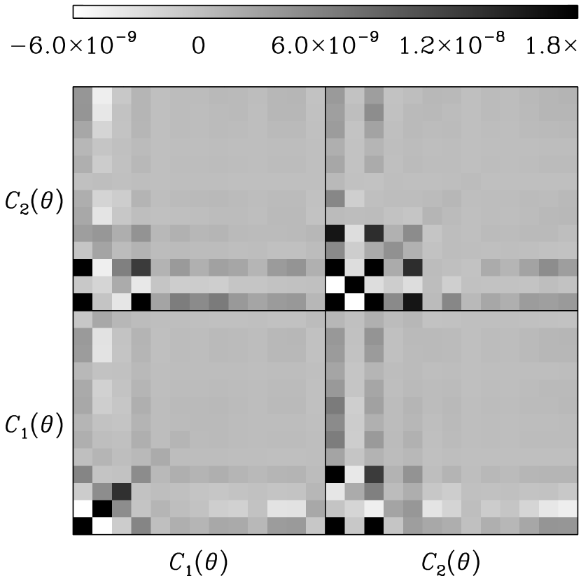
Figure 4: Covariance matrix for the 2D correlation functions $C_{1}(\theta)$ and $C_{2}(\theta)$ shown in figure 2, obtained by splitting the COSMOS field into four quadrants and performing the analysis separately in each. The diagonal elements illustrate the size of the errors in each of the thirteen $\theta$ bins, and the off-diagonal elements illustrate how much the measurements are correlated. The color scale is logarithmic.

3.4 2D shear variance

For historical reasons, cosmic shear results are often expressed as the variance of the shear field in circular cells on the sky. For a top-hat cell of radius $\theta$, this measure is related to the shear correlation functions by

$$\sigma_{\gamma}^{2}\equiv\langle~{}|\overline{\gamma}|^{2}\rangle\approx\frac{2}{\theta^{2}}\int_{0}^{\theta}\Big{[}C_{1}(\vartheta)+C_{2}(\vartheta)\Big{]}~{}{\rm d}\vartheta~{},$$ (12)

where we have used a small angle approximation. Note that the signal is more strongly correlated on different angular scales in this form than it is when expressed as correlation functions. The results are shown in figure 5.

Figure 5: Variance of the 2D shear signal in circular cells of varying size. Solid lines show predictions in a concordance cosmology with $\sigma_{8}$ varying as in figure 2. Note that adjacent data points are highly correlated.

3.5 2D E-B decomposition

The correlation functions can also be recast in terms of non-local $E$ (gradient) and $B$ (curl) patterns in the shear field (Crittenden et al., 2000; Pen et al., 2002). Gravitational lensing is expected to produce only $E$ modes, except for a very low level of $B$ modes due to lens-lens coupling along a line of sight (Schneider et al., 2002). It is commonly assumed that systematic effects would affect both $E$- and $B$-modes equally. The presence of a non-zero $B$ mode is therefore a useful indication of contamination from other sources.

Figure 6: $E$-$B$ decompositions of the 2D shear field. The top panel shows the statistics that formally require an integral over the measured correlation functions to infinite scales, and the bottom panel shows those that formally require an integral from zero. Solid points show the $E$-mode, and open points show the $B$-mode. The lines show predictions in a concordance cosmology with $\sigma_{8}$ varying as in figure 2. Note that adjacent data points are in the top panel are highly correlated.

$E$- and $B$-modes correspond to patterns within an extended region on the sky, and cannot be separated locally. As a result, this operation formally requires an integration of the shear correlation functions over a wide range of angular scales. Two mathematical functions have been developed (Crittenden et al., 2000; Schneider et al., 2002), which each include an integral over only small scales or large scales (see Schneider & Kilbinger (2006) for a new suggestion to construct a third). However, neither integral is ideal in practice, because our correlation functions are only well measured on scales between $\sim 0.5\arcmin$ and $40\arcmin$. The absence of complete data introduces an unknown constant of integration, and it is not possible to uniquely split this measured shear field into distinct $E$- and $B$-mode components. As a practical attempt to estimate this constant, we extrapolate data into the unknown régime, using predictions from the best-fit cosmology that is determined in §5.

The signal on large angular scales is small, and the corresponding integrals require the least correction. To calculate these, we first define $C_{+}\equiv C_{1}+C_{2}$ and $C_{-}\equiv C_{1}-C_{2}$. Then we can compute

$$\xi_{E}(\theta)\equiv C_{1}(\theta)+2\int_{\theta}^{\infty}\left(1-\frac{3\theta^{2}}{\vartheta^{2}}\right)\frac{C_{-}(\vartheta)}{\vartheta}~{}{\rm d}\vartheta~{},$$ (13)

which contains only the $E$-mode signal and

$$\xi_{B}(\theta)\equiv C_{2}(\theta)-2\int_{\theta}^{\infty}\left(1-\frac{3\theta^{2}}{\vartheta^{2}}\right)\frac{C_{-}(\vartheta)}{\vartheta}~{}{\rm d}\vartheta~{},$$ (14)

which contains only the $B$-mode signal. It is generally necessary to add a function of $\theta$ (not only a constant of integration) to $\xi_{E}(\theta)$ and subtract it from $\xi_{B}(\theta)$ (c.f. Pen et al., 2002).

The components can also be separated via the variance of the aperture mass statistic $M_{\rm ap}(\theta)$. This is obtained from a weighted mean of the tangential ($\gamma_{t}$) and radial ($\gamma_{r}$) components of shear relative to the center of a circular aperture. This statistic is given by

$$M_{\rm ap}(\theta)\equiv\int_{0}^{\infty}~{}W\left(|\vec{\vartheta}|;\theta\right)~{}\gamma_{t}\left(\vec{\vartheta}\right)~{}{\rm d}^{2}\vec{\vartheta}$$ (15)

which contains only contributions from the $E$-mode signal and

$$M_{\perp}(\theta)\equiv\int_{0}^{\infty}~{}W\left(|\vec{\vartheta}|;\theta\right)~{}\gamma_{r}\left(\vec{\vartheta}\right)~{}{\rm d}^{2}\vec{\vartheta}~{},$$ (16)

which contains only the $B$-mode signal, where $W(|\vec{\vartheta}|)$ is a compensated filter. We adopt a compensated “Mexican hat” weight function

$$W(\vartheta;\theta)=\frac{6}{\pi\theta^{2}}\frac{\vartheta^{2}}{\theta^{2}}\left(1-\frac{\vartheta^{2}}{\theta^{2}}\right){\rm H}(\theta-\vartheta)~{},$$ (17)

where $\theta$ defines an angular scale of the aperture and the Heaviside step function ${\rm H}$ truncates the weight function on large scales.

Schneider et al. (2002) derived expressions for the variance of these statistics as the aperture is moved across the sky. These reqire integrals over the correlation functions from small scales

$$\left\langle M^{2}_{\rm ap}\right\rangle(\theta)\equiv\frac{1}{2}\int_{0}^{2\theta}\frac{\vartheta}{\theta^{2}}\Bigg{[}C_{+}(\vartheta)T_{+}\left(\frac{\vartheta}{\theta}\right)~{}~{}~{}~{}~{}~{}~{}~{}$$

$$+~{}C_{-}(\vartheta)T_{-}\left(\frac{\vartheta}{\theta}\right)\Bigg{]}~{}{\rm d}\vartheta~{}$$ (18)

$$\left\langle M^{2}_{\perp}\right\rangle(\theta)\equiv\frac{1}{2}\int_{0}^{2\theta}\frac{\vartheta}{\theta^{2}}\Bigg{[}C_{+}(\vartheta)T_{+}\left(\frac{\vartheta}{\theta}\right)~{}~{}~{}~{}~{}~{}~{}~{}$$

$$-~{}C_{-}(\vartheta)T_{-}\left(\frac{\vartheta}{\theta}\right)\Bigg{]}~{}{\rm d}\vartheta,$$ (19)

where

$$T_{+}(x)~{}=~{}\frac{6(2-15x^{2})}{5}\left[1-\frac{2}{\pi}\arcsin\left(\frac{x}{2}\right)\right]~{}+~{}~{}~{}~{}~{}$$ (20)

$$\frac{x\sqrt{4-x^{2}}}{100\pi}\big{(}120+2320x^{2}-754x^{4}+132x^{6}-9x^{8}\big{)}$$

$$T_{-}(x)~{}=~{}\frac{192}{35\pi}x^{3}\left(1-\frac{x^{2}}{4}\right)^{7/2}~{}~{}~{}~{}~{}~{}~{}~{}~{}~{}~{}~{}~{}~{}~{}~{}~{}~{}~{}~{}$$ (21)

for $x<2$ and $T_{+}(x)=T_{-}(x)=0$ for $x\geq 2$. We again estimate the constant of integration by extrapolating our data with theoretical predictions in cosmological model preferred by the rest of the data.

From figure 6, we can see that $\xi_{B}(\theta)$ is consistent with zero on all scales. The noise is particularly large on small scales, and the rather unstable $M^{2}_{\perp}(\theta)$ is affected on scales up to $\sim 1\arcmin$ by the first bin.

4 3D shear analysis

Figure 7: The thin, solid line shows the redshift distribution of source galaxies. The thick, solid line shows their distribution after accounting for the magnitude-dependent weighting scheme. In both cases, the bin size is $\Delta z=0.02$. The dashed lines show (artificially normalized) redshift sensitivity curves obtained by slicing this distribution into the discrete redshift bins indicated by the arrows at the top.

4.1 Correlation function tomography

We now split the catalog into three discrete redshift bins and, as before, calculate the correlation functions using all pairs of galaxies within each bin. The redshift bins are chosen in consideration of the particular color information available. Degeneracies in the photometric redshift estimation cause galaxies with a flat distribution in redshift to cluster artificially around $z=1.3$, 1.6 and 2.2. An excess at these positions is evident in figure 1. We therefore pick bins with boundaries away from these values, and with widths similar to the size of the local peaks in the resdshift distribution. For COSMOS, suitable bins are $0.1\leqslant z\leqslant 1$, $1<z\leqslant 1.4$ and $1.4<z\leqslant 3$. This scheme conveniently divides up the galaxies fairly evenly, with the slices each containing $32\%$, $24\%$ and $44\%$ of the galaxies. Unfortunately, the last bin can not be further sub-divided without deeper IR or UV data. The redshift slices and their resulting lensing sensitivity functions are illustrated in figure 7.

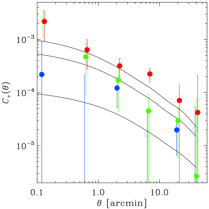
Figure 8: Evolution of the cosmic shear two-point correlation function signal with increasing redshift. The series of data points, from bottom to top, show measurements from slices between redshifts 0.1, 1, 1.4, and 3. The black curves show predictions from a flat $\Lambda$CDM model with $\Omega_{\rm m}=0.3$ and $\sigma_{8}=0.85$, for the same slices, increasing in redshift from the bottom to the top. Open circles depict negative values.

Figure 8 shows the increasing two point correlation function signal for pairs of source galaxies as a function of redshift, where both galaxies are in the same redshift bin. Since the measurements in the redshift bins are much more noisy than those from the projected 2D analysis, we plot $C_{+}(\theta)\equiv C_{1}(\theta)+C_{2}(\theta)$ in figure 8. Theoretical predictions for the correlation functions are obtained for each slice by replacing the lensing weight function $g(z)$ in equation (6) by those shown in figure 7, and obtained from only the galaxies in a given slice. Because the effective lensing volume $\int g(z)~{}{\rm d}z$ increases for succesive redshift bins, the signal increases with $z$.

Figure 9 shows the measured covariance matrix for the 3D correlation functions. The degree of correlation between the lowest and highest redshift bins, primarily evident on small scales, is unexpected. Had it been significant on all scales, a likely explanation would have been cross-contamination of the bins by galaxies from other redshifts (the well-known degeneracy between low and high redshift from photo-$z$ estimation is discussed in §2.4). Had the covariance been equally evident in all three bins, likely explanations could have been: interference of intrinsic alignments like those suggested by (Hirata & Seljak, 2004); and imperfect correction for PSF variation or DRIZZLE-related pixellisation effects unaccounted for on small scales. In practice, the most likely explanation is a combination of several such effects, each at a low level.

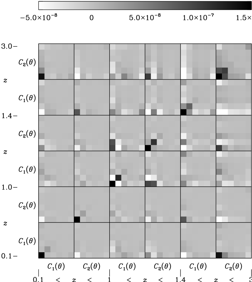
Figure 9: Covariance matrix of correlation function data used in the 3D cosmic shear analysis. Note that this includes only the three correlation functions where both galaxies are in the same redshift bin. An additional three correlation functions can be formed from pairs in which the galaxies come from different slices, but these are not shown in this plot for the sake of clarity.

Although the signal in the individual slices is noisy, we have attempted an $E$-$B$ decomposition in figure 10, using the same two statistics as were applied to the 2D analysis. The integrals over the noisy correlation functions are particularly ill-defined at $\theta<1\arcmin$. Nevertheless, the signal increases to high redshift, matching the theoretical expectation for this measurement.

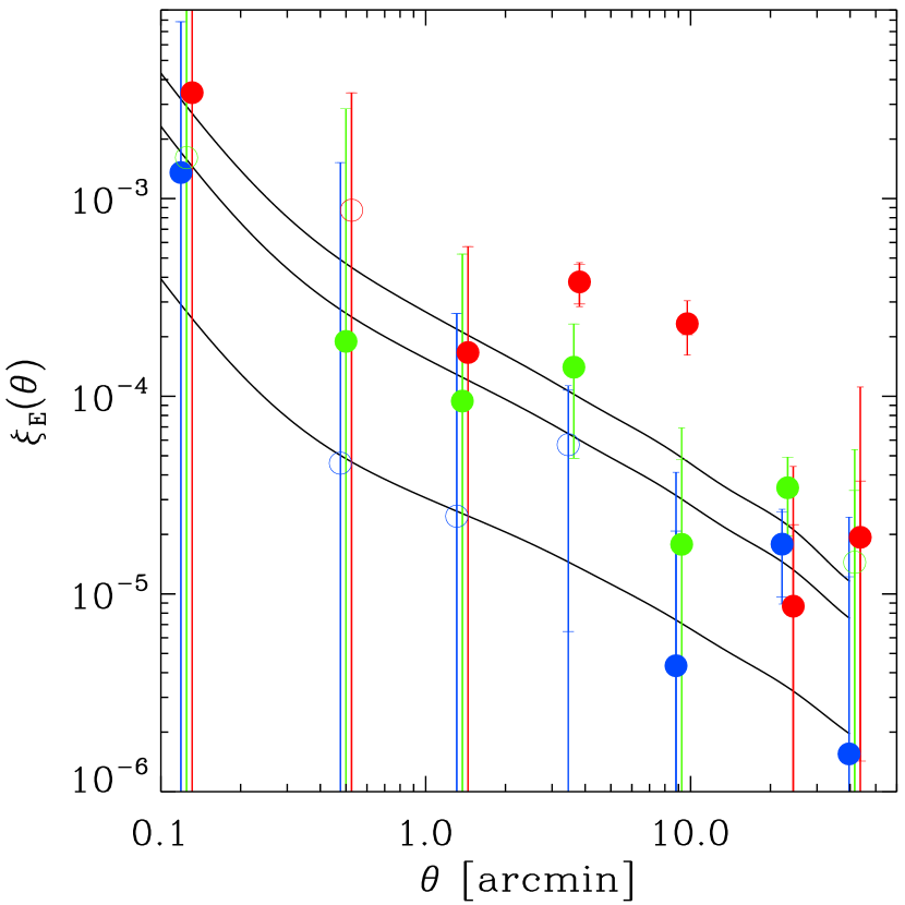
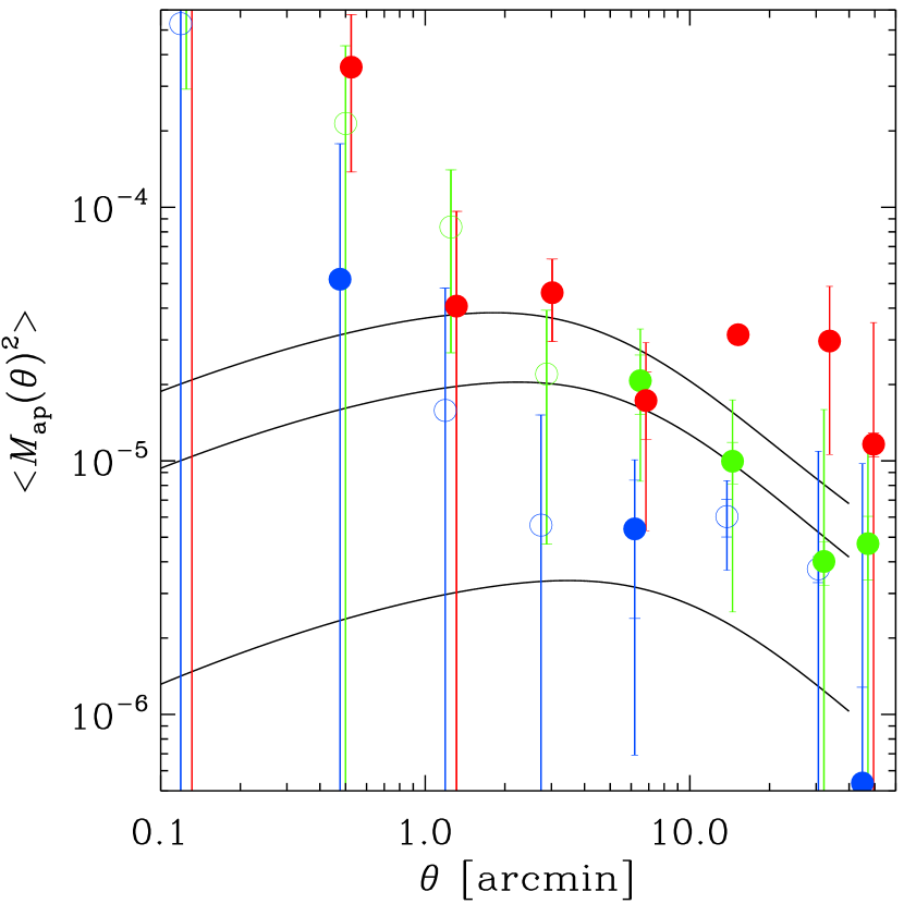
Figure 10: $E$-$B$ decomposition of the 3D cosmic shear signal, in different redshift bins, colored as in figure 8. For clarity, only the $E$-modes are shown. Open circles depict negative values. The $B$-modes are as noisy, but are consistent with zero. Note that adjacent data points are highly correlated.

4.2 Growth of structure

The total $E$-mode signal corresponds to the integrated mass density along a line of sight, weighted by the lensing sensitivity function. The evolving $E$-mode signal in figures 8 and 10 grows towards high redshift due to the increasing volume that it probes, and in which mass structures are located. This offers constraints on the large-scale geometry of the universe. But, if we are more interested in the mass structures themselves, this function of $\theta$ in fixed redshift slices can be recast into a function of $z$ for fixed angular scales. We shall now suggest a new way of viewing this data, which stays close to measurable quantities, but offers a new insight into the underlying structure formation.

Each data point in figure 8 corresponds to the amount of mass within an effective volume. This volume is described in azimuthal directions by Bessel functions, and in the redshift direction by the lensing sensitivity function $g(z)$. Assuming the best-fit cosmology from §5 to fix the geometry of the universe, we can divide by this volume, and obtain a quantity proportional to mass density. In practice, to increase the signal-to-noise of a measurement that will involve many redshift bins, we do not restrict the measurement to only those pairs within a given redshift slice, as before. We require the nearer galaxy to be inside the slice, but then compute correlation functions using all galaxies behind it. The more distant galaxy has then been lensed by anything the foreground has been lensed by. The effect is merely to change the (squared) lensing sensitivity function to the product of the sensitivity function for the slice galaxies with that of the background distribution. This creates a new, effective $g(z)$ that peaks at slightly higher redshift, but is still zero behind the nearest galaxy.

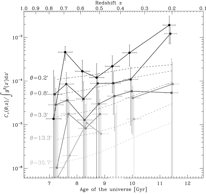
Figure 11: The growth of structure over cosmic time. This links the cosmic shear signal on fixed angular scales as a function of redshift (rather than the other way round, as in previous figures). Data points are located at the peak of the lensing sensitivity function for each set of source galaxies. The source galaxies themselves are approximately twice as far away. The different colors distinguish different angular scales. For each of these, the dashed line shows the theoretical expectation, assuming the best-fit cosmological model from §5.

Figure 11 thus shows

$$G(z;\theta) \equiv C_{+}(\theta;z)~{}\Big{/}\int_{0}^{z}g^{2}(z^{\prime})~{}{\rm d}z^{\prime}$$ (22)

$$= \frac{1}{2\pi}\frac{\int C_{\ell}^{\gamma}(\theta;z)~{}J_{0}(\ell\theta)~{}\ell{\rm d}\ell}{\int_{0}^{z}g^{2}(z^{\prime})~{}{\rm d}z^{\prime}}~{},$$ (23)

the growth of power on different angular scales. The foreground mass is most likely to lie near the peak of the sensitivity function, so we place the data points at this redshift. In practice, it could lie anywhere within $g(z)$, so we overlay error bars in $z$ equal to the rms of $g$ about its peak. Theoretical predictions of this quantity are overlaid, assuming a flat, $\Lambda$CDM cosmology, with the best-fit parameters found in §5.

The growth towards $z=0$ represents a combination of the physical growth of structure and the mixing of fixed physical scales at different redshifts into a measurement at one apparent angular scale. Both of these effects act in the same sense, to increase the signal towards the present day. This is in contrast to the cosmic shear signal in figures 8 and 10, which itself increases towards high redshift. On large scales, the small cosmic shear signal makes the measurement fairly noisy. On intermediate scales, the data closely follow the predictions. The lowest redshift point is obtained from pairs of galaxies where the nearest is between $z=0.1$ and $z=0.7$. We speculate that the apparently significant upturn at low $z$ and on small scales might be caused by contamination of that redshift bin by high redshift galaxies. These could have been caught by the photometric redshift degeneracy discussed in §2.4 and would contain a apparently spurious signal when moved to low redshift. The accuracy of the photometric redshifts may therefore be limiting the precision of this measurement.

5 Constraints on cosmological parameters

5.1 2D parameter constraints

We now use a Maximum Likelihood method to determine the constraints set by our 2D observations of $C_{1}(\theta)$ and $C_{2}(\theta)$ upon the cosmological parameters $\Omega_{\rm m}$, the total mass-density of the universe, and $\sigma_{8}$, the normalization of the matter power spectrum at 8 $h^{-1}$ Mpc. We assume a flat universe, with a Hubble parameter $h=0.7$.

We closely follow the approach of Massey et al. (2005), obtaining theoretical predictions for the linear transfer function from the fitting functions of Bardeen et al. (1986) and for the non-linear power spectrum using the fitting functions of Smith et al. (2003). The theoretical correlation functions are first calculated from equation (6) in a three dimensional grid spanning variations in $\Omega_{\rm m}$ from 0.05 to 1.1, $\sigma_{8}$ from 0.35 to 1.4 and the power spectrum shape parameter $\Gamma$ from 0.13 to 0.33. We used the full redshift distribution of source galaxies (after correction for weighting) shown in figure 1.

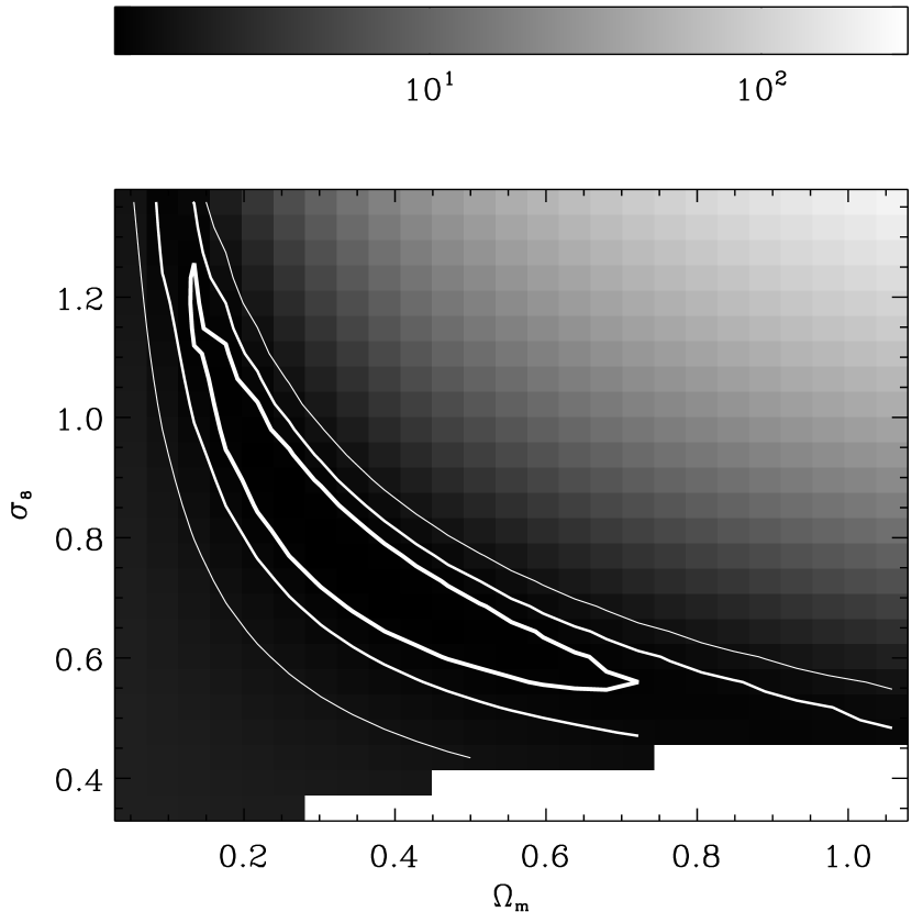
Figure 12: Constraints on cosmological parameters from a traditional 2D cosmic shear analysis, after marginalization over other free parameters. In order of decreasing thickness, the contours indicate $68.3\%$, $95.4\%$ and $99.7\%$ confidence limits due to statistical errors; additional uncertainty potentially contributed by sources of systematic error are discussed in the text. The grey scale background is logarithmic, and shows $\chi^{2}$ divided by the number of degrees of freedom in the data. The white area at the bottom-right was excluded because the Smith et al. (2003) fitting functions could not be evaluated without unreasonable extrapolation of the non-linear matter power spectrum to physical scales smaller than $0.1h^{-1}$kpc. This can be compared to the much tighter constraints from the full 3D analysis in figure 15.

We then fitted the observed shear correlation functions $\vec{d}(\theta)=\{C_{1}(\theta),C_{2}(\theta)\}$ to the theoretical predictions calculated at the centers of each bin $\vec{t}(\theta)$, computing the log-likelihood function

$$\chi^{2}(\vartheta,\Omega_{\rm m},\sigma_{8},\Gamma)=\big{(}\vec{d}(\theta)-\vec{t}(\theta,\Omega_{\rm m},\sigma_{8},\Gamma)\big{)}^{T}~{}{\rm cov}(d)^{-1}~{}\big{(}\vec{d}(\vartheta)-\vec{t}(\vartheta,\Omega_{\rm m},\sigma_{8},\Gamma)\big{)}$$

throughout the grid, where ${\rm cov}(d)$ is the covariance matrix in figure 4. In an advance of earlier incarnations, we perform the matrix inversion via a singular value decomposition (SVD), and discard all eigenvalues not within machine precision of the largest. We do not include the multiplicative factor suggested by Hartlap, Simon & Schneider (2007). We then marginalize over $\Gamma$ with a Gaussian prior centered on 0.19 and with an rms width of 15% (Percival et al., 2001). To compute confidence contours, we numerically integrate the likelihood function

$$L(\Omega_{\rm m},\sigma_{8})~{}=~{}e^{-\chi^{2}/2}~{}.$$ (24)

Our constraints on cosmological parameters from this 2D analysis are presented as a projection through parameter space in figure 12. The contours represent statistical errors, including full non-Gaussian sample variance. Formally, the best-fit model has $\Omega_{m}=0.30$, $\sigma_{8}=0.81$ and $\Gamma=0.21$, and this achieves $\chi^{2}_{\rm reduced}\equiv\chi^{2}/(n_{\rm param}-3)=1.10$ in 23 degrees of freedom. However, there is a well-known degeneracy between $\Omega_{\rm m}$ and $\sigma_{8}$ when using only two-point statistics. Changing the $\Gamma$ parameter slides the contours back and forth along this valley, and marginalization over this parameter also slightly increases the minimum $\chi^{2}$. After marginalization, a good fit to our 68.3% confidence level from statistical errors is given by

$$\sigma_{8}\left(\frac{\Omega_{m}}{0.3}\right)^{0.44}=0.81\pm 0.075~{},$$ (25)

with $0.15\leqslant\Omega_{\rm m}\leqslant 0.7$.

Massey et al. (2005) were unable to use the full covariance matrix due to instabilities in the matrix inversion, so had set to zero any elements in the covariance of $C_{1}(\theta)$ with $C_{2}(\theta)$ (these are the bottom-left and top-right quarters in figure 4). This problem has been resolved in the present work by the use of an SVD. However, if we discard half of the covariance matrix as in Massey et al. (2005), we obtain parameter constraints

$$\sigma_{8}\left(\frac{\Omega_{m}}{0.3}\right)^{0.44}=0.83\pm 0.07~{}.$$ (26)

If we discard all of the off-diagonal elements in the covariance matrix, we obtain

$$\sigma_{8}\left(\frac{\Omega_{m}}{0.3}\right)^{0.44}=0.84\pm 0.065~{}.$$ (27)

The slightly smaller error bars are expected, but the shift in the best-fit value relative to result (25) is not. This effect might go some way towards explaining the higher than usual value obtained for this quantity in Massey et al. (2005).

Note that all of the above constraints incorporate only statistical sources of error; although these do include non-Gaussian sample variance and marginalization over other parameters. We can propagate the various sources of potential systematic error by noting that

$$C_{i}(5^{\prime})\propto\Omega_{\rm m}^{1.46}\sigma_{8}^{2.45}z_{s}^{1.65}\Gamma^{-0.11}(P^{\gamma})^{-2},$$ (28)

for $i\in\{1,2\}$ in a fiducial $\Lambda$CDM cosmological model with $\Omega_{\rm m}=0.3$, $\Omega_{\Lambda}$=0.7, $\Gamma=0.21$ and $\sigma_{8}=1.0$. Adding an uncertainty equivalent to 10% in the median source redshift, a 6% shear calibration uncertainty (see Leauthaud et al., 2007; Heymans et al., 2006; Massey et al., 2007), and an empirically estimated binning instability (c.f. Massey et al., 2005) to our constraint from the full covariance matrix gives a final 68.3% confidence limit of

$$\sigma_{8}\left(\frac{\Omega_{m}}{0.3}\right)^{0.48} = 0.81\pm 0.075\pm 0.024\pm 0.05\pm 0.02$$ (29)

$$= 0.81\pm 0.17~{},$$

where the various systematic errors have been combined linearly on the second line.

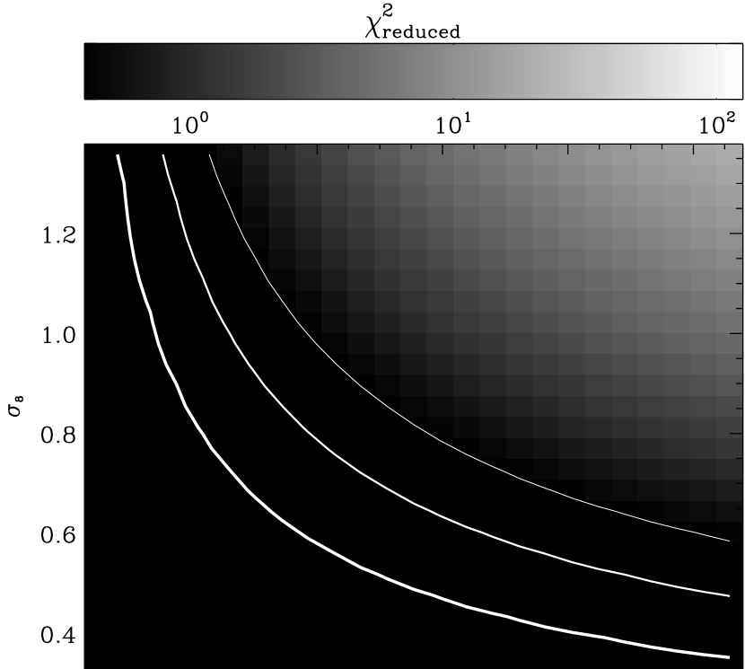
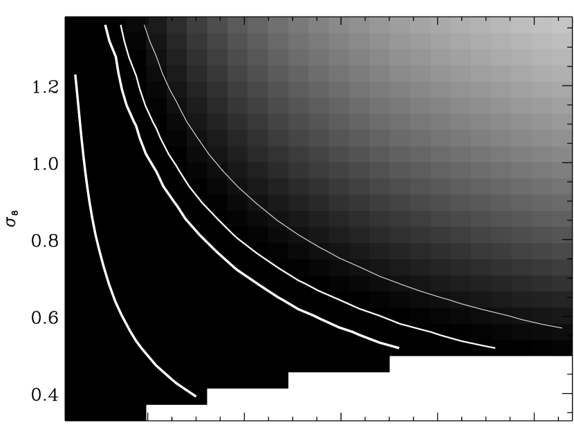
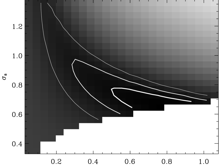
Figure 13: Constraints on cosmological parameters from within each of the three separate redshift slices, from low (top panel) to high redshift (bottom panel). The redshift binning scheme is shown in figure 7 and discussed in the text. The contours indicate $68.3\%$, $95.4\%$ and $99.7\%$ confidence limits, and the logarithmic color scale is common to all three slices.

5.2 3D parameter constraints

We shall now include the redshift information available for each object, adopting the 3D binning scheme introduced in §4. A simple 2D analysis can first be performed within each redshift slice, by simply exchanging the redshift sensitivity function $g(z)$ calculated using the full redshift distribution for one calculated using the restricted distributions. Figure 13 shows the constraints on cosmological parameters from each slice, using only pairs of galaxies where both pairs lie in that slice, but the full covariance matrix for each. The individual results are clearly more noisy than for the full 2D analysis, since each slice contains only approximately one ninth of the number of galaxy pairs. However, all of the slices are consistent with our base cosmological model. Furthermore, while the statistical noise is similar in each slice, because they all contain a similar number of galaxy pairs, the signal (and hence the signal to noise) clearly increases at high redshift, as expected.

In figure 14, the constraints from the three redshift bins are combined as if they all provided independent information (despite the fact that the redshift sensitivity functions in figure 7 clearly overlap, so they are correlated). Although there are approximately only one third of the number of galaxy pairs in this analysis as there were in the 2D analysis, the additional information about the evolution of the signal as a function of redshift retightens the 68% confidence limit constraints back to a similar value of

$$\sigma_{8}\left(\frac{\Omega_{m}}{0.3}\right)^{0.44}=0.86\pm 0.08~{},$$ (30)

for $\Omega_{m}\geqslant 0.25$. The best-fit model has $\Omega_{m}=0.55$ and $\sigma_{8}=0.64$, which achieves $\chi^{2}_{\rm reduced}=1.18$ in 28 degrees of freedom.

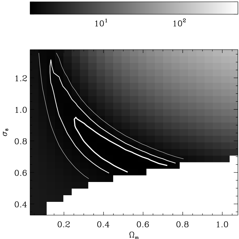
Figure 14: Combined constraints on cosmological parameters $\Omega_{\rm m}$ and $\sigma_{8}$ from a series of effectively 2D shear analyses in each of the three redshift slices (see text). Only pairs of galaxies where both lie in the same redshift slice have been included in this analysis. This can be compared to the similar result from the 2D analysis in figure 12, and the full 3D analysis in figure 15.

We can restore the missing galaxy pairs, and their information content, by introducing three additional correlation functions, constructed from pairs of galaxies that lie in different redshift slices. The theoretical expectation for these correlation functions requires the $g^{2}(z)$ term in equation (6) to be replaced by the product of the lensing sensitivity functions for the two redshift bins. We use the full covariance matrix, which is again estimated from variation between the four quadrants of the COSMOS field. Figure 15 shows a projection of the log-likelihood surface, with the usual contours.

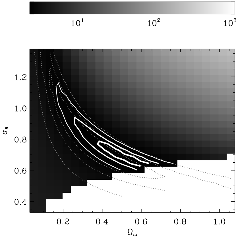
Figure 15: Constraints on cosmological parameters $\Omega_{\rm m}$ and $\sigma_{8}$, from a full 3D cosmic shear analysis. Solid contours indicate $68.3\%$, $95.4\%$ and $99.7\%$ confidence limits due to statistical errors and marginalization over other parameters; potential sources of additional, systematic error are discussed in the text. These constraints are far tighter than the equivalent results from our simple 2D analysis, which are reproduced from figure 12 as dotted lines for ease of comparison. The white area at the bottom-right was excluded because the Smith et al. (2003) fitting functions could not be evaluated without unreasonable extrapolation of the non-linear matter power spectrum to physical scales smaller than $0.1h^{-1}$kpc.

The best-fit model has $\Omega_{m}=0.47$ and $\sigma_{8}=0.72$, which achieves $\chi^{2}_{\rm reduced}=2.35$ in 56 degrees of freedom. This is significantly greater than unity because only statistical errors are currently included. As described below, the error budget is increased by a factor of $\sim 1.5$, and the minimum $\chi^{2}_{\rm reduced}$ to 1.04, when considering systematic errors in the relative shear calibration and mixing of galaxies between bins. Again we find the usual degeneracy, the best-fit position along which is determined by the parameter $\Gamma$. However, with the full 3D information, parameter constraints in the direction orthogonal to this are much tighter. Our 68% confidence limits are well-fit by

$$\sigma_{8}\left(\frac{\Omega_{m}}{0.3}\right)^{0.44}=0.866\pm 0.033~{},$$ (31)

for $0.3\leqslant\Omega_{m}\leqslant 0.6$.

We now incorporate a systematic error budget into our 3D parameter constraints. We allow a 6% absolute shear calibration uncertainty (Leauthaud et al., 2007), a 5% relative shear calibration uncertainty between low and high redshift bins, and a potential 10% contamination (e.g. Massey et al., 2004) of the high redshift bin by galaxies really at low redshift (and vice versa) due to the possibility of catastrophic redshift errors discussed in §2.4. This leaves a final 68.3% confidence limit of

$$\sigma_{8}\left(\frac{\Omega_{m}}{0.3}\right)^{0.44} = 0.866\pm 0.033\pm 0.026\pm 0.009^{+0.017}_{-0.000}$$ (32)

$$= 0.866^{+0.085}_{-0.068}~{},$$

where the various systematic errors have been combined linearly on the second line. Note that, when considering the relative improvement in the parameter constraints from a 2D analysis (29) to a 3D analysis (32), it is not appropriate to include errors from uncertainty in the absolute calibration of a shear measurement method that is common to both. Continuing to budget for potential relative mis-calibration between low- and high-redshift bins, as well as including all other sources of systematic and statistical error, reveals a dramatic threefold tightening of parameter constraints.

We have also tried increasing the number of redshift slices, for a finer quantitative measurement of the evolution of the shear signal. We attempted an analysis using five redshift bins, created by splitting in half the first two slices of the three used previously. Unfortunately, the covariance matrix became degenerate, and harder to invert. Furthermore, the best-fit$\chi^{2}_{\rm reduced}$ and cosmological parameter constraints degraded. The results in each bin were very noisy (the signal to noise is proportional to $n^{-2}_{\rm galaxies}$), but, as in §4.2, there were hints that the signal did not evolve as expected after this finer redshift binning. The likelihood surfaces from individual slices did not agree, so their combination was blurred out. We interpret this as indicating that galaxies were beginning to be placed in the wrong redshift bins, and polluting that signal. Thus we have effectively reached the available precision of the photometric redshifts, at least at the high redshifts in which the weak lensing signal is concentrated. For further progress, we await ongoing, deeper multicolor observations of the COSMOS field.

6 Conclusions

We have performed a fully three dimensional cosmic shear analysis of the largest ever survey with the Hubble Space Telescope. The 3D shear field contains rich information about the growth of structure and the expansion history of the universe. Indeed, by assuming a concordance cosmological model, we have directly measured the growth of structure on both linear and non-linear physical scales. We have also placed independent 68% confidence limits on cosmological parameters. From a traditional, two dimensional cosmic shear analysis, we measure

$$\sigma_{8}\left(\frac{\Omega_{m}}{0.3}\right)^{0.48}=0.81\pm 0.17~{},$$ (33)

with $0.15\leqslant\Omega_{\rm m}\leqslant 0.7$. From a full, three dimensional analysis of the same data, we obtain

$$\sigma_{8}\left(\frac{\Omega_{m}}{0.3}\right)^{0.44}=0.866^{+0.085}_{-0.068}~{},$$ (34)

with $\Omega_{m}\geqslant 0.3$. This represents a dramatic improvement over already remarkable constraints. In fact, disregarding uncertainty in the absolute calibration of our shear measurement method, which is common to both analyses, the 3D constraints represent a threefold relative improvement in the errors from the 2D constraints.

A solely two-point cosmic shear analysis cannot easily isolate a measurement of just $\Omega_{m}$. The degeneracy with $\sigma_{8}$ is broken only by the difference in signal between large and small scales. Our best-fit value of $\Omega_{m}$ is slightly larger than the measurement of $0.23\pm 0.02$ from the 2dF galaxy redshift survey (Cole et al., 2005). As discussed in §3.3, undetected CTE correction residuals could potentially affect our measurement on the very largest scale in each redshift slice; however this datum carries very little weight because of shot noise, so this explanation is unlikely. Because high redshift slices probe larger physical scales than low redshift slices, our measurement of $\Omega_{m}$ could also be potentially biased by photometric redshift failures. After allowing for this effect in our systematic error budget, the discrepancy in $\Omega_{m}$ is within $1\sigma$ of the 2dF results, so we shall not pursue this further.

The main constraint from our data is upon $\sigma_{8}$. We find a value slightly larger than that of $0.74^{+0.05}_{-0.06}$ from the 3-year WMAP data (Spergel et al., 2006). Our result is also larger than most estimates of cluster abundance from $x$-ray surveys (e.g. Borgani et al., 2001; Schneider et al., 2002), and from other recent space-based weak lensing measurements (Heymans et al., 2005; Schrabback et al., 2007). However, the HST GEMS survey, on which both of the latter were based, suffers from sample variance due to its limited size, and is suspected from other measures of containing an unusually empty portion of the universe. Furthermore, independent measurements of $\sigma_{8}=0.85$ or slightly greater have recently been published by McCarthy, Bower & Balogh (2006), from observations of the gas mass fraction in $x$-ray selected clusters; Li et al. (2006), by counting the number of observed giant arcs; and Viel, Haenelt & Springel (2004) and Seljak, Slosar & McDonald (2006), with Lyman-$\alpha$ forest data. All of these measures contain information about small-scale density fluctuations at relatively low redshift: something much more intrinsically suited to a measurement of $\sigma_{8}$ than the CMB. Our results are also remarkably consistent with those from the ground-based CFHT wide synoptic legacy survey (Hoekstra et al., 2006). Such agreement between the largest space-based and ground-based surveys demonstrates the maturity of the field post-STEP. The combination of all these results is therefore beginning to hint at inconsistencies in either the standard cosmological model or in the interpretation of one or more of these methods.

With the profundity of this statement in mind, we are careful to realistically include all possible sources of systematic error. The dominant contribution to the total error budget is uncertainty in the absolute calibration of our shear measurement method. The weak lensing community is earnestly working to improve and ascertain the reliability of various methods through simulated images that contain a known input signal (Leauthaud et al., 2007; Heymans et al., 2006; Massey et al., 2007).

Aside from this contribution, further exploitation of the COSMOS survey is currently limited by two additional sources of potential systematic error. Conveniently, these two limits currently happen to lie at a similar flux level and therefore affect a similar population of galaxies, which we simply remove from our analysis. Since a weak lensing measurement is concerned with the mass distribution in front of galaxies rather than the galaxies themselves, this can be done without worries about bias. Firstly, the in-orbit degradation of the ACS CCDs has led to inadequate charge transfer efficiency during readout, which creates trailing of faint objects, and mimics a weak lensing signal. In Rhodes et al. (2007), we formulated an empirical correction scheme for the CTE effect, which works for all but the faintest galaxies; an ongoing effort to correct CTE pixel-by-pixel in raw images should allow us to push this limit and dramatically increase the number density of galaxies with measured shears. Secondly, the finite number of colors available for each galaxy, and particularly the depth in near-IR bands, limits the current accuracy of photometric redshifts. Continuing observations with the Subaru telescope should improve their precision. This will allow finer resolution in the redshift direction and, most importantly, will break redshift degeneracies ubiquitous in the redshifts of faint objects so that they can also be used.

By understanding the characteristics of effects that dominate real data, COSMOS is proving an invaluable dry run for future, dedicated weak lensing missions in space. We have revealed important aspects that should ideally be minimized by hardware design and mission scheduling requirements. However, we have also demonstrated the rich information content of the 3D shear field, and shown a proof of concept for some of the proposed tomographic analysis techniques that will be required to fully exploit such future data.

References

- Capak et al. (2007) Capak P. et al., 2007, this volume
- Koekemoer et al. (2007) Koekemoer A. et al., 2007, this volume
- Leauthaud et al. (2007) Leauthaud A. et al., 2007, this volume
- Mobasher et al. (2007) Mobasher B. et al., 2007, this volume
- Rhodes et al. (2007) Rhodes J. et al., 2007, this volume
- Scoville et al. (2007a) Scoville N. et al., 2007a, this volume
- Scoville et al. (2007b) Scoville N. et al., 2007b, this volume
- Bacon et al. (2003) Bacon D., Massey R., Refregier A. & Ellis R., 2003, MNRAS, 344, 673
- Bacon, Refregier & Ellis (2000) Bacon D., Refregier A. & Ellis R., 2000, MNRAS, 318, 625
- Bacon et al. (2001) Bacon D., Refregier A., Clowe D. & Ellis R., 2001, MNRAS, 325, 1065
- Bacon et al. (2005) Bacon D. et al. 2005, MNRAS, 363, 723
- Bardeen et al. (1986) Bardeen J., Bond J., Kaiser N. & Szalay A., ApJ, 304, 15
- Bartelmann & Schneider (2000) Bartelmann M. & Schneider P., 2000, Phys. Rep., 340, 291
- Bernstein & Jarvis (2002) Bernstein G. & Jarvis M., 2002, ApJ, 123, 583
- Bernstein & Jain (2004) Bernstein G. & Jain B., 2004, ApJ, 600, 17
- Bertin & Arnouts (1996) Bertin E., Arnouts S., 1996, A&AS, 117, 393
- Borgani et al. (2001) Borgani S., Rosati P., Tozzi P., Stanford S., Eisenhardt P., Lidman C., Holden B., Della Ceca R., Norman C., Squires G., 2001, ApJ, 561, 13.
- Bridle et al. (2001) Bridle S. et al., 2001, in Scientific N. W., Proceedings of the Yale Cosmology Workshop
- Brown et al. (2003) Brown M., Taylor A., Bacon D., Gray M., Dye S., Meisenheimer K. & Wolf C., 2003, MNRAS, 341, 100
- Bristow (2004) Bristow P., 2004, STIS Model-based charge Coupled Device Readout: Simulation Overview and Early Results (CE-STIS-ISR 2002-001; Baltimore, STScI)
- Cole et al. (2005) Cole S. et al., 2005, MNRAS, 362, 505
- Crittenden et al. (2000) Crittenden R., Natarajan P., Pen U.-L. & Theuns T., 2000, ApJ, 559, 552
- Dekel & Lahav (1999) Dekel, A. & Lahav, O., 1999, ApJ, 520, 24
- Erben et al. (2001) Erben T., van Waerbeke L., Bertin E., Mellier Y. & Schneider P., 2001, A&A, 366, 717
- Fruchter & Hook (2002) Fruchter A. & Hook R., 2002, PASP, 114, 144
- Hamana et al. (2003) Hamana T. et al., 2003, ApJ in press (astro-ph/0210450)
- Hartlap, Simon & Schneider (2007) Hartlap J., Simon P. & Schneider P., 2007, A&A in press (astro-ph/0608064)
- Heavens (2005) Heavens A., Kitching T. & Taylor A., 2006, MNRAS submitted (astro-ph/0606568)
- Heymans et al. (2005) Heymans C. et al., 2005, MNRAS, 361, 160
- Heymans et al. (2006) Heymans C. et al., 2006, MNRAS, 371, 750
- Heymans et al. (2007) Heymans C., White M., Heavens A., Vale C. & Van Waerbeke L., 2007, MNRAS in press (astro-ph/0604001)
- Hirata & Seljak (2004) Hirata C. & Seljak U., 2004, Phys. Rev. D, 70, 63526
- Huterer & White (2003) Huterer & White, 2003, ApJ, 578, L95
- Hoekstra et al. (2002b) Hoekstra H., van Waerbeke L., Gladders M., Mellier Y. & Yee H., 2002b, ApJ, 577, 604
- Hoekstra et al. (2006) Hoekstra H., Mellier Y., van Waerbeke L., Semboloni E., Fu L., Hudson M., Parker L., Tereno I. & Benabed K., 2006, ApJ, 647, 116
- Jarvis et al. (2003) Jarvis M., Bernstein G., Fisher P., Smith D., Jain B. et al., 2003, AJ, 125, 1014
- Jarvis & Jain (2005) Jarvis M. & Jain B., 2005, ApJ submitted (astro-ph/0412234)
- Jee et al. (2005) Jee M., White R., Ben tez N., Ford H., Blakeslee J., Rosati P., Demarco R. & Illingworth G., 2005, ApJ, 618, 46
- Kaiser, Squires & Broadhurst (1995) Kaiser N., Squires G. & Broadhurst T., 1995, ApJ, 449, 460
- Kaiser et al. (2000) Kaiser N., Wilson G., & Luppino G. 2000, ApJ submitted (astro-ph/0003338)
- Krist (2003) Krist J., 2003, Instrument Science Rep. ACS 2003-06 (Baltimore: STScI)
- Kuijken (2006) Kuijken K., A&A in press (astro-ph/0601011)
- Li et al. (2006) Li G., Mao S., Jing Y., Mo H., Gao L. & Lin W., 2006, MNRAS in press (astro-ph/0608192)
- Lombardi et al. (2005) Lombardi, M., et al. 2005, ApJ, 623, 42
- McCarthy, Bower & Balogh (2006) McCarthy I., Bower R. & Balogh M, 2006, MNRAS submitted (astro-ph/0609314)
- Mandelbaum et al. (2005) Mandelbaum R., Hirata C. M., Seljak U., Guzik J., Padmanabhan N., Blake C., Blanton M., Lupton R., Brinkmann J., 2005, MNRAS, 361, 1287
- Massey et al. (2004) Massey R. et al., 2004, AJ, 127, 3089
- Massey & Refregier (2005) Massey R. & Refregier A., 2005, MNRAS, 363, 197
- Massey et al. (2004) Massey R., Refregier A., Conselice C. & Bacon D., 2004, MNRAS, 348, 214
- Massey et al. (2005) Massey R., Refregier A., Bacon D., Ellis R. & Brown M., 2005, MNRAS, 359, 1277
- Massey et al. (2007) Massey R. et al., 2007, MNRAS in press (astro-ph/0608643)
- Massey et al. (2006) Massey R., Rowe B., Refregier A., Bacon D. & Bergé J., 2006, MNRAS submitted
- Nakajima & Bernstein (2006) Nakajima R. & Bernstein G., 2006, AJ submitted (astro-ph/0607062)
- Pen et al. (2002) Pen U., Van Waerbeke L. & Mellier Y., 2002, ApJ, 567, 31
- Percival et al. (2001) Percival W. et al. 2001, MNRAS, 327, 1297
- Pierpaoli, Scott & White (2001) Pierpaoli E., Scott D. & White M., 2001, MNRAS, 325, 77
- Refregier (2004) Refregier A., 2004, ARA&A, 41, 645
- Refregier & Bacon (2003) Refregier A. & Bacon D., 2003, MNRAS, 338, 48
- Refregier Rhodes, & Groth (2002) Refregier A., Rhodes, J. & Groth E., 2002, ApJ, 572, 131
- Rhodes, Refregier & Groth (2000) Rhodes J., Refregier A., Groth E., 2000, ApJ, 536, 79
- Rhodes, Refregier & Groth (2001) Rhodes J., Refregier A. & Groth E., 2001, ApJ, 552, 85
- Rhodes et al. (2004) Rhodes J., Refregier A., Collins N., Gardner J., Groth E. & Hill R., 2004, ApJ in press (astro-ph/0312283)
- Seljak, Slosar & McDonald (2006) Seljak U., Slosar A. & McDonald P., 2006, MNRAS submittted (astro-ph/0604335)
- Semboloni et al. (2006) Semboloni E., Mellier Y., van Waerbeke L., Hoekstra H., Tereno I., Benabed K., Gwyn S., Fu L., Hudson M., Maoli R. & Parker L., 2006 A&A, 452, 51
- Semboloni et al. (2006) Semboloni E., van Waerbeke L., Heymans C., Hamana T., Colombi S., White M. & Mellier Y., 2006, MNRAS submitted (astro-ph/0606648)
- Schneider et al. (2002) Schneider P., van Waerbeke, L. & Mellier Y., 2002, A&A, 389, 729
- Schneider & Kilbinger (2006) Schneider P. & Kilbinger M, 2006, A&A submitted (astro-ph/0605084)
- Schrabback et al. (2007) Schrabback, T. et al. 2007, A&A submitted (astro-ph/0606611)
- Schneider et al. (2002) Schuecker P., Bohringer H., Collins C., et al. 2003, A&A, 396, 867
- Smail et al. (1994) Smail I., Ellis R. & Fitchett M., 1994, MNRAS, 270, 245
- Smith et al. (2003) Smith G., Edge A., Eke V., Nichol R., Smail I. & Kneib J.-P., 2003, AJ, 590, L79
- Smith et al. (2003) Smith R., Peacock J., Jenkins A., White S., Frenk C., Pearce F., Thomas P., Efstathiou G. & Couchmann H., 2003, MNRAS, 341, 1311
- Spergel et al. (2006) Spergel D., et al., 2006, ApJ submitted (astro-ph/0603449)
- Taylor (2002) Taylor A., 2002, Phys. Rev. Lett., submitted (astro-ph/0111605)
- Taylor et al. (2006) Taylor A., Kitching T., Bacon D. & Heavens A., MNRAS submitted (astro-ph/0606416)
- Van Waerbeke et al. (2000) van Waerbeke L. et al., 2000, A&A, 358, 30
- Van Waerbeke, Mellier & Hoekstra (2005) van Waerbeke L., Mellier Y. & Hoekstra H., 2005, A&A submitted (astro-ph/0406468)
- Viana, Nichol & Liddle (2002) Viana P., Nichol R. & Liddle A., 2002, ApJ, 569,75
- Viel, Haenelt & Springel (2004) Viel M., Haenelt M. & Springel V., 2004, MNRAS, 354, 684
- Weinberg et al. (2000) Weinberg D., Davé R., Katz N. & Hernquist L., 2003, ApJ submitted (astro-ph/0212356)
- White (2002) White M., 2002, ApJS 143, 241
- Wittman et al. (2000) Wittman D., Tyson J., Kirkman D., Dell’Antonio I., Bernstein G., 2000, Nature, 405, 143
- Wittman (2002) Wittman D. 2002. Dark Matter and Gravitational Lensing, LNP Top. Vol., eds. F. Courbin, D. Minniti. Springer-Verlag (astro-ph/0208063)
- Wittman (2005) Wittman D., 2005, ApJL, 632, 5