Non-blind catalogue of extragalactic point sources from
the Wilkinson Microwave Anisotropy Probe (WMAP)
first 3–year survey data

Abstract

We have used the MHW2 filter to obtain estimates of the flux densities at the WMAP frequencies of a complete sample of 2491 sources, mostly brighter than 500 mJy at 5 GHz, distributed over the whole sky excluding a strip around the Galactic equator ($|b|\leq 5^{\circ}$). After having detected 933 sources at the $\geq 3\sigma$ level in the MHW2 filtered maps - our New Extragalactic WMAP Point Source (NEWPS)_3σ Catalogue - we are left with 381 sources at $\geq 5\sigma$ in at least one WMAP channel, 369 of which constitute our NEWPS_5σ catalogue. It is remarkable to note that 98 (i.e. 26%) sources detected at $\geq 5\sigma$ are ‘new”, they are not present in the WMAP catalogue. Source fluxes have been corrected for the Eddington bias. Our flux density estimates before such correction are generally in good agreement with the WMAP ones at 23 GHz. At higher frequencies WMAP fluxes tend to be slightly higher than ours, probably because WMAP estimates neglect the deviations of the point spread function from a Gaussian shape. On the whole, above the estimated completeness limit of 1.1 Jy at 23 GHz we detected 43 sources missed by the blind method adopted by the WMAP team. On the other hand, our low-frequency selection threshold left out 25 WMAP sources, only 12 of which, however, are $\geq 5\sigma$ detections and only 3 have $S_{23\rm GHz}\geq 1.1\,$Jy. Thus, our approach proved to be competitive with, and complementary to the WMAP one.

1. Introduction

As a by-product of its temperature and polarization maps of the Cosmic Microwave Background (CMB), the Wilkinson Microwave Anisotropy Probe (WMAP) mission has produced the first all-sky surveys of extragalactic sources at 23, 33, 41, 61 and 94 GHz (Bennett et al. 2003; Hinshaw et al. 2006), a still unexplored frequency region where many interesting astrophysical phenomena are expected to show up (see e.g. De Zotti et al. 2005).

¿From the analysis of the first three years survey data the WMAP team has obtained a catalogue of 323 extragalactic point sources (EPS; Hinshaw et al. 2006), substantially enlarging the first-year one that included 208 EPS detected above a flux limit of $\sim 0.8$-1 Jy (Bennett et al., 2003).

As discussed by Hinshaw et al. (2006), the detection process – quite similar to the one adopted for producing the first-year catalogue – can be summarized as follows. First, the weighted map, $N_{obs}^{1/2}T$, where $N_{obs}$ is the number of observations per pixel, is filtered in the harmonic space by the global matched filter,

$$\frac{b_{\ell}}{b^{2}_{\ell}C_{\ell}^{\rm cmb}+C_{\ell}^{\rm noise}},$$ (1)

where $b_{\ell}$ is the transfer function of the WMAP beam response (Page et al., 2003; Jarosik et al., 2006), $C_{\ell}^{\rm cmb}$ is the angular power spectrum of the CMB and $C_{\ell}^{\rm noise}$ represents the noise power. Then, all the peaks above the $5\sigma$ threshold in the filtered maps are assumed to be source detections and are fitted in real space, i.e. in the unfiltered maps, to a Gaussian profile plus a planar baseline. The Gaussian amplitude is finally converted to a flux density using the conversion factors given in Table 5 of Page et al. (2003). The error on the flux density is given by the statistical error of the fit.

If a source has been detected above $5\sigma$, $\sigma$ being the noise rms defined globally, in a frequency channel, the flux densities in the other channels are given if they are above $2\sigma$ and the source width falls within a factor of two of the true beam width. In other words, not all sources listed at any given frequency in the three-year WMAP catalogue of EPS (Hinshaw et al., 2006, Table 9) are $5\sigma$ detections at that frequency. Finally, to identify the detected sources with 5 GHz counterparts, they cross-correlated them with the GB6, PMN and Kühr et al. (1981) catalogues.

The fact that almost all sources detected by WMAP were previously catalogued at lower frequencies suggests that a fuller exploitation of the WMAP data can be achieved complementing the blind search already carried out by the WMAP team with a search for WMAP counterparts to sources detected at lower frequencies. The latter approach exploits the knowledge of source positions to extract as much information as possible on their fluxes.

Since point sources, as any other foreground emission, are a nuisance for CMB experiments, these are designed to keep them as low as possible. Thus, if we are interested in point sources, it is of great importance to develop and apply specific and highly efficient detection algorithms. It has been shown that wavelet techniques perform very well this task (Cayón et al., 2000; Vielva et al., 2001a, b, 2003; González-Nuevo et al., 2006; López-Caniego et al., 2006).

In a recent paper (González-Nuevo et al., 2006) some of us have discussed a natural generalization of the (circular) Mexican Hat wavelet on $R^{2}$, obtained by iteratively applying the Laplacian operator to the Gaussian function, which we called the Mexican Hat Wavelet Family (MHWF). We demonstrated that the MHWF performs better than the standard Mexican Hat Wavelet (MHW, Cayón et al., 2000) for the detection of EPS in CMB anisotropy maps. In a subsequent work (López-Caniego et al., 2006) the MHWF has been applied to the detection of compact extragalactic sources in simulated CMB maps. In that work it was shown, in particular, that the second member of the MHWF, called the MHW2, at its optimal scale compares very well with the standard Matched Filter (MF); its performances are very similar to those of the MF and it is much easier to implement and use. We have therefore decided to apply the MHW2 technique to estimate the flux of the EPS in the 3-year WMAP maps for a complete sample of sources selected at lower frequencies.

The outline of the paper is as follows. In Section 2, we introduce the low-frequency selected sample we have used. In Section 3 we present and discuss the tools for detecting the EPS and for estimating their fluxes. In Section 4 we present and describe our final catalogue. In Section 5 we compare our catalogue with the WMAP one. Finally, in Section 6, we summarize our main conclusions.

2. The 5 GHz catalogue

A summary of the multi–steradian surveys that we have used is given in Table 1. The highest frequency for which an almost complete sky coverage has been achieved is $\simeq 5\,$GHz, thanks to the combined 4.85 GHz GB6 and PMN surveys with an angular resolution of $3.5^{\prime}$ and $4.2^{\prime}$, respectively, and a flux limit ranging from 18 to 72 mJy. The sky coverage of these surveys is illustrated in Fig. 1. Deeper and higher resolution surveys have been carried out at 1.4 (NVSS, Condon et al. 1998; FIRST, Becker et al. 1995) and 0.843 GHz (SUMSS, Mauch et al. 2003); altogether these surveys cover the full sky.

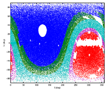
Figure 1.— Sky coverage of 5 GHz surveys in equatorial coordinates: GB6 (Gregory et al., 1996) (blue), PMNE (Griffith et al., 1995) (dark green), PMNS (Wright et al., 1994) (red), PMNT (Griffith et al., 1994) (light blue) and PMNZ (Wright et al., 1996) (magenta). The white regions are ‘holes’ in these surveys, that have been covered exploiting the NVSS and the SUMSS.

As extensively discussed by many authors in the recent past (Toffolatti et al., 1999; De Zotti et al., 1999; Mason et al., 2003; Bennett et al., 2003; Henkel & Partridge, 2005), “flat–spectrum” AGNs and QSOs, i.e. sources showing a spectral index $\alpha\simeq 0$ ($S(\nu)\propto\nu^{-\alpha}$), are expected to be the dominant source population in the range 30–100 GHz, whereas other classes of sources, and in particular the steep-spectrum sources increasingly dominating with decreasing frequency, are only giving minor contributions to the number counts at WMAP frequencies and sensitivities (De Zotti et al., 2006). We therefore chose to adopt 5 GHz as our reference frequency, and used lower frequency surveys to fill the “holes” at 5 GHz.

Altogether, the catalogues listed in Table 1 contain over 2 million sources, but we already know, from the analysis of the WMAP team, that for only a tiny fraction ($\sim 2\times 10^{-4}$) of them the WMAP data can provide useful information. Applying the MHW2 at the positions of all these sources would not only be extremely inefficient, but plainly unpractical because of the huge CPU time and disk storage requirements. Therefore, we decided to work with a complete sub-sample containing sources with $S_{5\rm GHz}\geq 500\,$mJy. This limiting flux corresponds to about 2–3 times the mean noise in the filtered images we will be dealing with (see § 3). To fill the 5 GHz “holes” we have picked up NVSS or SUMSS (in the region not covered by the NVSS) sources brighter than 500 mJy at the survey frequency. In this way we obtained an all-sky sub-sample of 4050 objects, whose spatial distribution, in Galactic coordinates, is shown in Fig. 2. After having removed sources in the strip $|b|\leq 5^{\circ}$, and in the LMC region (i.e. inside the circle of $5.5^{\circ}$ radius centered at $\alpha=5^{h}23^{m}34^{s}.7$, $\delta=-69^{\circ}45^{\prime}22^{\prime\prime}$, J2000; $l=280.47^{\circ}$, $b=-32.89^{\circ}$) and the Galactic sources outside of these zones (Taurus A, Orion A & B, and the planetary nebula IC 418/PMNJ0527-1241) we are left with 2491 objects making up our “Input Catalogue” (IC).

A cross-correlation of the IC with the WMAP catalogue (Hinshaw et al., 2006) with a search radius of $20.8^{\prime}$, equal to the dispersion of the Gaussian approximation of the beam of the lowest resolution WMAP channel ($23$ GHz), showed that $298$ of the $323$ WMAP sources have a counterpart in the IC. The other 25 WMAP sources (called missed sources) must be unusually weak at low frequency, either because have an inverted spectrum or are strongly variable and were caught in a bright phase by WMAP. They are thus interesting targets for further study, and we have investigated them too. As they have a different selection, these sources are listed separately from the others (Table 4).

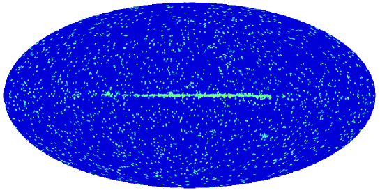
Figure 2.— Sky distribution, in Galactic coordinates, of the 4050 objects with flux densities above our selection threshold.

3. Methodology

The strategy used by the WMAP team to obtain the catalogue of 323 point sources (Hinshaw et al., 2006), summarized in § 1, used some approximations:

• The candidate detections were selected as $5\sigma$ peaks, where $\sigma$ is the rms noise defined globally. However, the removal of the Galactic emissions by component separation methods is not perfect, and leaves non-uniform contributions to the noise. Clearly, the detection, identification and flux estimation of EPS can benefit from a local treatment of the background. Furthermore, considering a global rms noise can lead to an underestimate of the error in regions of strong Galactic emission.

• The intensity peaks were fitted to a Gaussian profile. However, if the real beam response function is non-Gaussian, a Gaussian fit can lead to systematic errors in the flux estimate.

• Confusion due to other point sources that are close to the target one, albeit a less relevant effect, is another source of error that makes necessary to study the data locally.

As mentioned above, we used, locally, the MHW2 that proved to be as efficient as the matched filter but easier to implement and more stable against local power spectrum fluctuations (González-Nuevo et al. 2006; López-Caniego et al. 2006). The real symmetrized radial beam profiles given by the WMAP team have been used rather than their Gaussian approximations. The error on the source flux density is calculated locally as the rms fluctuations around the source. Finally, we also corrected the flux of all the sources for the Eddington bias, adopting a Bayesian approach (see § 3.4).

3.1. From the sphere to flat patches: rotation & projection

In order to avoid CPU and memory expensive iterative filtering in harmonic space we chose to work with small flat sky patches. For every source position in the IC and for each WMAP frequency we obtained a flat patch of approximately $14.6^{\circ}\times 14.6^{\circ}$ size, by projecting the WMAP full-sky maps. The adopted pixel area is $6.87\times 6.87\,\hbox{arcmin}^{2}$ (NSIDE=512), so that the patches are made of $128\times 128$ pixels. The patch making goes as follows:

• Given the source coordinates we obtain the corresponding pixel in the HEALPix (Górski et al., 2005) scheme.

• The image is rotated in the $a_{\ell m}$ space so that the position of the point source is moved to the equatorial plane. This is done in order to minimize the distortion induced by the projection of the HEALPix non-square pixels into flat square pixels.

• The pixels in the sphere in the vicinity of the centre are projected using the flat patch approximation and reconstructed into a 2D image in the plane.

• The units of the images are converted from mK (WMAP units) to Jy/sr and finally to Jy, using the real symmetrized radial beam profiles to do the integrals over the beam area.

The rotation/projection scheme described above introduces some distortions in the projected image. There are two different effects to be considered: a) the distortion introduced by the projection (from HEALPix pixels to flat pixels in the tangent plane); b) the distortion caused by the rotation (from HEALPix pixels to $a_{\ell m}$ and then to HEALPix pixels again). We have studied these distortions by simulating 840 sources having flux densities ranging from 500 mJy to 20 Jy with the real WMAP beam profile. First they are simulated without noise and then they are added on the combined WMAP maps, placing them at different Galactic longitudes and latitudes. Applying to each of the simulated sources the same rotation/projection procedure as for real sources we have found that, as expected, the projection effects are small at the image center (near the tangent point) and grow towards the borders of the patch. Also distortion effects are small near the equator (where the HEALPix pixels are very close to squares) and grow towards the poles. This is the main reason for performing the rotation in order to always have the point source at the equator. We find that the rotation in the $a_{\ell m}$ space from the initial position of the source to the centre of the map ($l$=0, $b$=0) has a very small effect on the flux estimate (always $<2\%$), while the effect of the projection is totally negligible.

3.2. Filters

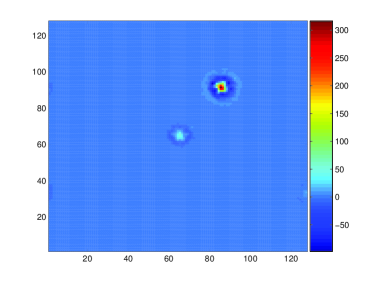
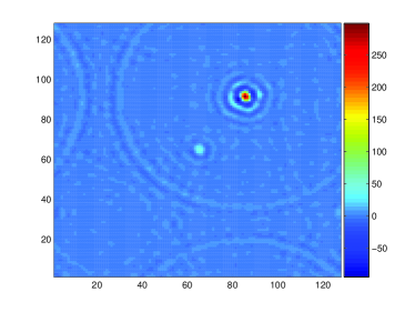
Figure 3.— Example of a bright source filtered with the MHW2 (left panel) and the MF (right panel). Strong ringing effects can be seen in the case of the MF.

In previous works (Sanz et al., 1999; Cayón et al., 2000; Sanz, Herranz, & Martínez-Gónzalez, 2001; Vielva et al., 2001a, b, 2003; Herranz et al., 2002a, b, c; González-Nuevo et al., 2006; López-Caniego et al., 2006) we have shown that application of an appropriate filter to an image helps a lot in removing large scale variations as well as most of the noise. As a result, the signal–to–noise ratio is increased, thus amplifying the point source signal. A brief summary of the fundamentals of linear filtering of two-dimensional (2D) images is given in Appendix A. In this work we have only taken into account two possible filters: the Matched Filter (MF) and the second member of the Mexican Hat Wavelet Family (MHW2). By applying these two filters to WMAP temperature maps we find that both of them give an average amplification of the EPS flux by a factor of $\sim 3$. This is a remarkable result. It means that the flux of a point source at the $\sim 2\sigma$ level in the original map can be enhanced to a $\geq 5\sigma$ level in the filtered map. In the following sub-sections, we briefly sketch the main properties of the MF and of the MHW2.

3.2.1 The Matched Filter (MF)

The MF is a circularly-symmetric filter, $\Psi(x;R,b)$, such that the filtered map, $w(R,b)$ (see Appendix A for the definition of the notation), satisfies the following two conditions: $(1)\ \langle w(R_{0},0)\rangle=s(0)\equiv A$, i.e. $w(R,0)$ is an unbiased estimator of the flux density of the source; $(2)$ the variance of $w(R,b)$ has a minimum on the scale $R_{0}$, i.e. it is an efficient estimator. In Fourier space the MF writes:

$$\psi_{MF}=\frac{1}{a}\frac{\tau(q)}{P(q)},\ \ \ a=2\pi\int dqq\frac{\tau^{2}(q)}{P(q)},$$ (2)

where $P(q)$ is the power spectrum of the background and $\tau(q)$ is Fourier transform of the source profile (equal to the beam profile for point sources). The matched filter gives directly the maximum amplification of the source and it yields the best linear estimation of the flux, when used properly and under controlled conditions. As mentioned in López-Caniego et al. (2006), the practical implementation of the MF requires the estimation of the power spectrum $P(q)$ directly from the data and this leads to a certain degradation of its performance.

The WMAP team have done a global implementation of the MF on the sphere by taking into account the non-Gaussian profile of the beam (although the source fluxes are estimated fitting the source profiles with a Gaussian). The resulting matched filter is given by eq. (1), where the flat limit quantities $\tau(q)$, $P(q)$ are replaced by their harmonic equivalents $b_{\ell}$, $C_{\ell}$. The use of the $C_{\ell}$ of the whole sky to construct a MF filter that operates in the sphere is a good first approach to obtain a list of source candidates and to estimate their fluxes, but we do believe that it can be improved by operating locally. In this paper we use different filters for regions with different levels of Galactic contamination.

3.2.2 The Mexican Hat Wavelet Family (MHWF): MHW2

One example of wavelet that is particularly well suited for point source detection is the MHW2, a member of the MHWF first introduced by González-Nuevo et al. (2006). The MHW2 is obtained by applying twice the Laplacian operator to the Gaussian function. This wavelet filter operates locally and is capable of removing simultaneously the large scale variations introduced by the Galactic foregrounds as well as the small scale structure of the noise. Note that the expression of the filter can be obtained analytically (while the MF depends on the $P(q)$ that must be estimated numerically and locally). Any member of this family can be described in Fourier space as

$$\psi_{n}(q)\propto q^{2n}e^{-q^{2}/2}.$$ (3)

The expression in real space for these wavelets is

$$\psi_{n}(x)\propto\triangle^{n}{\varphi(x)},$$ (4)

where $\varphi$ is the 2D Gaussian $\varphi(x)=(1/2\pi)e^{-x^{2}/2}$. We remark here that the first member of the family, $\psi_{1}(x)$, is the usual Mexican Hat Wavelet (MHW), that has been exploited for point source detection with excellent results (Cayón et al., 2000; Vielva et al., 2001a, 2003). Note that we call MHW$n$ the member of the MHWF with index $n$.

As already mentioned, in this work we filter our projected WMAP sky patches with the second member of the family, the MHW2. As in López-Caniego et al. (2006), we will do a qualitative comparison with the results obtained with the MF, implemented to be used locally in flat patches (at variance with the global MF used by the WMAP team).

3.3. Position, flux and error estimation

We want to obtain an estimate of the flux density, with its error, of the IC sources at the center of each filtered image. Point sources appear in the image with a profile identical to the beam profile. For example, if the beams were Gaussian, the ratio between the beam and the pixel area, $2\pi(R_{s})^{2}/L_{p}^{2}$, where $R_{s}=\mathrm{FWHM}/(2\sqrt{2\log{2}})$ is the beam width and $L_{p}$ is the pixel side, would allow us to convert the flux in the pixel where the source is located into the source flux.

In our case, the beams are not Gaussian and we will calculate this relationship integrating over the real beam profile for each channel. In carrying out the calculation we have to take into account that we work with HEALPix coordinates, at the WMAP resolution. Although the image is centered on the source position, after the projection to the flat patch the source does not always lay in the central pixel, but may end up in an adjacent one. Thus, to estimate its flux we make reference not to the intensity in the central pixel but to that of the brightest pixel close to the center of the filtered image (however in most cases the brightest pixel coincides with the central one).

At first glance, this may seem a very crude estimator, but it turns out that flux estimation through linear filtering is almost optimal in many circumstances. Let us explain how this estimator works. After filtering, the intensity of the brightest pixel can be written as a weighted sum of the intensities in the surrounding pixels,

$$w(\vec{x}_{0})=\sum_{k}\psi(\vec{x}_{k}-\vec{x}_{0})I_{p}(\vec{x}_{k})$$ (5)

where $\vec{x}_{0}$ is the position of the considered source, $I_{p}(\vec{x}_{k})$ is the intensity of the pixel of the unfiltered image located at the position $\vec{x}_{k}$ and $\psi$ is the kernel of the filter. It can be shown that if $\psi=\psi_{MF}$ (that is, for the matched filter) $w(\vec{x}_{0})$ is the best possible linear estimator (statistically unbiased and of maximum efficiency) of the flux of the source. In particular, for the case of Gaussian noise $w(\vec{x}_{0})$ is the maximum likelihood estimator of the flux of the source. As shown in López-Caniego et al. (2006) the flux estimation when $\psi=\psi_{2}$ (that is, with the MHW2) is comparable to that obtained with the MF.

The method adopted here differs from the one used by the WMAP team. They have used the MF to detect point sources above the $5\sigma$ level in the filtered images (full-sky maps, in their case), but not to estimate their fluxes. These are derived by fitting, in the unfiltered image, the pixel intensities around the point source to a Gaussian profile plus a plane baseline. However, as already noted, the profile of the source matches that of the beam, and is therefore non–Gaussian. In this paper the true source profiles are used at every step, up to the final flux unit conversions.

For each source we calculate the dispersion $\sigma$ as the square root of the variance of the background pixels that are close to the target source but are not “contaminated” by it. This number can be easily inflated in the presence of contamination by nearby sources or large scale structures that, in some cases, cannot be removed completely by filtering. In order to avoid this, we first select a shell of pixels around the source, with an inner radius equal to the FWHM of the beam. This guarantees that the source flux has decreased well below the background level. Subsequently, we choose an outer radius encompassing a sufficiently large number of pixels ($\sim 3000$) to give an accurate estimate of $\sigma$. As a final step, we divide this shell in sectors – 12, normally – and calculate their mean and dispersion. Strong contamination, due to other sources present in the annulus, shows up as a significant difference between the mean and the median; whenever this difference exceeds two times the dispersion we excluded the pixels in such sector from the calculation of the variance.

The mean values of $\sigma$, the rms error on the EPS fluxes, turn out to be: 198, 231, 222, 255 and 399 mJy at 23, 33, 41, 61 and 94 GHz, respectively. The variation of $\sigma$ with the WMAP channel is determined by the beam shapes, the spectral behavior of the foreground emission, the instrumental noise, etc.. It may be noted that these uncertainties are typically 2 or 3 times higher than the uncertainties quoted by Hinshaw et al. (2006), which are probably underestimated, as confirmed by the fact that their source counts show clear signs of incompleteness at flux densities well above $5$ times their typical errors.

3.4. Bayesian correction to the fluxes

Flux-limited surveys are affected by the well-known Eddington bias (Eddington, 1940) that leads to an overestimate of the flux of faint sources. Hogg & Turner (1998) have shown how to correct for this effect if the underlying distribution of source fluxes is known. Unfortunately, our knowledge of this distribution in the frequency range covered by WMAP is rather poor. However, as shown in the Appendix B, given a set of observed fluxes and the associated values of the rms noise it is possible to simultaneously estimate the slope of the flux distribution (i.e., of the differential number counts) and to obtain an unbiased estimate of the source fluxes. We have applied this method, based on the Bayesian approach introduced by Herranz et al. (2006), to correct for the Eddington bias. The estimated slopes of the differential number counts are 2.11, 2.34, 2.16, 2.14, and 2.16 for the 23, 33, 41, 61, and 94 GHz channels, respectively, in very good agreement with the results of the ATCA 18 GHz survey (Ricci et al. 2004: $2.2\pm 0.2$), of the 9C survey at 15 GHz (Waldram et al. 2003: $2.15$), and of the 33 GHz VSA survey (Cleary et al. 2005: $2.34^{+0.25}_{-0.26}$).

4. The New Extragalactic WMAP Point Source (NEWPS) catalogue

4.1. Comparison between MHW2 and MF

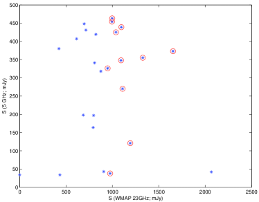
Figure 4.— 5 GHz vs 23 GHz WMAP flux densities of the 25 sources missed by our low-frequency selection. The source with zero 23 GHz flux was not detected at 23 GHz, but at least at one higher frequency. Encircled dots are sources that we recover at $\geq 5\sigma$.

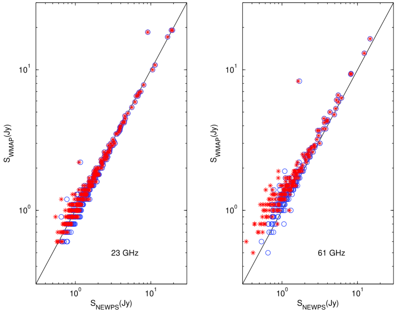
Figure 5.— Comparison of $NEWPS_{3\sigma}$ with WMAP flux densities at 23 and 61 GHz: Blue circles show our uncorrected fluxes and red asterisks the corrected ones.

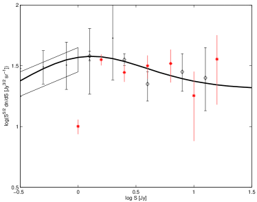
Figure 6.— Number counts multiplied by $S^{5/2}$. Red asterisks: counts from the $NEWPS_{5\sigma}$ catalogue at 33 GHz (see text for more details). Black diamonds: WMAP counts (Hinshaw et al., 2006). Black dots: ATCA 18 GHz pilot survey counts (Ricci et al., 2004). The parallelogram is from the DASI experiment at 31 GHz (Kovac et al., 2002). The solid curve shows, for comparison, the counts predicted by the model by De Zotti et al. (2005).

We have carried out the detection/flux estimation process using the two different filters, MHW2 and MF, previously discussed. We have found that filtering with the MF introduces ringing effects around the target EPS in at least 15% of the images analyzed (see Figure 3). These effects are stronger for the brightest sources. Rings appear due to strong oscillations in the shape of the matched filter which are determined by sharp features in the angular power spectrum of temperature anisotropies in the sky patch. These sharp features are likely to appear in regions showing a high background signal and/or in regions where point sources constitute a major component of the total intensity of the image. If the number of images were small, we could check the images one–by–one visually and study separately the anomalous cases, but this procedure is impractical in the present context. With a blind approach we get a number of spurious sources, mainly due to positive interferences between rings. In the case of our non-blind approach rings may also contaminate surrounding pixels, thus affecting the error estimates and the flux estimates of the surrounding sources. On the contrary, we found that the MHW2 filter does not introduce ringing effects in any of the considered images.

The number of source detections above a certain $n\sigma$ threshold obviously depends on the correct estimation of the background noise level. Ringing effects affect negatively such estimate. We find that, on average, by filtering with the MHW2 we correctly identify $\sim 7\%$ more sources than with the MF. For this reason we decided to build the final catalogue using the detections/flux estimates obtained with the MHW2.

4.2. $NEWPS_{3\sigma}$

To define our first SubCatalogue (SC), $NEWPS_{3\sigma}$, of sources at $\geq 3\sigma$ we need to take into account that the IC was generated from surveys with angular resolution $\leq 4^{\prime}.2$, i.e. much higher than the WMAP resolution, so that we may have multiple IC sources within one WMAP beam. In some cases the WMAP signal is entirely due to the brightest source within the beam, whose flux, attenuated by the response function, accounts also for the signal detected in the direction of nearby sources. The latter are therefore false detections that we have removed from the sample. A search within circles of radius equal to 2 WMAP beam sizes (beam size=FWHM$/2\sqrt{2\log(2)}$) centered on the position of each source, starting from the brightest ones, has yielded numbers of false detections decreasing from 354 at 23 GHz to 104 at 94 GHz.

The contamination of very bright sources can actually extend beyond 2 WMAP beam sizes. We have therefore repeated the above search up to 4 beam sizes, and removed those sources for which the contamination by the bright source accounts for more than 50% of the detected signal. The number of such cases oscillate around 7 at all channels. In 13% of the cases, the data are consistent with more than one IC source contributing significantly to the WMAP flux.

After having removed the 4 $|b|>5^{\circ}$ sources known to be Galactic (Taurus A, Orion A & B, and IC 418), we are left with 760(738+22 missed sources, WMAP sources that are not included in our IC), 565(547+18), 536(518+18), 366(360+5) and 103(101+2) EPS with signal-to-noise ratios $>3$ in the 23, 33, 41, 61, and 94 GHz channels, respectively (see Table 2). Finally, a cross correlation of the catalogues at the different frequencies shows that we have 933 (908+25) different EPS with signal-to-noise ratios $>3$ in at least one WMAP channel, which constitutes our $NEWPS_{3\sigma}$ Catalogue.

4.3. $NEWPS_{5\sigma}$: A robust subsample

Of the 381 sources that we detected at $\geq 5\sigma$ ($NEWPS_{5\sigma}$ Catalogue in Table 4, see Appendix C., plus 12 EPS detected at $>5\sigma$ listed in Table 5) only 283 are listed in the WMAP 3-yr catalogue (see Table 3 for a better understanding of the detection statistics). As expected, the a priori knowledge of source positions has allowed us to significantly increase the detection efficiency. Additionally, in our approach, 39 (26+13) WMAP sources present a signal-to-noise ratio $<5$ (as shown in Table 3) .

Regarding the reliability of the detected sources near the $5\sigma$ threshold, we would expect that most of them, if not all, are actually real $5\sigma$ sources. Since we have followed a non-blind approach we know that there is a real source in every position we have considered, but it is possible that a very weak source appears above this threshold because it has been contaminated, e.g. by Galactic foregrounds, CMB, etc. In order to check this possibility we have created a catalogue of false positions and we have repeated the process of rotation, projection, filtering of each patch and flux estimation exactly in the same way as we have done for detecting the sources in $NEWPS_{5\sigma}$. Then we have counted the number of $>5\sigma$ detections. This number gives an idea of how likely is that the foregrounds produce a spurious $>5\sigma$ detection and therefore how reliable is our catalog for that threshold.

This catalogue of false positions is obtained by shifting 10 degrees in the longitude coordinate the position in the sky of each source outside $|b|>5^{\circ}$ in the IC. We have performed this test only at 23 GHz, because at this frequency we have the highest number of detections and the lowest mean value of rms noise. As a result, we have found $3\%$ of spurious $>5\sigma$ detections in the analysed patches, which is in agreement with the numbers discussed by Bennett et al. (2003) and Hinshaw et al. (2006).

In addition, as already mentioned, there are 25 WMAP sources left out by our low-frequency selection, but included in our analysis (see Table 4). Only 12 of them are detected at $\geq 5\sigma$ by our approach, and only 3 have 23 GHz flux densities above the estimated completeness limit of 1.1 Jy (see Fig. 6). Of our 12 sources which are $\geq 5\sigma$ detections, 10 have low-frequency flux densities $\geq 270\,$mJy (8 of them are above 340 mJy) and may well be variable sources, that happened to be in a particularly ‘high’ phase at the time of WMAP observations. The source with $S_{5{\rm GHz}}=120\,$mJy has an inverted spectrum (i.e. a spectrum rising with frequency) and the last one, with $S_{5{\rm GHz}}=38\,$mJy, is a strong candidate to be a spurious source.

Finally, by exploiting the distribution of spectral indexes $\alpha_{5}^{23}$, we could also tentatively estimate how many more $5\sigma$ detections we missed at 23 GHz because of the adopted 5 GHz flux limit $S_{5GHz}\geq 500$ mJy. From the observationally determined number counts at 5 GHz (and the associated uncertainties) we estimate that there should be $\sim$2100-2500 sources in the flux range $300<S_{5GHz}<500$ mJy, in the same sky area in which we find 2491 sources with $S\geq 500$ mJy. For being detectable at 23 GHz, these sources should show an inverted spectrum with slope $\alpha\leq-0.63$. The distribution of the spectral indexes $\alpha_{5}^{23}$ of sources in the IC shows that only $\leq 1$% of them show spectra so inverted. This implies that we may expect $\leq 20$–25 sources with $300<S_{5GHz}<500$ to be detectable at $\geq 5\sigma$ at 23 GHz. The number of expected detections decreases to $\leq 5$ for $100<S_{5GHz}<300$, and is essentially zero at still fainter 5 GHz fluxes. These estimates are comparable with the number (11) of sources at 23 GHz (see Table 3) detected by WMAP but missed by our selection criterion. Note that, at higher frequencies, the numbers of missed detections, which is more difficult to estimate due to the higher errors in flux, decreases in parallel with the decrease of the number of detections (see Table 2 and Section 5.1).

5. Results and discussion

Table 1Summary of the large-area surveys of point sources used in this work.

Frequency	Catalogue	$S_{lim}$(mJy)	DEC range			Angular resolution
	GB6	18	0	—	+75	3.5’	Gregory et al. (1996)
	PMNE	40	-9.5	—	+10	4.2’	Griffith et al. (1995)
4.85 GHz	PMNT	42	-29	—	-9.5	4.2’	Griffith et al. (1994)
	PMNZ	72	-37	—	-29	4.2’	Wright et al. (1996)
	PMNS	20	-87.5	—	-37	4.2’	Wright et al. (1994)
1.4 GHz	NVSS	2.5	-40	—	+90	45”	Condon et al. (1998)
0.843 GHz	SUMSS	18	-50	—	-30	45”$\hbox{cosec}|\delta|$	Mauch et al. (2003)
		8	-90	—	-50	45”$\hbox{cosec}|\delta|$

Table 2Summary of the results.

	23 GHz	33 GHz	41 GHz	61 GHz	94 GHz	Total
$\textless$ rms $\textgreater$	198	231	222	255	399	–
$\alpha$	2.11	2.34	2.16	2.14	2.16	–
$NEWPS_{3\sigma}$	760	565	536	366	103	933
	(738+22)	(547+18)	(518+18)	(360+6)	(101+2)	(907+25)
$NEWPS_{5\sigma}$	350	224	218	136	22	381
	(339+11)	(219+5)	(215+3)	(135+1)	(22+0)	(369+12)
WMAP 5$\sigma$	314	292	280	154	29	323

Note. — The “rms” of the patches is in units of mJy. The slope $\alpha$ corresponds to the estimated slope of the flux distribution (i.e. of the differential number counts, dN/dS $\propto S^{-\alpha}$ ). For the $NEWPS_{5\sigma}$ and $NEWPS_{3\sigma}$ we show in parenthesis the number of detections coming from the initial catalogue “IC” and the number of detections among the 25 WMAP objects not present in IC (missed sources, see Table 4).

Table 3Detection statistics

	(All $\nu$)	(All $\nu$)	(23 GHz)	(23 GHz)
SubCatalogue (SC):	$3\sigma$	$5\sigma$	$5\sigma$	$\geq$ $S_{lim}$ 1.1Jy
Number of WMAP EPS $\in$ SC	297	271	258	186
Number of WMAP EPS $\notin$ SC	—	26	39	111
Number of Missed EPS $\in$ SC	25	12	11	3
Number of Missed EPS $\notin$ SC	—	13	14	22
Dropped WMAP EPS	1	1	1	1
New EPS ($\notin$ in WMAP)	611	98	81	43

Note. — Distribution of the detected sources in different subsamples. The description has been made for 4 classes of EPS: WMAP EPS (WMAP sources that appeared in our IC), Missed EPS (WMAP EPS NOT included in our IC), Dropped EPS (the planetary nebula IC418 (PMNJ0527-1241)) and New EPS (detected EPS NOT included in the WMAP EPS catalogue). The total number of sources in each subCatalogue, detected by the MHW2 filter, are given by the sum of the entries in lines (1)+(3)+(6), in agreement with the numbers in Table 2.

5.1. $NEWPS_{5\sigma}$ versus WMAP sources

The WMAP 3-year catalogue (Hinshaw et al. 2006) lists 314, 292, 280, 154, and 29 $\geq 5\sigma$ detections at 23, 33, 41, 61, and 94 GHz, respectively, to be compared with 350 (339+11 missed sources), 224 (219+5), 218 (215+3), 136 (135+1) and 22 sources in the $NEWPS_{5\sigma}$ catalogue (see Table 2). Although the blind WMAP technique yielded a lower number of detections at 23 GHz and a lower total number, it was apparently more successful in retrieving sources at $\geq 5\sigma$ in different channels. This may be, to some extent, related to their lower error estimates. However, note that the same sources can be detected in different channels. Therefore, the total number is the intersection of the channels, giving a global a reduced number for the WMAP case (323 vs. 381).

In Fig. 5 we compare our flux estimates for sources in the $NEWPS_{3\sigma}$ catalogue with the WMAP ones at 2 frequencies (23 and 61 GHz). We have plotted the corrected fluxes (red asterisks) as well as the uncorrected ones (blue circles) to show the effect of the Bayesian correction. At 23 GHz the agreement is generally good and the correction makes no difference for fluxes $\gtrsim 1.5\,$Jy, due to the fact that almost all the sources are detected at high signal to noise ratios.

The most striking difference is found for Fornax A (catalog ) (PMNJ0321-3658), represented by the isolated point on the top right-hand corner of the 23 GHz channel and at the center of the upper part of the 61 GHz panel. Our procedure yields 23 GHz and 61 GHz flux densities of $9.1\pm 0.2$ and $1.6\pm 0.2$ Jy, to be compared with $18.5\pm 3.6$ and $8.3\pm 2.1$ Jy, respectively, given in the WMAP catalogue (fluxes obtained by aperture photometry). The problem here is that Fornax A has a relatively weak core and 2 big lobes extending, altogether, over $\simeq 1^{\circ}$, so that it cannot be treated as a point source, even at the relatively low resolution of WMAP. As both flux estimates are not reliable we have applied the NRAO Astronomical Image Processing System (AIPS) software to the unfiltered patches, fitting the source to a gaussian. The values obtained by this method are $11.49\pm 0.63$ and $0.92\pm 0.72$ Jy, with a best fit major(minor) axis of $1.18^{\circ}(0.81^{\circ})$. Resolution effects may be worrisome also for Centaurus A (catalog ) (PMNJ1325-4257), the largest radio source in the sky at low frequencies, which is however not present in the WMAP catalog. Therefore for this source too we have checked our flux estimates with those obtained from AIPS, which gave $48.12\pm 0.04$ and $20.31\pm 0.72$ Jy, for 23 GHz and 61 GHz respectively, and a best fit major (minor) axis of $1.13^{\circ}(0.84^{\circ})$ for 23 GHz, in good agreement with our results.

The second discrepant point (circle not far from the panel center at 23 GHz) is PMN J0428-3756 (catalog ) for which we get a 23 GHz flux of 1.12 Jy, while the WMAP flux is 2.20 Jy. This source is an ATCA flux calibrator. Its light curve at 20 GHz shows its flux increasing from $\simeq 1\,$Jy in 2002 to a maximum of 2.04 Jy in 2004, and steadily decreasing afterwards back to $\simeq 1\,$Jy in 2006.

The asterisks in the lower left-hand part of each panel correspond to objects that we detect at $<5\sigma$ at 23 GHz, whose flux density is substantially decreased by the correction for the Eddington bias.

At 61 GHz WMAP flux densities are systematically brighter than ours by $\simeq 10\%$. This may be due to the use by the WMAP team of Gaussian source profiles while, as discussed by Hinshaw et al. (2006), beams increasingly deviate from Gaussianity with increasing frequency. On the other hand, we have taken into account real symmetrized beam profiles. At this frequency many sources fainter than $\simeq 2\,$Jy are detected by our procedure at $<5\sigma$ and have substantial corrections for the Eddington bias, moving them to the left of the diagram.

5.2. Source number counts

In Figure 6 we compare the number counts derived from the $NEWPS_{5\sigma}$ catalogue at 33 GHz (red asterisks with Poisson error bars) with other sets of observational data, specified in the caption, and with the prediction of the model by De Zotti et al. (2005). The agreement is clearly good. The completeness flux limit of our catalogue is around $\sim$1.1 Jy, as expected from the average value of the flux error at this frequency, $\simeq 230\,$mJy.

Hinshaw et al. (2006) estimated the contribution of point sources below the detection threshold to the anisotropy power spectrum at 40.7 GHz to be $A=0.017\pm 0.002\,\mu\hbox{K}^{2}$. Again, this is in good agreement with the De Zotti et al. (2005) model, yielding, at this frequency, $A=0.018\,\mu\hbox{K}^{2}$.

6. Conclusions

We have used the MHW2 filter (González-Nuevo et al. 2006) to obtain estimates of (or upper limits on) the flux densities at the WMAP frequencies of a complete all-sky sample of 2491 sources at $|b|>5^{\circ}$, brighter than 500 mJy at 5 GHz (or at 1.4 or 0.84 GHz, in regions not covered by 5 GHz surveys but covered by either the NVSS or the SUMSS). We have shown that the MHW2 filter has an efficiency very similar to the MF and is much easier to use.

We have obtained flux density estimates for the 933 sources detected at $\geq 3\sigma$, our $NEWPS_{3\sigma}$ Catalogue (see Section 4.2). Of the 381, presumably extragalactic, sources detected at $\geq 5\sigma$, 369 of which constitute our $NEWPS_{5\sigma}$ Catalogue (Section 4.3), 98 (i.e. 26%) are “new”, in the sense that they are not present in the WMAP catalogue; 43 of them are above the estimated completeness limit of the WMAP survey: $\simeq 1.1$ Jy at 23 GHz. This illustrates how the prior knowledge of source positions can help their flux measurements.

On the other hand, 39 (23+13) WMAP extragalactic sources with low-frequency counterparts included in our sample were detected by us at $<5\sigma$. This is probably due to the fact that our error estimates exceed substantially those given by the WMAP team, particularly at 23 GHz, where we have the highest detection rate. In fact, the WMAP errors do not correspond to the rms fluctuations in the source neighborhood but to the uncertainties in the amplitude of the Gaussian fit. As a consequence, the WMAP catalogue starts being incomplete at flux densities more than 2 times higher than 5 times their typical formal errors.

Our flux density estimates for sources detected at $\geq 5\sigma$ are generally in very good agreement with the WMAP ones at 23 GHz. At higher frequencies WMAP fluxes tend to be slightly but systematically higher than ours, probably due to having ignored the deviations, increasing with frequency, of the point spread function from a Gaussian shape. Our estimates use the real beam shape at every frequency. For only one source we have a strong discrepancy with WMAP. Such source, Fornax A, is known to have powerful lobes extending over $\sim 1^{\circ}$, and is therefore resolved by WMAP. Thus, the point source assumption on which both WMAP and our flux estimates rely, is clearly not appropriate and yields unreliable results. A smaller, but still significant, discrepancy, is found for PMN J0428-3756.

We have also worked out and applied a method to correct flux estimates for the Eddington bias, without the need of an a-priori knowledge of the slope of source counts below the detection limit.

Our selection criterion leaves out 25 WMAP sources, only 12 of which however turn out to be $\geq 5\sigma$ detections after our analysis, and only 3 have 23 GHz fluxes $\gtrsim 1.1\,$Jy, the estimated completeness limit of the survey. Thus, our approach has proven to be competitive with, and complementary to the blind technique adopted by the WMAP team. In fact we missed 3 sources brighter than the estimated completeness limit ($S_{23\rm GHz}=1.1\,$Jy), but we detected 42 new ones.

On the whole, 26% of sources we have detected at $\geq 5\sigma$ are not present in the WMAP catalogue. On the other hand, the efficiency of the process is low. Only 381 of the 2491 sources in our input sample were detected at $\geq 5\sigma$ in at least one WMAP channel.

In a forthcoming paper, we will exploit our catalogue to investigate the high-frequency properties of sources selected at low frequencies.

Appendix A Linear filters in two dimensions

The approach adopted in this paper assumes that in the center of each image (sky patch) there is a point source with unknown flux density, $A$. As usual we describe the source as

$$s(\vec{x})=A\tau(\vec{x}),$$ (A1)

where $\tau(\vec{x})$ is the source profile. We will assume circular symmetry, so that $\tau(\vec{x})=\tau(x)$, $x=|\vec{x}|$. For point sources the profile is equal to the beam response function of the detector. For a circular Gaussian beam we have

$$\tau(x)=e^{-x^{2}/2R_{s}^{2}},$$ (A2)

where $R_{s}$ is the angular radius of the beam response function. In the Fourier space the beam profile of eq. (A2) is

$$\tau(q)=e^{-q^{2}R_{s}^{2}/2},$$ (A3)

where $q\equiv|\vec{q}|$. Actually the WMAP beams are not Gaussian and we will use the real symmetrized radial beam profiles for the different WMAP channels to construct our filters.

Let us consider a 2D–filter $\Psi(\vec{x};R,\vec{b})$, where $R$ and $\vec{b}$ define a scaling and a translation respectively. Then

$$\Psi(\vec{x};R,\vec{b})\equiv\frac{1}{R^{2}}\psi\left(\frac{|\vec{x}-\vec{b}|}{R}\right).$$ (A4)

If we filter our field $f(\vec{x})$ with $\Psi(\vec{x};R,\vec{b})$, the filtered map will be

$$w(R,\vec{b})=\int d\vec{x}\,f(\vec{x})\Psi(\vec{x};R,\vec{b}).$$ (A5)

The filter normalization preserves the amplitude of the source at its position ($b=0$) after filtering:

$$\int d\vec{x}\,\tau(\vec{x})\Psi(\vec{x};R,\vec{0})=1.$$ (A6)

The n-th moment of the filtered map is defined as

$$\sigma_{n}^{2}\equiv 2\pi\int_{0}^{\infty}dq\ q^{1+2n}P(q)\psi^{2}(q).$$ (A7)

where $P(q)$ is the power spectrum of the unfiltered map and $\psi(q)$ is the Fourier transform of $\psi(x)$:

$$\psi(q)=\int_{0}^{\infty}dx\,xJ_{0}(qx)\psi(x).$$ (A8)

Here $\vec{q}$ is the wave number, $q\equiv|\vec{q}|$ and $J_{0}$ is the Bessel function of the first kind. The zeroth-order moment, $\sigma_{0}$, which is the dispersion of the filtered map, will be denoted, for simplicity, as $\sigma$. It is a function of the filter scaling $R$, of the source profile $\tau$ and of the power spectrum $P(q)$ of the unfiltered image. Then, for a given image and a given source profile it is possible to optimize the ratio $A/\sigma$ just by modifying the scaling $R$. The scale $R_{0}$ at which $A/\sigma$ is maximum is called optimal scale. It has been shown (Vielva et al., 2001a, 2003; López-Caniego et al., 2004, 2005) that, working at this scale at which a filter maximizes the flux of a compact source with respect to the average surrounding background, the filter performance in detecting point sources and estimating their flux is maximized.

Appendix B Derivation of the Bayesian correction formulae

B.1. The Eddington bias

The distribution, normalized to unity, of true fluxes, $S$, of extragalactic sources, is usually well described by a power law

$$P(S|q)=kS^{-(1+q)},\ \ \ S\geq S_{m}$$ (B1)

where the normalization $k$ is

$$k=q{S_{m}}^{q},\ \ \ q>0.$$ (B2)

The observed fluxes are contaminated by noise. Let $\mathbf{S^{o}}=\{S^{o}_{1},\ldots,S^{o}_{N}\}$ be the observed fluxed of the $N$ galaxies detected above a given flux threshold and $\mathbf{S}=\{S_{1},\ldots,S_{N}\}$ their true fluxes. In the case of Gaussian noise we have

$$P\left(\mathbf{S^{o}}\big{|}\mathbf{S},q\right)\propto\mathrm{exp}\left[-\frac{1}{2}\sum_{i=1}^{N}\left(\frac{S^{o}_{i}-S_{i}}{\sigma_{i}^{2}}\right)^{2}\right]\ ,$$ (B3)

where $\sigma_{i}$ is the rms noise for the $i$th source. Since we select only sources above a certain threshold, a selection effect appears: sources whose intrinsic flux is lower than the detection threshold may be detected due to positive noise fluctuations and, on the other hand, sources that should be detected because their flux is greater than the detection threshold may be missed due to negative fluctuations. Since according to eq. (B1) there are more faint than bright sources we end up with an excess of sources whose flux is overestimated. This is the Eddington bias (Eddington, 1940).

B.2. Bayesian slope determination and flux correction

¿From the Bayes’ theorem we have

$$P\left(\mathbf{S},q\big{|}\mathbf{S^{o}}\right) = \frac{P\left(\mathbf{S^{o}}\big{|}\mathbf{S},q\right)P(\mathbf{S},q)}{P(\mathbf{S^{o}})}$$ (B4)

$$\propto P\left(\mathbf{S^{o}}\big{|}\mathbf{S},q\right)P(\mathbf{S}|q)P(q).$$

We will assume that $P(q)$ is uniform, that the source fluxes take values drawn at random from the distribution of eq. (B1), and that the flux of any given source is independent of the fluxes of the other sources. Therefore

$$P\left(\mathbf{S}\big{|}q\right)=\prod_{i=1}^{N}P(S_{i}|q)=q^{N}S_{m}^{Nq}\left(\prod_{i=1}^{N}S_{i}\right)^{-(q+1)}.$$ (B5)

Therefore, using eqs. (B3) and (B4) we have

$$P\left(\mathbf{S},q\big{|}\mathbf{S^{o}}\right) \propto \mathrm{exp}\left[-\frac{1}{2}\sum_{i=1}^{N}\left(\frac{S^{o}_{i}-S_{i}}{\sigma_{i}^{2}}\right)^{2}\right]\times$$ (B6)

$$q^{N}S_{m}^{Nq}\left(\prod_{i=1}^{N}S_{i}\right)^{-(q+1)}.$$

If the slope $q$ is known, the maximum likelihood estimator of the fluxes of the sources is easily calculated (Hogg & Turner 1998):

$$S_{i}=\frac{S^{o}_{i}}{2}\left[1+\sqrt{1-\frac{4(1+q)}{r_{i}^{2}}}\right],\ \ \ r_{i}\geq 2\sqrt{1+q},$$ (B7)

where $r_{i}=S^{o}_{i}/\sigma_{i}$ is the signal to noise ratio of the source. Conversely, if the true intrinsic fluxes of the sources $\mathbf{S}$ were known and the slope $q$ unknown, the maximum likelihood estimator for the value of $q$ would be

$$q=\left[\frac{1}{N}\sum_{i=1}^{N}\mathrm{ln}\left(\frac{S_{i}}{S_{m}}\right)\right]^{-1}.$$ (B8)

Unfortunately, in many cases, and particular in the case of WMAP surveys, neither $q$ nor $\mathbf{S}$ are known a priori. Then it is necessary to solve simultaneously for the two unknowns. A way to do this is to introduce eq. (B7) into eq. (B8), which gives the implicit equation

$$\frac{1}{q}=\frac{1}{N}\sum_{i=1}^{N}\left[\mathrm{ln}\left(\frac{S^{o}_{i}}{S^{o}_{m}}\right)+\mathrm{ln}\left(\frac{1+\Delta_{i}}{1+\Delta_{m}}\right)\right],$$ (B9)

where

$$\Delta_{i}=\sqrt{1-\frac{4(1+q)}{r_{i}^{2}}}.$$ (B10)

Equation (B9) can be solved numerically if the minimum signal to noise ratio of the galaxies considered satisfies the condition $r_{m}^{2}\geq 4(1+q)$. Once $q$ is estimated, the fluxes $\mathbf{S}$ can be estimated using eq. (B7).

The asymptotic limits of the estimators, valid in the high signal to noise regime, that is, for $r_{m}\gg q$, are:

$$q \simeq \left[\frac{1}{N}\sum_{i=1}^{N}\mathrm{ln}\left(\frac{S^{o}_{i}}{S^{o}_{m}}\right)\right]^{-1}$$ (B11)

$$S_{i} \simeq S^{o}_{i}\left[1-\frac{1+q}{r_{i}^{2}}\right].$$ (B12)

Appendix C $NEWPS_{5\sigma}$ source catalogue

The $NEWPS_{5\sigma}$ Catalogue consists of 369 entries corresponding to all the EPS detected in the WMAP 3-yr full-sky maps at the $>5\sigma$ level, after filtering with the MHW2 as discussed in the text. The 25 missed sources (WMAP detected sources that did not appear in our IC) are listed in Table 4 while the 369 IC sources detected at $>5\sigma$ are presented in Table 5. For each EPS in the Catalogue, and from left to right, we list the following data: the Equatorial, $\alpha$, $\delta$, coordinates of the center of the pixel; the NON CORRECTED source fluxes, $S_{\nu}$, in each WMAP channel identified by the channel symbols (K, Ka, Q, V and W) and their corresponding estimated errors ($\sigma$), in Jy; the position in the 3-year WMAP catalogue; the closest source present in the PMN or GB6 catalogues or the brightest NVSS or SUMSS source within the resolution element (i.e., inside the FWHM of the beam of the given WMAP frequency channel) and a “M” label that means that at least another source inside the beam has a 5 GHz flux within a factor of 2 from the brightest one, that we list as the likely identification. Table 4 has an additional column listing the 5 GHz fluxes. For those sources not detected at $\geq 5\sigma$, we have used “–” in the corresponding channel column.

Table 4Missed EPS

RA	Dec	K($\sigma$)	Ka($\sigma$)	Q($\sigma$)	V($\sigma$)	W($\sigma$)	S5GHz	WMAP	low freq. id.
h	deg	Jy(Jy)	Jy(Jy)	Jy(Jy)	Jy(Jy)	Jy(Jy)	Jy
0.434	-35.197	1.19 (0.15)	0.96 (0.21)	1.25 (0.20)	1.06 (0.26)	0.82 (0.38)	0.12	6	PMNJ0026-3512
0.493	5.922	1.09 (0.16)	1.43 (0.22)	0.89 (0.21)	0.74 (0.26)	1.22 (0.45)	0.35	7	PMNJ0029+0554
5.229	-20.268	0.71 (0.17)	0.51 (0.20)	0.50 (0.21)	0.41 (0.23)	0.25 (0.38)	0.43	68	PMNJ0514-2029
5.321	-5.675	2.07 (0.63)	1.43 (0.82)	1.06 (0.67)	0.41 (0.45)	0.15 (0.56)	0.04	71	PMNJ0520-0537
5.427	-48.449	1.04 (0.16)	1.25 (0.24)	1.25 (0.28)	0.63 (0.25)	1.03 (0.40)	0.42	74	PMNJ0526-4830
5.680	-54.277	1.65 (0.17)	1.52 (0.20)	1.79 (0.18)	1.22 (0.21)	0.50 (0.31)	0.37	77	PMNJ0540-5418
5.839	-57.551	1.33 (0.18)	0.94 (0.21)	1.14 (0.19)	0.54 (0.21)	0.59 (0.34)	0.35	79	PMNJ0550-5732
6.003	-45.466	0.61 (0.20)	0.95 (0.21)	0.60 (0.20)	0.66 (0.23)	0.21 (0.39)	0.41	81	PMNJ0559-4529
8.273	-24.423	1.11 (0.18)	0.73 (0.21)	0.87 (0.21)	0.64 (0.25)	0.32 (0.40)	0.27	108	PMNJ0816-2421
10.544	41.306	1.10 (0.18)	1.02 (0.20)	0.92 (0.21)	0.87 (0.26)	0.94 (0.42)	0.44	133	GB6 J1033+4115
11.034	-44.011	0.70 (0.19)	0.92 (0.21)	0.77 (0.20)	0.35 (0.22)	0.23 (0.34)	0.45	142	PMNJ1102-4404
11.829	-79.554	0.97 (0.18)	0.69 (0.28)	0.51 (0.24)	0.41 (0.23)	0.10 (0.41)	0.04	152	PMNJ1150-7918
12.056	48.104	0.79 (0.24)	0.67 (0.22)	0.67 (0.23)	0.62 (0.22)	0.14 (0.34)	0.16	156	GB6 J1203+4803
12.464	11.406	0.00 (0.00)	0.86 (0.32)	0.88 (0.24)	0.53 (0.27)	0.43 (0.56)	0.03	162	GB6 J1228+1124
12.519	13.857	0.91 (0.29)	0.49 (0.35)	0.39 (0.25)	0.76 (0.30)	0.20 (0.54)	0.04	165	GB6 J1231+1344
13.047	48.947	0.43 (0.18)	0.64 (0.21)	0.68 (0.18)	0.61 (0.21)	1.09 (0.31)	0.03	170	GB6 J1303+4848
13.559	27.396	0.88 (0.21)	0.81 (0.26)	0.68 (0.27)	0.52 (0.25)	1.46 (0.35)	0.32	181	GB6 J1333+2725
14.668	49.973	0.69 (0.18)	1.01 (0.22)	0.84 (0.20)	0.45 (0.25)	0.74 (0.33)	0.20	196	GB6 J1439+4958
16.807	41.239	0.80 (0.22)	0.71 (0.31)	0.71 (0.27)	0.29 (0.23)	0.00 (0.38)	0.20	222	GB6 J1648+4104
16.994	68.495	0.42 (0.17)	0.64 (0.18)	0.72 (0.16)	0.79 (0.19)	0.52 (0.29)	0.38	228	GB6 J1700+6830
17.128	1.786	1.00 (0.20)	0.93 (0.24)	0.80 (0.19)	0.76 (0.28)	0.70 (0.45)	0.46	230	PMNJ1707+0148
17.618	-79.578	0.82 (0.18)	0.78 (0.20)	0.81 (0.18)	0.74 (0.21)	0.69 (0.38)	0.42	235	PMNJ1733-7935
22.496	-20.853	0.95 (0.13)	0.83 (0.20)	0.78 (0.23)	0.70 (0.27)	1.28 (0.47)	0.33	297	PMNJ2229-2049
22.939	-20.191	1.00 (0.20)	0.61 (0.22)	0.76 (0.24)	0.80 (0.30)	0.41 (0.45)	0.45	305	PMNJ2256-2011
23.266	-50.286	0.81 (0.18)	1.12 (0.18)	0.77 (0.19)	0.80 (0.23)	0.61 (0.35)	0.34	307	PMNJ2315-5018

Table 5$NEWPS_{5\sigma}$ source catalogue

RA	Dec	K($\sigma$)	Ka($\sigma$)	Q($\sigma$)	V($\sigma$)	W($\sigma$)	WMAP	low freq. id.
h	deg	Jy(Jy)	Jy(Jy)	Jy(Jy)	Jy(Jy)	Jy(Jy)
0.103	-6.481	2.7 (0.2)	2.3 (0.2)	2.4 (0.2)	2.2 (0.3)	–	1	PMNJ0006-0623
0.214	-39.957	1.3 (0.2)	1.2 (0.2)	–	–	–	2	PMNJ0013-3954
0.326	26.031	1.1 (0.2)	–	–	–	–	3	NVSS J001939+260245	M
0.328	20.445	1.0 (0.2)	–	–	–	–	4	GB6 J0019+2021
0.424	-26.067	1.1 (0.2)	–	–	–	–	5	PMNJ0025-2602	M
0.789	-25.251	1.2 (0.2)	–	–	–	–	9	PMNJ0047-2517
0.790	-73.125	1.9 (0.2)	1.4 (0.2)	1.5 (0.2)	–	–		PMNJ0047-7308
0.827	-57.637	1.4 (0.2)	1.2 (0.2)	0.9 (0.2)	–	–	10	PMNJ0050-5738
0.847	-9.429	1.1 (0.2)	–	–	–	–	13	PMNJ0050-0928
0.854	-6.828	1.2 (0.2)	–	–	–	–	11	PMNJ0051-0650
0.962	30.412	–	1.2 (0.2)	–	–	–		GB6 J0057+3021
0.987	-72.215	2.3 (0.2)	1.4 (0.2)	1.4 (0.2)	–	–		PMNJ0059-7210
1.099	48.322	–	1.2 (0.2)	–	–	–		GB6 J0105+4819
1.115	-40.584	1.8 (0.1)	1.9 (0.2)	1.7 (0.2)	1.1 (0.2)	–	14	PMNJ0106-4034
1.140	1.583	2.6 (0.2)	2.3 (0.3)	2.2 (0.2)	2.0 (0.3)	–	16	PMNJ0108+0134
1.152	13.335	1.4 (0.2)	1.1 (0.2)	–	–	–	15	GB6 J0108+1319
1.270	-11.686	1.4 (0.2)	1.1 (0.2)	1.3 (0.2)	1.4 (0.3)	–	18	PMNJ0116-1136
1.318	-21.685	0.8 (0.2)	–	–	–	–		PMNJ0118-2141
1.361	11.807	1.2 (0.2)	–	1.1 (0.2)	–	–	19	GB6 J0121+1149
1.379	25.070	1.0 (0.2)	–	–	–	–		GB6 J0122+2502
1.421	-0.082	1.2 (0.2)	–	–	–	–	20	PMNJ0125-0005
1.544	-16.863	1.8 (0.2)	1.6 (0.2)	1.8 (0.2)	1.3 (0.2)	–	21	PMNJ0132-1654
1.551	-52.009	0.7 (0.1)	–	–	–	–		PMNJ0133-5159
1.624	47.842	4.4 (0.2)	4.3 (0.2)	4.0 (0.2)	3.0 (0.3)	–	22	GB6 J0136+4751
1.626	-24.473	1.1 (0.2)	1.1 (0.2)	1.6 (0.2)	1.4 (0.3)	–	23	PMNJ0137-2430
1.824	5.973	0.9 (0.2)	–	–	–	–		PMNJ0149+0556
1.870	22.043	1.3 (0.2)	1.6 (0.2)	–	–	–	24	GB6 J0152+2206
2.082	-17.060	0.8 (0.2)	–	–	–	–		PMNJ0204-1701	M
2.083	15.271	1.6 (0.2)	1.5 (0.2)	1.3 (0.2)	–	–	25	GB6 J0204+1514
2.083	32.225	1.6 (0.2)	1.4 (0.2)	1.3 (0.2)	–	–	26	GB6 J0205+3212
2.183	-51.009	2.8 (0.2)	2.9 (0.2)	2.9 (0.2)	2.6 (0.2)	–	27	PMNJ0210-5101
2.299	73.874	1.9 (0.2)	1.4 (0.2)	1.3 (0.2)	–	–		GB6 J0217+7349
2.317	1.394	1.0 (0.2)	–	–	–	–		PMNJ0219+0120
2.355	35.927	1.2 (0.2)	1.1 (0.2)	–	–	–	28	GB6 J0221+3556
2.380	-34.726	0.8 (0.1)	–	–	–	–	29	PMNJ0222-3441
2.390	43.035	1.9 (0.2)	1.3 (0.2)	1.5 (0.2)	–	–	30	GB6 J0223+4259
2.529	13.302	1.4 (0.2)	–	–	–	–	31	GB6 J0231+1323	M
2.627	28.805	3.5 (0.2)	2.9 (0.2)	3.3 (0.3)	2.7 (0.3)	–	32	GB6 J0237+2848
2.644	16.561	1.5 (0.2)	1.5 (0.3)	1.5 (0.2)	1.6 (0.3)	–	33	GB6 J0238+1637
2.666	4.250	0.9 (0.2)	–	–	–	–		PMNJ0239+0416
2.858	43.264	1.1 (0.2)	–	–	–	–		GB6 J0251+4315	M
2.890	-54.680	2.5 (0.1)	2.6 (0.2)	2.7 (0.2)	2.1 (0.2)	–	34	PMNJ0253-5441
2.993	-0.342	1.1 (0.2)	–	–	–	–		PMNJ0259-0020
3.065	47.292	1.3 (0.2)	1.4 (0.2)	–	–	–		GB6 J0303+4716
3.068	-62.246	1.4 (0.2)	1.4 (0.2)	1.3 (0.2)	1.2 (0.2)	–	35	PMNJ0303-6211
3.143	4.099	1.3 (0.2)	–	–	–	–	36	PMNJ0308+0406
3.170	-60.972	1.1 (0.2)	1.3 (0.2)	–	–	–	37	PMNJ0309-6058	M
3.196	-76.889	1.2 (0.2)	1.0 (0.2)	–	–	–	38	PMNJ0311-7651
3.301	41.831	–	–	3.1 (0.2)	2.0 (0.3)	–		GB6 J0318+4153
3.329	41.530	11.4 (0.2)	8.3 (0.2)	7.1 (0.2)	4.9 (0.3)	–	39	GB6 J0319+4130
3.361	-37.023	9.1 (0.2)	5.3 (0.2)	3.5 (0.2)	1.7 (0.2)	–	40	PMNJ0321-3711	M
3.365	12.347	1.4 (0.2)	–	–	–	–		GB6 J0321+1221
3.407	-37.222	–	4.8 (0.2)	2.1 (0.2)	–	–		PMNJ0324-3716
3.425	22.397	1.1 (0.2)	–	–	–	–	41	GB6 J0325+2223	M
3.499	-23.909	1.0 (0.2)	1.2 (0.2)	1.1 (0.2)	–	–	42	PMNJ0329-2357
3.573	-40.148	1.6 (0.2)	1.4 (0.2)	1.4 (0.2)	1.5 (0.2)	–	43	PMNJ0334-4008
3.604	32.255	–	1.9 (0.3)	2.1 (0.3)	1.7 (0.3)	–		GB6 J0336+3218
3.606	-13.048	1.0 (0.2)	–	1.1 (0.2)	–	–	44	PMNJ0336-1302
3.654	-1.767	2.8 (0.2)	2.5 (0.3)	2.7 (0.2)	1.5 (0.3)	2.6 (0.5)	45	PMNJ0339-0146
3.678	-21.311	1.2 (0.1)	1.1 (0.2)	1.1 (0.2)	1.3 (0.2)	–	46	PMNJ0340-2119	M
3.813	-27.772	1.0 (0.2)	–	–	1.1 (0.2)	–	47	PMNJ0348-2749	M
3.985	10.395	1.4 (0.2)	–	–	–	–	48	GB6 J0358+1026
4.069	-36.080	4.0 (0.2)	4.3 (0.2)	4.2 (0.2)	3.9 (0.2)	2.6 (0.3)	49	PMNJ0403-3605
4.096	-13.143	1.9 (0.2)	2.0 (0.2)	1.6 (0.2)	1.4 (0.3)	–	50	PMNJ0405-1308
4.111	-38.449	–	1.3 (0.3)	–	–	–	51	PMNJ0406-3826
4.142	-75.112	0.8 (0.2)	–	–	–	–	52	PMNJ0408-7507
4.173	76.908	1.1 (0.2)	–	–	–	–	53	NVSS J041045+765645
4.302	38.044	3.8 (0.4)	3.4 (0.4)	2.7 (0.3)	3.3 (0.3)	–		GB6 J0418+3801
4.392	-1.300	10.6 (0.2)	9.8 (0.3)	9.4 (0.3)	8.2 (0.3)	4.0 (0.5)	54	PMNJ0423-0120
4.399	41.839	1.4 (0.2)	1.5 (0.3)	–	–	–		GB6 J0423+4150
4.412	-37.937	1.5 (0.2)	–	1.5 (0.2)	1.3 (0.2)	–	56	PMNJ0424-3756
4.416	0.598	1.9 (0.2)	1.9 (0.2)	1.8 (0.3)	–	–	57	PMNJ0423+0031
4.479	-37.976	1.2 (0.2)	1.5 (0.2)	1.2 (0.2)	1.1 (0.2)	–	58	PMNJ0428-3756
4.555	5.377	2.6 (0.2)	2.8 (0.2)	2.6 (0.2)	2.2 (0.3)	–	59	PMNJ0433+0521
4.615	29.618	3.5 (0.2)	2.5 (0.2)	1.8 (0.2)	1.6 (0.3)	–		GB6 J0437+2940
4.633	30.052	–	–	1.3 (0.2)	–	–		GB6 J0438+3004
4.677	-43.529	3.0 (0.2)	2.5 (0.3)	2.4 (0.2)	1.7 (0.2)	–	60	PMNJ0440-4332
4.709	-0.250	1.0 (0.2)	–	1.3 (0.2)	–	–	61	PMNJ0442-0017
4.820	11.323	2.2 (0.2)	2.3 (0.2)	2.3 (0.2)	1.9 (0.3)	–		GB6 J0449+1121
4.832	-80.985	2.0 (0.2)	1.9 (0.2)	1.5 (0.2)	1.6 (0.2)	–	62	PMNJ0450-8100
4.883	-28.159	1.7 (0.2)	1.6 (0.2)	1.3 (0.2)	1.2 (0.2)	–	63	PMNJ0453-2807
4.925	-46.276	3.9 (0.2)	4.0 (0.2)	4.1 (0.2)	3.8 (0.2)	2.1 (0.4)	64	PMNJ0455-4616	M
4.947	-23.407	2.8 (0.2)	2.7 (0.2)	2.7 (0.2)	2.1 (0.2)	–	65	PMNJ0457-2324
5.016	-2.023	1.3 (0.2)	1.4 (0.2)	1.5 (0.3)	–	–	66	PMNJ0501-0159
5.114	-61.220	2.3 (0.2)	1.8 (0.2)	1.6 (0.2)	1.2 (0.2)	–	67	PMNJ0506-6109
5.231	-22.010	0.9 (0.2)	–	–	–	–	69	PMNJ0513-2159	M
5.257	-45.940	1.9 (0.2)	–	–	–	–	70	PMNJ0515-4556
5.326	-45.736	6.4 (0.3)	5.0 (0.2)	4.0 (0.2)	2.8 (0.2)	–	72	PMNJ0519-4546a	M
5.384	-36.484	4.0 (0.2)	3.4 (0.2)	3.4 (0.2)	3.1 (0.2)	2.2 (0.4)	73	PMNJ0522-3628
5.473	21.500	6.0 (0.8)	4.3 (0.7)	–	–	–		NVSS J052830+213301
5.542	7.487	–	–	1.4 (0.3)	–	–		PMNJ0532+0732
5.554	48.382	1.2 (0.2)	1.4 (0.2)	–	–	–		GB6 J0533+4822
5.651	-44.050	5.6 (0.2)	5.5 (0.2)	5.4 (0.2)	4.3 (0.2)	2.5 (0.4)	76	PMNJ0538-4405
5.710	49.814	1.7 (0.2)	–	–	–	–	78	GB6 J0542+4951
5.929	39.834	2.8 (0.2)	1.9 (0.2)	–	–	–	80	GB6 J0555+3948
6.124	67.357	0.9 (0.2)	–	–	–	–	82	GB6 J0607+6720
6.126	-6.362	7.0 (0.4)	7.0 (0.6)	8.9 (0.5)	7.4 (0.4)	7.8 (0.5)		PMNJ0607-0623
6.148	-22.383	0.9 (0.2)	–	–	–	–	83	PMNJ0608-2220
6.162	-15.727	3.8 (0.2)	3.5 (0.2)	3.4 (0.2)	2.3 (0.2)	–	84	PMNJ0609-1542
6.451	-5.874	1.4 (0.2)	–	–	–	–		PMNJ0627-0553
6.486	-19.973	1.4 (0.2)	1.2 (0.2)	1.6 (0.2)	1.3 (0.2)	–	86	PMNJ0629-1959
6.585	-75.258	4.5 (0.3)	3.8 (0.3)	4.5 (0.2)	3.2 (0.2)	–	88	PMNJ0635-7516
6.608	-20.607	1.2 (0.2)	–	–	–	–	89	PMNJ0636-2041	M
6.653	73.360	–	–	1.1 (0.2)	–	–	90	GB6 J0639+7324
6.776	44.907	3.2 (0.2)	2.4 (0.2)	2.1 (0.2)	1.7 (0.3)	–	91	GB6 J0646+4451
6.839	-16.564	2.8 (0.2)	2.4 (0.2)	2.1 (0.2)	1.6 (0.2)	–		PMNJ0650-1637
7.350	4.029	1.0 (0.2)	–	–	–	–	92	PMNJ0721+0406
7.369	71.363	1.8 (0.2)	1.8 (0.2)	2.2 (0.2)	1.9 (0.2)	–	93	GB6 J0721+7120
7.418	14.403	1.0 (0.2)	–	–	–	–		GB6 J0725+1425
7.428	-0.949	1.2 (0.2)	–	1.3 (0.2)	–	–	94	PMNJ0725-0054
7.566	50.305	–	1.3 (0.3)	–	–	–	96	GB6 J0733+5022
7.635	17.668	1.4 (0.2)	1.4 (0.2)	1.3 (0.2)	–	–	97	GB6 J0738+1742
7.658	1.627	2.0 (0.2)	2.2 (0.2)	2.5 (0.2)	2.3 (0.2)	–	98	PMNJ0739+0137
7.684	31.216	1.3 (0.2)	–	–	–	–	99	GB6 J0741+3112
7.719	-67.474	1.4 (0.1)	–	–	–	–	100	PMNJ0743-6726
7.763	10.217	1.3 (0.2)	–	–	–	–	101	GB6 J0745+1011
7.768	-0.713	1.3 (0.2)	–	–	–	–	102	PMNJ0745-0044
7.802	-36.071	2.5 (0.4)	1.9 (0.3)	1.6 (0.2)	–	–		PMNJ0748-3605
7.847	12.544	2.7 (0.2)	2.3 (0.3)	2.6 (0.3)	1.6 (0.3)	–	103	GB6 J0750+1231
7.886	53.824	1.1 (0.2)	–	–	–	–	104	GB6 J0753+5353
7.953	9.971	1.7 (0.2)	1.7 (0.2)	1.6 (0.3)	–	–	105	PMNJ0757+0956
8.093	-1.004	1.0 (0.2)	–	–	–	–		NVSS J080537-005814
8.138	-7.848	1.4 (0.2)	1.4 (0.2)	1.4 (0.2)	1.8 (0.3)	–	106	PMNJ0808-0751
8.227	48.188	1.1 (0.2)	–	–	–	–	107	GB6 J0813+4813	M
8.255	36.557	0.9 (0.2)	–	–	–	–		GB6 J0815+3635
8.411	39.296	1.3 (0.2)	–	–	–	–	109	GB6 J0824+3916
8.428	3.138	1.4 (0.2)	1.5 (0.2)	1.4 (0.3)	1.4 (0.3)	–	110	PMNJ0825+0309
8.512	24.154	1.7 (0.2)	1.4 (0.3)	1.6 (0.3)	2.0 (0.3)	–	111	GB6 J0830+2410
8.614	-20.320	2.9 (0.2)	2.4 (0.2)	2.1 (0.2)	1.7 (0.3)	–	112	PMNJ0836-2017
8.682	13.226	1.9 (0.2)	2.1 (0.2)	1.7 (0.3)	–	–	114	GB6 J0840+1312
8.688	70.908	1.8 (0.2)	1.8 (0.2)	1.8 (0.2)	1.6 (0.2)	–	115	GB6 J0841+7053
8.917	20.127	3.9 (0.2)	4.3 (0.2)	3.9 (0.2)	3.7 (0.3)	–	116	GB6 J0854+2006
9.009	-28.100	1.2 (0.2)	–	–	–	–		PMNJ0900-2808
9.041	-14.290	1.2 (0.2)	–	1.2 (0.2)	–	–	117	PMNJ0902-1415
9.056	46.835	1.1 (0.2)	–	–	–	–		GB6 J0903+4650
9.078	-57.536	1.1 (0.2)	–	–	–	–		PMNJ0904-5735
9.132	-20.302	1.1 (0.2)	–	–	–	–	118	PMNJ0906-2019
9.150	1.320	1.9 (0.2)	1.9 (0.2)	1.8 (0.3)	1.5 (0.3)	–	119	PMNJ0909+0121
9.157	42.916	–	–	1.3 (0.2)	–	–	120	GB6 J0909+4253
9.299	-12.131	2.2 (0.2)	1.2 (0.2)	1.1 (0.2)	–	–	122	PMNJ0918-1205
9.357	44.628	1.3 (0.2)	1.3 (0.2)	1.2 (0.2)	–	–	123	GB6 J0920+4441	M
9.362	-26.360	1.5 (0.2)	1.3 (0.2)	1.1 (0.2)	–	–	125	PMNJ0921-2618
9.365	62.301	0.9 (0.1)	–	–	–	–	124	GB6 J0921+6215
9.378	-39.992	1.3 (0.2)	1.0 (0.2)	1.0 (0.2)	–	–		PMNJ0922-3959
9.452	39.010	6.7 (0.2)	5.3 (0.3)	5.1 (0.2)	4.0 (0.3)	–	126	GB6 J0927+3902
9.816	40.689	1.5 (0.2)	1.6 (0.2)	1.2 (0.2)	–	–	127	GB6 J0948+4039
9.939	69.642	1.4 (0.2)	–	1.0 (0.2)	–	–	128	GB6 J0955+6940
9.954	55.444	1.1 (0.2)	–	–	–	–	129	GB6 J0957+5522
9.976	47.405	1.7 (0.2)	1.4 (0.2)	1.2 (0.2)	–	–	130	GB6 J0958+4725
9.978	-41.221	0.8 (0.2)	–	–	–	–		PMNJ0958-4110
10.246	-45.101	1.0 (0.2)	–	–	–	–		PMNJ1014-4508
10.247	23.040	1.3 (0.2)	–	–	–	–	131	GB6 J1014+2301
10.410	-18.675	–	–	1.1 (0.2)	–	–		PMNJ1024-1838
10.620	-29.623	1.4 (0.2)	1.2 (0.2)	1.1 (0.2)	–	–	134	PMNJ1037-2934
10.645	5.191	2.0 (0.2)	2.0 (0.2)	1.6 (0.2)	1.5 (0.3)	–	135	PMNJ1038+0512
10.692	-47.705	1.2 (0.2)	–	–	–	–	137	PMNJ1041-4740
10.692	6.185	1.5 (0.2)	1.6 (0.2)	1.5 (0.2)	–	–	136	PMNJ1041+0610
10.798	71.789	1.1 (0.2)	–	–	–	–	138	GB6 J1048+7143
10.804	-19.122	1.2 (0.2)	–	–	–	–	139	PMNJ1048-1909
10.959	-80.042	2.0 (0.2)	2.1 (0.2)	2.0 (0.2)	2.1 (0.2)	–	141	PMNJ1058-8003
10.971	1.533	4.6 (0.2)	4.3 (0.2)	4.6 (0.2)	4.0 (0.3)	–	140	PMNJ1058+0133
11.115	-44.857	1.6 (0.2)	1.5 (0.2)	1.1 (0.2)	1.3 (0.2)	–	143	PMNJ1107-4449	M
11.303	-46.591	0.9 (0.2)	–	–	–	–	144	PMNJ1118-4634
11.314	12.618	1.1 (0.2)	–	1.1 (0.2)	–	–	145	GB6 J1118+1234
11.448	-18.972	1.6 (0.2)	1.4 (0.2)	1.3 (0.2)	–	–	146	PMNJ1127-1857
11.500	-14.735	1.6 (0.2)	1.6 (0.2)	1.5 (0.2)	–	–	147	PMNJ1130-1449
11.514	38.251	1.5 (0.2)	1.1 (0.2)	–	–	–	148	GB6 J1130+3815
11.756	-48.568	0.7 (0.1)	–	–	–	–	149	PMNJ1145-4836
11.780	39.953	0.9 (0.2)	–	–	–	–	150	GB6 J1146+3958
11.785	-38.167	1.9 (0.2)	2.0 (0.2)	1.9 (0.2)	1.5 (0.3)	–	151	PMNJ1147-3812	M
11.890	49.453	2.0 (0.2)	1.7 (0.2)	1.9 (0.2)	1.6 (0.2)	–	153	GB6 J1153+4931
11.913	81.082	1.2 (0.2)	–	–	–	–	154	NVSS J115312+805829	M
11.992	29.230	2.0 (0.2)	2.2 (0.2)	2.0 (0.2)	1.8 (0.2)	–	155	GB6 J1159+2914
12.149	-24.126	1.4 (0.2)	–	–	–	–	157	PMNJ1209-2406
12.179	-52.860	2.6 (0.2)	1.6 (0.2)	1.1 (0.2)	–	–		PMNJ1211-5250
12.262	-17.437	1.7 (0.2)	1.4 (0.2)	–	–	–	158	PMNJ1215-1731
12.322	5.733	2.4 (0.2)	2.2 (0.3)	2.0 (0.3)	1.5 (0.3)	–	160	PMNJ1219+0549
12.484	2.085	18.7 (0.3)	16.4 (0.3)	15.2 (0.3)	12.3 (0.3)	5.5 (0.5)	163	PMNJ1229+0203
12.507	12.055	19.3 (0.3)	14.7 (0.3)	12.2 (0.2)	8.1 (0.3)	4.2 (0.4)	164	GB6 J1230+1223	M
12.762	-16.280	0.9 (0.2)	–	–	–	–		PMNJ1245-1616
12.781	-25.780	1.4 (0.2)	1.4 (0.2)	1.8 (0.2)	–	–	166	PMNJ1246-2547
12.937	-5.742	16.7 (0.3)	16.1 (0.3)	17.4 (0.3)	14.7 (0.3)	7.9 (0.5)	167	PMNJ1256-0547
12.966	-31.981	1.5 (0.1)	1.1 (0.2)	1.3 (0.2)	–	–	168	PMNJ1257-3154
12.979	-22.320	1.0 (0.2)	–	–	–	–	169	PMNJ1258-2219
13.159	11.942	1.0 (0.2)	–	–	–	–	172	GB6 J1309+1154
13.176	32.356	3.2 (0.2)	3.1 (0.2)	2.8 (0.2)	2.4 (0.2)	–	173	GB6 J1310+3220	M
13.266	-33.624	1.6 (0.2)	1.5 (0.2)	1.6 (0.2)	1.3 (0.2)	–	174	PMNJ1316-3339
13.351	-43.707	–	2.4 (0.4)	–	–	–		PMNJ1321-4342
13.388	-44.845	3.5 (0.4)	1.9 (0.4)	–	–	–		PMNJ1323-4452
13.428	-43.042	46.2 (0.5)	36.7 (0.4)	34.8 (0.3)	25.2 (0.3)	11.5 (0.4)		PMNJ1325-4257	M
13.447	-52.981	1.8 (0.2)	1.8 (0.2)	1.6 (0.2)	1.8 (0.2)	–		PMNJ1326-5256
13.453	-42.678	–	–	7.3 (0.3)	–	–		PMNJ1327-4239
13.457	22.202	1.1 (0.2)	–	–	–	–	176	GB6 J1327+2210
13.499	31.859	1.0 (0.2)	–	–	–	–	177	GB6 J1329+3154
13.516	25.071	1.1 (0.2)	–	–	–	–	178	GB6 J1330+2509
13.518	30.570	2.3 (0.2)	1.9 (0.2)	1.4 (0.2)	–	–	179	GB6 J1331+3030
13.552	2.020	1.3 (0.2)	–	–	–	–	180	GB6 J1332+0200
13.624	-34.130	1.9 (0.2)	1.2 (0.2)	–	–	–	182	PMNJ1336-3358	M
13.628	-12.897	6.2 (0.2)	6.2 (0.2)	6.1 (0.2)	5.3 (0.3)	2.6 (0.4)	183	PMNJ1337-1257
13.743	66.066	0.9 (0.2)	–	–	–	–	184	GB6 J1344+6606
13.794	12.303	0.9 (0.2)	1.1 (0.2)	–	–	–		GB6 J1347+1217
13.912	-10.653	1.7 (0.2)	1.3 (0.2)	1.7 (0.2)	–	–	185	PMNJ1354-1041
13.951	76.746	0.8 (0.2)	–	–	–	–	187	NVSS J135755+764320
13.952	19.315	1.4 (0.2)	1.4 (0.2)	1.1 (0.2)	–	–	186	GB6 J1357+1919
13.952	-15.488	1.1 (0.2)	–	–	–	–	188	PMNJ1357-1527
14.148	-7.826	1.3 (0.2)	1.1 (0.2)	1.2 (0.2)	–	–	189	NVSS J140856-075226
14.268	13.325	0.9 (0.2)	–	–	–	–		GB6 J1415+1320
14.327	38.385	0.9 (0.2)	1.0 (0.2)	–	1.0 (0.2)	–	192	GB6 J1419+3822	M
14.327	54.355	1.0 (0.2)	–	–	1.2 (0.2)	–	191	GB6 J1419+5423
14.334	27.040	1.1 (0.1)	–	–	–	–	193	NVSS J141958+270143
14.408	-49.221	2.2 (0.2)	1.6 (0.2)	1.5 (0.2)	–	–		PMNJ1424-4913
14.412	-68.110	1.1 (0.2)	–	1.2 (0.2)	–	–		PMNJ1424-6808
14.457	-33.351	1.0 (0.2)	1.5 (0.2)	1.8 (0.2)	1.5 (0.3)	–	194	NVSS J142717-331800
14.463	-42.116	3.2 (0.2)	2.9 (0.2)	2.8 (0.2)	2.3 (0.3)	–	195	PMNJ1427-4206
14.635	-22.120	0.8 (0.2)	1.1 (0.2)	–	–	–		PMNJ1438-2204
14.714	52.080	1.0 (0.2)	–	–	–	–	197	GB6 J1443+5201
14.909	-37.741	1.0 (0.2)	–	–	–	–		PMNJ1454-3747
14.991	71.762	1.5 (0.2)	1.6 (0.2)	1.0 (0.2)	–	–	198	GB6 J1459+7140
15.064	-41.927	2.3 (0.2)	1.6 (0.2)	1.6 (0.2)	–	–		PMNJ1503-4154
15.078	10.490	2.0 (0.2)	1.7 (0.2)	1.5 (0.2)	–	–	199	GB6 J1504+1029
15.119	-16.887	1.6 (0.2)	1.5 (0.2)	–	–	–	200	PMNJ1507-1652
15.180	-5.634	1.1 (0.2)	–	–	–	–	201	PMNJ1510-0543
15.211	-9.147	1.8 (0.2)	1.7 (0.2)	1.8 (0.2)	1.7 (0.3)	–	202	NVSS J151250-090600
15.228	-10.228	1.0 (0.2)	–	–	–	–	203	PMNJ1513-1012
15.248	-47.857	1.7 (0.2)	1.4 (0.2)	1.4 (0.2)	–	–		PMNJ1514-4748
15.285	0.206	1.7 (0.2)	1.8 (0.2)	1.6 (0.2)	–	–	204	PMNJ1516+0014
15.296	-24.422	2.0 (0.2)	1.9 (0.2)	1.9 (0.2)	1.6 (0.3)	–	205	PMNJ1517-2422
15.380	-27.510	1.3 (0.3)	–	1.2 (0.2)	–	–		PMNJ1522-2730
15.680	14.846	1.2 (0.2)	–	–	–	–	206	GB6 J1540+1447
15.825	50.657	1.1 (0.2)	–	0.9 (0.2)	–	–	207	GB6 J1549+5038
15.826	2.660	2.3 (0.2)	2.3 (0.3)	2.0 (0.2)	1.8 (0.3)	–	208	PMNJ1549+0237
15.845	5.469	2.6 (0.2)	2.2 (0.3)	1.8 (0.3)	1.9 (0.3)	–	209	PMNJ1550+0527	M
16.042	33.446	0.9 (0.1)	–	–	–	–	211	GB6 J1602+3326	M
16.150	10.456	2.6 (0.2)	2.4 (0.2)	2.0 (0.2)	1.7 (0.3)	–	212	GB6 J1608+1029
16.228	34.206	3.9 (0.2)	3.3 (0.2)	3.2 (0.2)	2.7 (0.2)	–	213	GB6 J1613+3412
16.250	-60.657	2.6 (0.2)	1.8 (0.3)	–	–	–		PMNJ1615-6054
16.286	-58.815	2.6 (0.4)	–	2.1 (0.4)	–	–		PMNJ1617-5848
16.310	-77.341	2.4 (0.2)	2.2 (0.2)	1.9 (0.2)	1.7 (0.2)	–	214	PMNJ1617-7717	M
16.431	-25.425	–	–	2.3 (0.3)	2.1 (0.3)	–		PMNJ1625-2527
16.431	-29.903	1.6 (0.3)	–	–	–	–		NVSS J162605-295126
16.539	82.520	1.2 (0.1)	1.3 (0.2)	1.2 (0.2)	–	–	215	NVSS J163051+823345
16.581	38.150	4.2 (0.2)	4.7 (0.2)	4.5 (0.2)	3.6 (0.2)	2.2 (0.4)	216	GB6 J1635+3808
16.636	47.260	–	–	1.0 (0.2)	–	–	217	GB6 J1637+4717
16.640	57.362	1.3 (0.2)	1.4 (0.2)	1.5 (0.2)	1.4 (0.2)	–	218	GB6 J1638+5720
16.676	39.774	–	–	1.8 (0.2)	–	–		GB6 J1640+3947
16.708	68.891	1.2 (0.2)	1.0 (0.2)	1.2 (0.2)	1.3 (0.2)	–	219	GB6 J1642+6856
16.719	39.812	7.0 (0.3)	6.2 (0.2)	6.0 (0.2)	5.2 (0.3)	2.7 (0.4)	220	GB6 J1642+3948
16.855	4.951	1.9 (0.2)	1.3 (0.2)	1.2 (0.2)	–	–	223	PMNJ1651+0459
16.897	39.715	1.2 (0.2)	–	–	–	–	224	GB6 J1653+3945	M
16.965	47.823	0.9 (0.2)	–	–	–	–	226	GB6 J1658+4737
16.969	7.628	1.1 (0.2)	–	–	–	–	227	PMNJ1658+0741
17.026	-56.367	1.2 (0.2)	–	–	–	–		PMNJ1701-5621
17.064	-62.252	1.8 (0.2)	1.8 (0.2)	1.9 (0.2)	1.4 (0.2)	–	229	PMNJ1703-6212	M
17.341	-1.005	5.7 (0.2)	3.9 (0.2)	3.3 (0.2)	2.6 (0.3)	–		PMNJ1720-0058	M
17.388	-65.003	2.4 (0.2)	1.9 (0.2)	1.5 (0.2)	1.2 (0.2)	–	232	PMNJ1723-6500
17.453	45.540	1.1 (0.2)	1.3 (0.2)	–	1.3 (0.2)	–	233	GB6 J1727+4530	M
17.488	-23.821	–	–	2.1 (0.4)	–	–		PMNJ1729-2345
17.515	-21.458	2.2 (0.4)	1.7 (0.3)	1.9 (0.4)	–	–		PMNJ1730-2129
17.551	-13.075	5.4 (0.2)	5.4 (0.2)	5.1 (0.2)	4.0 (0.3)	–		PMNJ1733-1304
17.570	39.009	1.1 (0.2)	1.3 (0.2)	1.1 (0.2)	1.2 (0.2)	–	234	GB6 J1734+3857
17.625	6.316	1.3 (0.2)	–	1.1 (0.2)	–	–		GB6 J1737+0620
17.663	-71.251	–	–	0.9 (0.2)	–	–		SUMSS J173939-712325
17.667	47.672	–	–	1.0 (0.2)	–	–	236	GB6 J1739+4738
17.678	52.175	1.3 (0.2)	1.1 (0.2)	1.3 (0.2)	1.4 (0.2)	–	237	GB6 J1740+5211 5
17.731	-3.789	5.8 (0.2)	5.2 (0.2)	4.9 (0.2)	4.5 (0.3)	–		PMNJ1743-0350
17.739	-51.762	1.0 (0.2)	–	–	–	–		PMNJ1744-5144
17.797	70.113	–	–	–	1.0 (0.2)	–	238	GB6 J1748+7005
17.860	9.709	4.1 (0.2)	4.2 (0.2)	4.3 (0.2)	4.2 (0.2)	2.5 (0.4)		GB6 J1751+0938	M
17.879	9.941	–	–	–	2.0 (0.2)	–		NVSS J175231+095711
17.884	9.351	–	–	1.4 (0.2)	–	–		NVSS J175302+091959
17.888	44.131	0.9 (0.2)	–	–	–	–	239	GB6 J1753+4410	M
17.893	28.730	2.3 (0.1)	2.2 (0.2)	2.3 (0.2)	2.3 (0.2)	–	240	GB6 J1753+2847
18.008	38.842	1.0 (0.1)	–	–	–	–	242	GB6 J1800+3848	M
18.014	78.470	2.1 (0.1)	1.6 (0.2)	1.7 (0.2)	1.5 (0.2)	–	243	NVSS J180045+782805
18.023	44.067	1.1 (0.2)	1.1 (0.2)	1.4 (0.2)	1.4 (0.2)	–	244	GB6 J1801+4404
18.047	-39.695	1.9 (0.2)	1.9 (0.2)	1.6 (0.2)	2.0 (0.3)	–		PMNJ1802-3940
18.056	-65.156	1.3 (0.2)	1.2 (0.2)	1.5 (0.2)	–	–	245	PMNJ1803-6507	M
18.119	69.806	1.6 (0.1)	1.5 (0.2)	1.3 (0.2)	1.5 (0.2)	–	246	GB6 J1806+6949
18.166	-45.918	1.5 (0.2)	1.5 (0.2)	1.3 (0.2)	1.3 (0.3)	–		PMNJ1809-4552
18.205	6.838	1.1 (0.2)	–	–	–	–		GB6 J1812+0651
18.324	-55.350	0.9 (0.2)	–	–	–	–	247	PMNJ1819-5521
18.363	-63.968	1.6 (0.2)	1.5 (0.2)	–	–	–	248	PMNJ1819-6345
18.398	56.812	1.5 (0.2)	1.4 (0.2)	1.4 (0.2)	1.2 (0.2)	–	249	GB6 J1824+5650
18.495	48.771	2.7 (0.2)	2.4 (0.2)	2.4 (0.2)	1.6 (0.2)	–	250	GB6 J1829+4844
18.562	-21.110	4.9 (0.5)	4.5 (0.5)	4.6 (0.5)	2.7 (0.4)	–		PMNJ1833-2103
18.584	32.650	0.9 (0.1)	–	–	–	–	251	GB6 J1835+3241
18.609	-71.853	0.8 (0.1)	–	–	–	–		PMNJ1835-7150
18.626	-71.134	1.8 (0.1)	1.5 (0.2)	1.3 (0.2)	1.0 (0.2)	–	252	PMNJ1837-7108
18.719	79.780	1.1 (0.2)	–	–	–	–	253	NVSS J184226+794517
18.722	68.146	1.0 (0.2)	1.2 (0.2)	1.1 (0.2)	–	–	254	GB6 J1842+6809
18.824	67.155	1.4 (0.2)	1.5 (0.2)	1.3 (0.2)	1.0 (0.2)	–	256	GB6 J1849+6705
18.842	28.396	1.2 (0.2)	–	–	–	–	257	GB6 J1850+2825
19.051	31.972	1.0 (0.2)	–	–	–	–	258	GB6 J1902+3159
19.183	-20.091	2.0 (0.2)	1.9 (0.3)	1.7 (0.3)	1.7 (0.3)	–		PMNJ1911-2006
19.394	-21.033	2.3 (0.3)	2.1 (0.3)	2.0 (0.3)	2.0 (0.3)	–	259	PMNJ1923-2104
19.417	-29.201	12.1 (0.2)	10.9 (0.3)	10.6 (0.2)	9.6 (0.3)	4.4 (0.4)		PMNJ1924-2914	M
19.455	61.295	1.2 (0.2)	1.1 (0.2)	1.2 (0.2)	–	–	260	GB6 J1927+6117
19.460	73.985	3.6 (0.2)	3.2 (0.2)	2.6 (0.2)	2.5 (0.2)	–	261	GB6 J1927+7357
19.621	-40.005	–	–	1.2 (0.2)	–	–	262	PMNJ1937-3957
19.657	-15.422	1.1 (0.2)	–	–	–	–		PMNJ1939-1525	M
19.659	-63.710	0.9 (0.2)	–	–	–	–	263	PMNJ1939-6342
19.659	-69.144	0.7 (0.1)	–	–	–	–		PMNJ1940-6908
19.872	2.514	1.1 (0.2)	–	–	–	–	264	PMNJ1952+0230
19.934	51.548	–	1.1 (0.2)	–	–	–	265	GB6 J1955+5131
19.961	-38.736	3.3 (0.2)	3.2 (0.2)	2.9 (0.2)	2.5 (0.3)	–	266	PMNJ1957-3845
19.964	-55.167	0.9 (0.2)	–	–	–	–		PMNJ1958-5509
19.997	40.704	54.6 (0.4)	34.9 (0.4)	30.4 (0.4)	18.0 (0.4)	7.9 (0.5)		NVSS J195921+403428	M
20.018	-17.850	1.8 (0.2)	1.5 (0.2)	1.3 (0.2)	1.5 (0.3)	–	267	PMNJ2000-1748
20.100	77.924	–	1.0 (0.2)	0.9 (0.2)	–	–	268	NVSS J200531+775243
20.159	-48.794	0.8 (0.2)	–	–	–	–		PMNJ2009-4849
20.190	-15.743	1.6 (0.2)	1.5 (0.3)	1.5 (0.2)	–	–	270	PMNJ2011-1546
20.372	61.679	1.6 (0.2)	1.4 (0.2)	1.1 (0.2)	–	–	271	GB6 J2022+6137
20.415	17.256	0.9 (0.2)	–	–	–	–		GB6 J2024+1718
20.609	-68.771	0.9 (0.1)	1.1 (0.2)	–	–	–	272	PMNJ2035-6846
20.640	51.296	2.4 (0.3)	–	1.5 (0.2)	1.7 (0.3)	–		GB6 J2038+5119
20.933	-47.226	1.6 (0.2)	1.5 (0.2)	1.7 (0.2)	1.5 (0.3)	–	274	PMNJ2056-4714
21.024	3.682	0.8 (0.2)	–	–	–	–		PMNJ2101+0341
21.034	-27.992	1.0 (0.2)	–	–	–	–		PMNJ2101-2802
21.159	35.494	1.2 (0.2)	–	–	–	–	276	GB6 J2109+3532
21.166	-41.208	1.3 (0.2)	1.6 (0.2)	1.2 (0.2)	–	–	275	PMNJ2109-4110
21.394	5.611	2.2 (0.2)	1.8 (0.2)	1.7 (0.2)	1.3 (0.3)	–	277	PMNJ2123+0535
21.396	25.014	0.9 (0.2)	–	–	–	–		GB6 J2123+2504
21.529	-12.153	2.9 (0.2)	2.3 (0.2)	2.1 (0.2)	1.8 (0.3)	–	278	PMNJ2131-1207
21.570	-1.904	1.9 (0.2)	1.8 (0.2)	1.7 (0.3)	1.5 (0.3)	–	279	PMNJ2134-0153
21.606	0.734	4.5 (0.3)	3.7 (0.3)	2.9 (0.3)	–	–	280	PMNJ2136+0041
21.651	14.410	2.2 (0.2)	1.9 (0.2)	1.6 (0.2)	–	–	281	GB6 J2139+1423
21.730	17.741	1.2 (0.2)	1.1 (0.2)	–	–	–	282	GB6 J2143+1743	M
21.762	-77.935	1.3 (0.2)	1.1 (0.2)	–	–	–	284	PMNJ2146-7755
21.803	7.015	8.1 (0.2)	7.2 (0.2)	6.9 (0.2)	5.6 (0.3)	3.0 (0.4)	283	PMNJ2148+0657
21.855	7.113	1.3 (0.2)	–	–	–	–		PMNJ2151+0709
21.872	-30.498	1.1 (0.2)	1.3 (0.2)	1.2 (0.2)	1.5 (0.3)	–	285	PMNJ2151-3028
21.888	47.306	2.5 (0.2)	2.7 (0.3)	2.2 (0.2)	2.1 (0.2)	2.0 (0.4)		GB6 J2153+4716
21.962	-69.639	3.8 (0.2)	2.8 (0.2)	2.6 (0.2)	1.9 (0.2)	–	286	PMNJ2157-6941
21.969	-15.057	2.3 (0.2)	2.0 (0.2)	1.8 (0.2)	–	–	287	PMNJ2158-1501
22.048	42.317	3.1 (0.2)	2.8 (0.2)	2.9 (0.2)	2.4 (0.2)	–	288	GB6 J2202+4216
22.053	31.777	2.9 (0.2)	2.8 (0.2)	2.1 (0.2)	1.7 (0.2)	–	289	GB6 J2203+3145
22.059	17.410	1.7 (0.2)	1.6 (0.2)	1.6 (0.2)	1.7 (0.3)	–	290	GB6 J2203+1725
22.101	-18.642	1.8 (0.2)	1.5 (0.2)	1.2 (0.2)	–	–	291	PMNJ2206-1835
22.133	-53.712	1.1 (0.2)	–	–	–	–	292	PMNJ2207-5346
22.199	23.874	1.1 (0.2)	1.3 (0.2)	–	–	–	293	GB6 J2212+2355
22.218	-25.529	0.9 (0.2)	–	–	–	–		PMNJ2213-2529	M
22.314	-3.630	2.7 (0.2)	2.0 (0.2)	2.0 (0.4)	–	–	294	PMNJ2218-0335
22.426	21.289	–	1.2 (0.2)	–	–	–		GB6 J2225+2118
22.427	-4.985	5.0 (0.2)	4.6 (0.3)	3.9 (0.3)	3.5 (0.3)	–	295	PMNJ2225-0457
22.498	-8.534	2.5 (0.2)	2.6 (0.3)	2.7 (0.3)	3.0 (0.3)	–	296	PMNJ2229-0832	M
22.547	11.767	3.4 (0.2)	3.2 (0.2)	3.4 (0.2)	3.1 (0.3)	2.6 (0.5)	298	GB6 J2232+1143
22.589	-48.650	1.9 (0.2)	1.8 (0.2)	1.7 (0.2)	1.5 (0.2)	–	299	PMNJ2235-4835
22.603	28.502	1.3 (0.2)	1.3 (0.2)	–	–	–	300	GB6 J2236+2828
22.648	-56.994	0.9 (0.2)	–	–	–	–	301	PMNJ2239-5701
22.774	-12.133	1.2 (0.2)	1.2 (0.2)	1.1 (0.2)	–	–	302	PMNJ2246-1206
22.901	16.135	7.4 (0.2)	6.7 (0.2)	6.8 (0.2)	6.1 (0.3)	4.0 (0.4)	303	GB6 J2253+1608
22.958	41.923	1.0 (0.2)	–	–	–	–		GB6 J2257+4154
22.970	-28.003	6.8 (0.2)	6.4 (0.2)	6.2 (0.2)	5.6 (0.3)	3.5 (0.4)	306	PMNJ2258-2758
23.367	27.500	0.9 (0.2)	–	–	–	–		GB6 J2322+2732
23.395	-3.296	1.0 (0.2)	–	–	–	–		PMNJ2323-0317
23.457	9.663	–	1.4 (0.2)	1.3 (0.2)	–	–	309	PMNJ2327+0940
23.489	-47.438	1.3 (0.2)	1.1 (0.2)	1.3 (0.2)	–	–	310	PMNJ2329-4730
23.512	10.973	1.0 (0.2)	–	–	–	–	311	GB6 J2330+1100
23.528	-15.973	1.4 (0.2)	–	–	–	–	312	PMNJ2331-1556	M
23.566	-23.721	–	–	1.2 (0.2)	–	–	313	PMNJ2333-2343
23.568	7.559	1.2 (0.2)	–	–	–	–	314	PMNJ2334+0736
23.589	-1.493	–	1.2 (0.2)	1.3 (0.2)	–	–	315	PMNJ2335-0131
23.602	-52.602	0.9 (0.2)	–	–	–	–	316	PMNJ2336-5236
23.778	9.453	1.1 (0.2)	–	–	–	–	317	PMNJ2346+0930
23.803	-16.538	1.9 (0.2)	1.7 (0.3)	2.0 (0.2)	1.6 (0.3)	–	318	PMNJ2348-1631
23.907	45.943	1.7 (0.1)	1.2 (0.2)	1.2 (0.2)	–	–	319	GB6 J2354+4553
23.964	-53.162	1.3 (0.1)	1.1 (0.2)	1.2 (0.2)	–	–	321	PMNJ2357-5311
23.964	-10.295	1.0 (0.2)	–	–	–	–	322	PMNJ2358-1020
23.979	-60.967	1.8 (0.2)	1.4 (0.2)	1.1 (0.2)	–	–	323	PMNJ2358-6054

References

- Becker, White, & Helfand (1995) Becker R. H., White R. L., Helfand D. J., 1995, ApJ, 450, 559
- Bennett et al. (2003) Bennett C. L., et al., 2003, ApJS, 148, 97
- Cayón et al. (2000) Cayón L., et al., 2000, MNRAS, 315, 757
- Cleary et al. (2005) Cleary K. A., et al., 2005, MNRAS, 360, 340
- Condon et al. (1998) Condon J.J., Cotton W.D., Greisen E.W., Yin Q.F., Perley R.A., Taylor G.B., Broderick J.J., 1998, AJ, 115, 1693
- De Zotti et al. (2006) De Zotti, G., Burigana, C., Negrello, M., Tinti, S., Ricci, R., Silva, L., González-Nuevo, J. & Toffolatti, L., 2006, in “The many scales in the Universe”, ed. J.C. Del Toro Iniesta et al., Springer, p. 45
- De Zotti et al. (2005) De Zotti G., Ricci, R., Mesa D., Silva L., Mazzotta P., Toffolatti L., González-Nuevo J, 2005, A&A, 431, 893
- De Zotti et al. (1999) De Zotti G., Toffolatti L., Argüeso F., Davies R. D., Mazzotta P., Partridge R. B., Smoot G. F., Vittorio N., 1999, AIPC, 476, 204
- Eddington (1940) Eddington A. S., 1940, MNRAS, 100, 354
- González-Nuevo et al. (2006) González-Nuevo J., Argüeso F., López-Caniego M., Toffolatti L., Sanz J. L., Vielva P., Herranz D., 2006, MNRAS, 369, 1603
- Górski et al. (2005) Górski K. M., Hivon E., Banday A. J., Wandelt B. D., Hansen F. K., Reinecke M., Bartelmann M., 2005, ApJ, 622, 759
- Gregory et al. (1996) Gregory P.C., Scott W.K., Douglas K., Condon J.J., 1996, ApJS, 103, 427
- Griffith et al. (1994) Griffith M.R., Wright A.E., Burke B.F., Ekers R.D., 1994, ApJS, 90, 179
- Griffith et al. (1995) Griffith M.R., Wright A.E., Burke B.F., Ekers R.D., 1995, ApJS, 97, 347
- Henkel & Partridge (2005) Henkel B., Partridge R. B., 2005, ApJ, 635, 950
- Herranz et al. (2002a) Herranz D., Sanz J. L., Barreiro R. B., Martínez-González E., 2002a, ApJ, 580, 610
- Herranz et al. (2002b) Herranz D., Gallegos J., Sanz J. L., Martínez-González E., 2002b, MNRAS, 334, 533
- Herranz et al. (2002c) Herranz D., Sanz J. L., Hobson M. P., Barreiro R. B., Diego J. M., Martínez-González E., Lasenby A. N., 2002c, MNRAS, 336, 1057
- Herranz et al. (2006) Herranz D., Sanz J. L., López-Caniego M., González-Nuevo J., 2006, to appear in Proceedings of IEEE ISSPIT 2006
- Hinshaw et al. (2006) Hinshaw G., et al., 2006, ApJS submitted (astro-ph/0603451)
- Hogg & Turner (1998) Hogg D. W., Turner E. L., 1998, PASP, 110, 727
- Jarosik et al. (2006) Jarosik N., et al., 2006, ApJS submitted (astro-ph/0603452)
- Kovac et al. (2002) Kovac J.M., Leitch E.M., Pryke C., Carlstrom J.E., Halverson N.W. & Holzapfel W.L., 2002, Nat, 420, 772
- Kühr et al. (1981) Kühr H., Witzel A., Pauliny-Toth I. I. K., Nauber U., 1981, A&AS, 45, 367
- López-Caniego et al. (2004) López-Caniego M., Herranz D., Barreiro R.B., Sanz J. L., 2004, SPIE, 5299, 145L
- López-Caniego et al. (2005) López-Caniego M., Herranz D., Barreiro R.B., Sanz J.L., 2005, MNRAS, 359, 993
- López-Caniego et al. (2006) López-Caniego M., Herranz D., González-Nuevo J., Sanz J. L., Barreiro R. B., Vielva P., Argüeso F., Toffolatti L., 2006, MNRAS, 370, 2047
- Mason et al. (2003) Mason B.S., Pearson T.J., Readhead A.C.S., et al., 2003, ApJ, 591, 540
- Mauch et al. (2003) Mauch T., Murphy T., Buttery H.J., Curran J., Hunstead R.W., Piestrzynski B., Ropbertson J.G., Sadler E.M., 2003, MNRAS, 342, 1117
- Page et al. (2003) Page L., et al., 2003, ApJS, 148, 233
- Planck Collaboration, (2005) Planck Collaboration, 2005, Planck: The Scientific Programme, ESA-SCI(2005)1, astro-ph/0604069
- Ricci et al. (2004) Ricci R., et al., 2004, MNRAS, 354, 305
- Sanz et al. (1999) Sanz, J. L., Argüeso, F., Cayón, L., Martínez-González, E., Barreiro, R. B. & Toffolatti, L. 1999, MNRAS, 309, 672
- Sanz, Herranz, & Martínez-Gónzalez (2001) Sanz J. L., Herranz D., Martínez-Gónzalez E., 2001, ApJ, 552, 484
- Toffolatti et al. (1999) Toffolatti, L., Argüeso, F., De Zotti, G., and Burigana, C., 1999, in ASP Conf. Series, Vol. 181, Microwave Foregrounds, A. de Oliveira-Costa and M. Tegmark eds., p.153
- Vielva et al. (2001a) Vielva P., Martínez-González E., Cayón L., Diego J. M., Sanz J. L., Toffolatti L., 2001a, MNRAS, 326, 181
- Vielva et al. (2001b) Vielva P., Barreiro R. B., Hobson M. P., Martínez-González E., Lasenby A. N., Sanz J. L., Toffolatti L., 2001b, MNRAS, 328, 1
- Vielva et al. (2003) Vielva P., Martínez-González E., Gallegos J. E., Toffolatti L., Sanz J. L., 2003, MNRAS, 344, 89
- Waldram et al. (2003) Waldram E.M., Pooley G.G., Grainge K., Jones M.E., Saunders R.D.E., Scott P.F. & Taylor A.C., 2003, MNRAS, 342, 915
- Wright et al. (1994) Wright A.E., Griffith M.R., Burke B.F., Ekers R.D., 1994, ApJS, 91, 111
- Wright et al. (1996) Wright A.E., Griffith M.R., Hunt A.J., Troup E., Burke B.F., Ekers R.D., 1996, ApJS, 103, 145