Molecular and Atomic Excitation Stratification in the Outflow of the Planetary Nebula M27

Abstract

High resolution spectroscopic observations with FUSE and HST STIS of atomic and molecular velocity stratification in the nebular outflow of M27 challenge models for the abundance kinematics in planetary nebulae. The simple picture of a very high speed ($\sim$ 1000 km s^-1), high ionization, radiation driven stellar wind surrounded by a slower ($\sim$ 10 km s^-1) mostly molecular outflow, with low ionization and neutral atomic species residing at the wind interaction interface, is not supported by the M27 data. We find no evidence for a high speed radiation driven wind. Instead there is a fast (33 – 65 km s^-1) low ionization zone, surrounding a slower ($\lesssim$ 33 km s^-1) high ionization zone and, at the transition velocity (33 km s^-1), vibrationally excited H₂ is intermixed with a predominately neutral atomic medium. The ground state H₂ ro-vibrational population shows detectable absorption from $J\arcsec$ $\lesssim$ 15 and $v\arcsec$ $\lesssim$ 3. Far-UV continuum fluorescence of H₂ is not detected, but Lyman $\alpha$ (Ly$\alpha$) fluorescence is present. We also find the diffuse nebular medium to be inhospitable to molecules and dust. Maintaining the modest equilibrium abundance of H₂ ($\frac{N(H_{2})}{N(HI)}\ll$ 1) in the diffuse nebular medium requires a source of H₂, mostly likely the clumpy nebular medium. The stellar spectral energy distribution shows no signs of reddening ($E(\bv)<$ 0.01), but paradoxically measurements of H$\alpha$/H$\beta$ reddening found in the literature, and verified here using the APO DIS, indicate $E(\bv)\sim$ 0.1. We argue the apparent enhancement of H$\alpha$/H$\beta$ in the absence of dust may result from a two step process of H₂ ionization by Lyman continuum (Lyc) photons followed by dissociative recombination (H₂ + $\gamma\rightarrow$ H${}_{2}^{+}$ + $e^{-}\rightarrow H(1s)+H(nl)$), which ultimately produces fluorescence of H$\alpha$ and Ly$\alpha$. In the optically thin limit at the inferred radius of the velocity transition we find dissociation of H₂ by stellar Lyc photons is an order of magnitude more efficient than spontaneous dissociation by far-UV photons. We suggest that the importance of this H₂ destruction process in H II regions has been overlooked.

1. Introduction

Figure 1.— Flux of the orbital coadds for the eight spectral segments taken through the HIRS spectrograph aperture. Individual segments are labeled. Overplotted is the model SED without extinction (upper line) and with $E(\bv)$ = 0.005 mag (slightly lower line) and $E(\bv)$ = 0.05 (lowest line) for a standard galactic extinction curve. $E(\bv)$ = 0.005 mag provides the best match to the SED in the SiC channels.

M27 (NGC 6853, the Dumbbell) exhibits a bi-polar morphology, often associated with molecular hydrogen (H₂) infrared emission in planetary nebulae (PNe) (Kastner et al., 1996). High resolution spectra of the hot central star (CS), acquired with the Far Ultraviolet Spectroscopic Explorer (FUSE), have revealed an unusually rich set of narrow H₂ absorption features spanning the entire spectral bandpass, an indication that the molecule is vibrationally excited. FUSE carries no on-board source for wavelength calibrations and consequently M27 has been observed numerous times for this purpose, resulting in a high signal-to-noise data set (see Figure 1 and McCandliss & Kruk, 2007). The usefulness of these lines for wavelength calibration aside, we are presented with an interesting puzzle. What physical processes excite H₂ in PNe and how does it survive in this high temperature and highly ionized environment?

At first glance it seems surprising to find H₂ in PNe at all. For a typical electron density of 300 cm^-3 and temperature of 10,000 K, we estimate an e-fold lifetime $\approx$ 230 years, assuming electron impact dissociation of H₂ at the rate given by Martin et al. (1998, $\gamma_{e^{-}}$ = 4.6 $\times$ 10^-13 cm³ s^-1). Nevertheless there is a whole class of PNe with bi-polar morphology in which infrared H₂ emission is the defining characteristic (Kastner et al., 1996; Zuckerman & Gatley, 1988). Zuckerman & Gatley concluded that the infrared H₂ emission in M27 is shock excited, based on IR spectroscopic diagnostics. This result is considered somewhat surprising because the close presence of a hot star suggests that far-UV continuum excited fluorescence of the H₂ may be important. For instance, Natta & Hollenbach (1998) calculate that continuum pumped fluorescence processes dominate thermal processes in PNe evolutionary models at late times $\gtrsim$ 5,000 yrs.

Herald & Bianchi (2002, 2004) and Dinerstein et al. (2004) have reported excited H₂ absorption features in FUSE spectra of a handful of CSPN located in the Galaxy and Large Magellanic Cloud. Dinerstein et al. (2004) and Sterling et al. (2005) have used FUSE to examine PNe with strong, extended H₂ infrared (IR) emission. They find the detection of IR emission is no guarantee for finding excited H₂ in absorption and conclude the molecular material in these systems is clumped.

Many authors have discussed the clumped structures and dense knots observed in PNe, along with evidence for their origin and chemical composition (c.f. O’Dell et al., 2002, 2003; Huggins et al., 2002; Bachiller et al., 2000; Cox et al., 1998; Meaburn & Lopez, 1993; Reay & Atherton, 1985, and references therein). These structures are isolated photodissociation regions (PDR) immersed in H II regions, and it is natural to expect them to be reservoirs of molecular material in PNe, regardless of the mechanism that causes them to form. Capriotti (1973) studied the dynamical evolution of a radiation bounded PN and found that dense neutral globules form as the result of a gradually weaking radiation field in an outward propagating ionization front. A Rayleigh-Taylor like instability develops and eventually an optically thick spike of neutral material becomes separated from the front and forms a high density globule where molecules can presumably form. The formation of H₂ at later stages, on dust grains and in the high electron density environment via the H + H^- $\rightarrow$ H₂ + e^- reaction, has been modeled by Aleman & Gruenwald (2004) and Natta & Hollenbach (1998). Williams (1999) has discussed a shadowing instability, somewhat similar to that of Capriotti (1973), where small inhomogeneities perturb a passing supersonic ionization front, causing a corrugation that produces a large neutral density contrast further downstream. Dyson et al. (1989) suggested molecular knots in PN are relic SiO maser spots, which originate in the atmosphere of the asymptotic giant branch (AGB) progenitor. Others have proposed that molecules may also originate from relic planetary material, either accreted and then ejected or swept up during the AGB phase preceding the formation of the nebula (c.f. Wesson & Liu, 2004; Rybicki & Denis, 2001; Siess & Livio, 1999; Livio & Soker, 1983). Soker (1999) has discussed the signatures of surviving Uranus/Neptune-like planets in PNe.

Redman et al. (2003) have emphasized the importance of molecular observations as a means to establish the evolutionary history of the clumps, which should depend on when and where they formed during the AGB $\rightarrow$ PN transition. The expectation is for dense clumps formed within an AGB atmosphere to have more complex molecules, due to higher dust extinction and molecular shielding, than clumps formed later in the PN phase when the stellar radiation field is harder and the overall density lower. The abundance of atomic and molecular species with respect to H₂ is of fundamental importance to assessing the predictions for the chemical evolution in PNe clumps. Observations of atomic and molecular excitation stratification in the outflow provide a fossil record of the AGB $\rightarrow$ PN transition containing clues to the origins of the clumps.

Towards this end we explore high resolution far-ultraviolet absorption spectroscopy, provided by FUSE and the Space Telescope Imaging Spectrograph (STIS) on board the Hubble Space Telescope (HST), to reveal the nebular outflow kinematics imprinted on the line profiles of a wide variety of molecular and atomic species, including H₂, CO, H I, C I - IV, N I - III, O I, O VI, Si II - IV, P II - V, S II - IV, Ar I - II and Fe II - III. Absorption spectroscopy samples material directly along the line-of-sight. We will sometimes refer to it as the diffuse nebular medium to distinguish it from the extended clumpy medium, offset from the direct line-of-sight, which undoubtedly differs in physical and chemical composition.

Our main objective is to quantify the H₂ excitation state, its abundance with respect to H I, and its outflow velocity with respect to other emitting and absorbing atomic and molecular species. We use this information, along with the spectral energy distribution (SED) of the central star, to constrain H₂ formation and destruction processes in the nebula.

The analysis is supported by a variety of ancillary data on M27. Longslit far-ultraviolet spectroscopy from a JHU/NASA sounding rocket (36.136 UG) provides an upper limit to the H₂ continuum fluorescence. Longslit optical spectrophotometry with the Double Imaging Spectrograph (DIS) at Apache Point Observatory (APO) yields the absolute flux of the CS and the surrounding nebular Balmer line emission. Dwingeloo Survey 21 cm data helps constrain the velocity structure of H I. We begin by reviewing previous observations and physical properties of the nebula followed by a discussion of the various data sets. We then present the analysis, discussion, conclusions and suggestions for future work.

2. Physical Properties and Previous Observations of M27

Figure 2.— Normalized intensity profiles of $H_{\alpha}$, [O III] $\lambda$5007 and [N II] $\lambda$ 6584 as a function of velocity. $H_{\alpha}$ and [N II] $\lambda$ 6584 were digitized from Meaburn (2005) and [O III] $\lambda$5007 was digitized from Meaburn et al. (1992).

M27 has an elliptical shape $\approx$ 8′$\times$ 5′ as seen in visual photographs (Burnham, 1978). Deep narrow band CCD imaging of H$\alpha$ + [N II] and [O III] by Papamastorakis et al. (1993) has shown a faint halo of these emissions extending to 17′. Its bi-polar morphology is manifest in H$\alpha$ images as the “Dumbbell” and in the 2.12 $\mu$m image of Kastner et al. (1996) as a clumpy “bow-tie” aligned with the semi-minor axis. The ends of the bow-tie are $\approx$ 3′ wide, the waist $\approx$ 1′ and the length $\approx$ 6′ (c.f. Kastner et al., 1996; Zuckerman & Gatley, 1988).

Napiwotzki (1999) determined the DAO CS parameters from NLTE model atmosphere analysis and evolutionary considerations ($T$ = 108,600 $\pm$ 6800 K, $\log(g)$ = 6.7 $\pm$ 0.23, $\log$(He/H) by number of –1.12 dex, and $M_{*}$ = 0.56 $\pm$ 0.01 M_☉). Astrometric observations of the CS by Benedict et al. (2003) produced a distance of $d$ = 417${}^{+49}_{-65}$ pc. At this distance the $\approx$ 8′$\times$ 5′  ellipse is 1 pc $\times$ 0.6 pc and the 1025″ diameter of the halo is 2.1 pc. Benedict et al. give other physical parameters as well, $V=$13.98$\pm$0.03, a total extinction $A_{V}$ = 0.3$\pm$0.06 and a stellar radius $R_{*}$ = 0.055$\pm$0.02 R_☉. They find a bolometric magnitude $M^{*}_{bol}$ = –1.67$\pm$0.37, which yields a luminosity for the central star of $L_{*}=366~{}L_{\odot}$. The radial velocity of the central star in the heliocentric system was determined by Wilson (1953) to be V_sys = –42 $\pm$ 6 km s^-1.

Barker (1984) has reported on the analysis of line emission from the nebula as derived from both ground based and International Ultraviolet Explorer (IUE) spectra. The emission is typical of an H II region with an electron temperature of $\approx$ 10,000 K, an electron density of $\approx$ 300 $\pm$ 100 cm^-3, and an elevated metallicity with respect to solar in CNO. These parameters agree well with those found by Hawley & Miller (1978) in a similar ground based study of the nebula. Barker (1984) adopts a line reddening parameter of $c=0.17$ ($c$ is defined in § 4.2.1). The literature reveals a range of nebular line reddening parameters, 0.03$\leq c\leq$ 0.18 (c.f. Miller, 1973; Kaler, 1976; Cahn, 1976; Barker, 1984; Ciardullo et al., 1999). This translates to 0.02$\leq E(\bv)\leq$ 0.12, (using $c$/$E$(B V) = 1.5, Ciardullo et al., 1999, Figure 4). Pottasch et al. (1977) derived $E(\bv)$ = 0.10 $\pm$ 0.04 by removing a small (some would say imperceptible) 2175 Å bump from an IUE spectrum. This value is nearly the same as that given by Harris et al. (1997) and Benedict et al. (2003), based on trigonometric distance determinations and absolute visual magnitude considerations. Cahn et al. (1992) report $c_{r}$ = 0.04 derived from the ratio of 5 GHz radio flux density to H$\beta$ absolute flux.

Velocity and position resolved emission line spectroscopy by Goudis et al. (1978) showed faint [O I] and [N II] profiles (beam size of 83″) taken near the CS to be double peaked symmetrically around the radial velocity of the system. In the outer regions the profiles converged to single peaks at the systemic velocity. The bright [O III] lines (beam size of 30″) showed similar behavior but with a lower double peaked splitting. These observations are consistent with the presence of two nested shells expanding with projected velocities of $\approx$ 33 and 15 km s^-1 respectively. Meaburn et al. (1992) used a fiber optic image dissector fed into an echelle spectrograph to closely examine the O III velocity structure in the immediate vicinity of the CS ($\approx$ 36″ North-South), and found quadruple peaked line profiles consistent with gas expanding at velocities of 31 km s^-1 and 12 km s^-1. Meaburn (2005) showed that H$\alpha$ exhibits a filled-in asymmetric profile with a half-width half-maxium of $\approx$ 37 km s^-1, in contrast to the double peaked emission exhibited by [N II] $\lambda$6584 in the vicinity of the CS. He II $\lambda$6560 shows a much narrower profile and is consistent with turbulent broadening alone. Examples of the [N II] $\lambda$6584 and H$\alpha$ profiles from Meaburn (2005, Figure 3) are reproduced in the top and bottom panels of Figure 2. The middle panel of Figure 2 shows O III $\lambda$5007 taken from of Meaburn et al. (1992, Figure 6d). Note the base of these emission features extend to $\approx\pm$ 60 km s^-1.

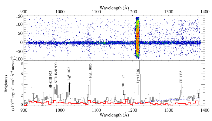
Figure 3.— Top – raw longslit far-UV spectrum from sounding rocket experiment 36.136 UG. Bottom – total nebular brightness per Å summed over the whole slit, excluding the continuum source. The red line is the estimated detector background. There is no significant dust scattering or H₂ continuum fluoresence emission above this background. The rise longward of Ly$\alpha$ is likely caused by 2s – 1s, 2-photon emission of recombining hydrogen. The dotted blue line shows the expected brightness for a column of $N(2s)$ = 4 $\times$ 10⁸ cm^-2.

Observations by Huggins et al. (1996) of the CO(2–1) 230 GHz emission lines at a position 68$\arcsec$W and 63$\arcsec$S from the CS also exhibit similar double peaked line profiles, with a total separation $\approx$ 30 km s^-1. At this position they estimate a CO column density of 6.9 $\times$ 10¹⁵ cm^-2 (assuming LTE with 5 $<T_{ex}<$150 K). At a position 10″ due West of the CS, Bachiller et al. (2000) show lines split by 53 $\pm$ 1 km s^-1(their Figure 4), yielding an expansion velocity of $\approx$ 27 km s^-1 with symmetry about a heliocentric velocity of –43 km s^-1(at M27, $V_{hel}$ = $V_{lsr}$ – 17.8 km s^-1), in good agreement with the Wilson systemic velocity. They present a map of the region (beam size 12″), showing the CO emission to be clumpy and more-or-less coincident with the molecular hydrogen infrared emission observed by Kastner et al. (1996). Bachiller et al. (2000) present a picture of an ionized central region with an electron density of about $n_{e}\sim$ 100 cm^-3 surrounded by a ring of molecular clumps with densities $\sim$ 10⁴ cm^-3 undergoing photodissociation. They suggest the clumps are similar to the “cometary” shaped features observed in great detail in the Helix nebula (c.f. O’Dell et al., 2002; Huggins et al., 2002; Meixner et al., 2005), although the cometary morphology is not as prominent in the Dumbbell as it is in the Helix. Meaburn & Lopez (1993) first noted (see also HST images by O’Dell et al., 2002) that some clumps appear as dark knots against the very bright O III emission that surrounds the central region.

McCandliss (2001) gave a preliminary analysis of molecular hydrogen absorption in the FUSE spectra, identifing two absorption systems, one blueward of the CS radial velocity and one redward. The blueward component has lines originating from an excited electronic ground state ($X\,^{1}\Sigma_{g}^{+}$), with rotational levels ($J\arcsec$) up to 15 and vibrational levels ($v\arcsec$) at least as high as 3. Many lines originating from $v\arcsec$ = 1 and 2 are located longward of the ground state bandhead ($v^{\prime}$  – $v\arcsec$ = 0 – 0) at 1108.12 Å, and as such are unambiguous markers of “hot” H₂. In contrast, the redward component is much “cooler,” showing no unusual excitation (J${}^{\prime\prime}_{max}~{}\approx$ 4, $v\arcsec$ = 0). It is associated with non-nebular foreground gas. Here we will refine the original analysis, which was based on LWRS data acquired under FUSE PI Team Program P104.

Lastly we note, Ly$\alpha$ fluorescence of H₂ has recently been found in the PNe M27 and NGC 3132 by Lupu et al. (2006). The fluorescence is a direct consequence of excited molecular hydrogen, as the mechanism requires a significant population in the $v\arcsec$ = 2 levels in the presence of strong Ly$\alpha$ emission. Herald reports (private communication) that FUSE observations of the CS of NGC 3132 also exhibit excited H₂ absorption lines with a roughly thermal ro-vibrational distribution of $\approx$ 1750 K.

3. Datasets

3.1. FUSE

A description of the data set and processing procedures for the FUSE spectra of the CS (MAST object ID GCRV12336) used in this study can be found in McCandliss & Kruk (2007). For a description of the detectors, channel alignment issues, systems nomenclature and other aspects of the FUSE instrument, see Moos et al. (2000) and Sahnow et al. (2000). Briefly, the CS was observed numerous times for observatory wavelength calibration purposes. High signal-to-noise spectra, acquired in time tag mode through the high resolution slits (HIRS) of the eight different channel segments have been assembled. Data for each extracted channel segment consists of three 1-D arrays: wavelength (Å), flux (ergs cm^-2 s^-1 Å^-1), and an estimated statistical error (in flux units). Figure 1 shows the eight individual channel segments and their spectral range for all the coadded HIRS spectra. The high density of the H₂ features is apparent.

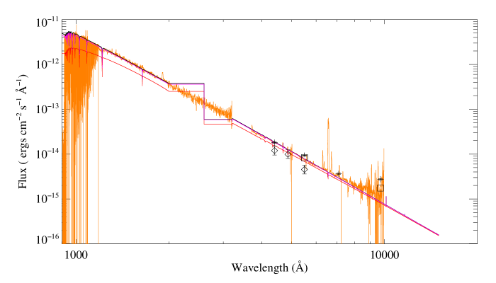
Figure 4.— Log-log plot of the M27 central star SED from 900 - 20000 Å, as measured by FUSE, IUE, APO and the optical photometry of Tylenda et al. (1991) ($\diamond$), (Ciardullo et al., 1999) (□) and Benedict et al. (2003) (+). Overplotted in black, purple and red are the respective unextinguished, lightly extinguished ($E(\bv)$ = 0.005) and heavily extinguished ($E(\bv)$ = 0.05) stellar continuum models. Break between 2000 and 3000 Å indicates a gap in the stellar model.

In the low sensitivity SiC channels the continuum signal-to-noise is between 10 – 25 per pixel, while in the higher sensitivity LiF channels it is 20 – 55. These signal-to-noise ratios are purely statistical and do not account for systemic errors, such as detector fixed pattern noise. The resolution of the spectra changes slightly as a function of wavelength for each channel segment. In modeling the H₂ absorption (§ 4.1), we find that a gaussian convolution kernel with a full width at half maximum of 0.056 Å at 1000 Å (spectral resolution $R$ $\approx$ 18,000, velocity resolution ${\delta}V$ $\approx$ 17 km s^-1) provides a good match to the unresolved absorption features throughout most of the FUSE bandpass.

Close comparison of the wavelength registration of overlapping segments reveals isolated regions, a few Å in length, of slight spectral mismatch ($\sim$ a fraction of a resolution element) in the wavelength solutions. Consequently, combining all the spectra into one master spectrum will result in a loss of resolution. However, treating each channel/segment individually increases the bookkeeping associated with the data analysis. Further, because fixed pattern noise tends to dominate when the signal-to-noise is high, there is little additional information to be gained in analyzing a low signal-to-noise data set when high signal-to-noise is available. For these reasons we elected to form two spectra, each of which covers the 900 – 1190 bandpass contiguously, using the following procedure.

The flux and error arrays for the LiF1a and LiF1b segments were interpolated onto a common linear wavelength scale with a 0.013 Å bin, covering 900 – 1190 Å. The empty wavelength regions, being most of the short wavelength region from 1000 Å down to the 900 Å and the short gap region in between LiF1a and LiF1b, were filled in with most of SiC2a and a small portion of SiC2b respectively. We refer to this spectrum as s12. The LiF2b, LiF2a, SiC1a and SiC1b segments were merged similarily into a spectrum, s21. Absorption line analyses were carried out using the composite s12 and s21 spectra (§ 4.1).

3.2. Far-UV Longslit Observations of M27 from JHU/NASA Sounding Rocket 36.136 UG

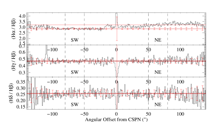
Figure 5.— Long slit profiles of H$\alpha$/H$\beta$, H$\beta$/H$\gamma$, and H$\beta$/H$\delta$. Intrinsic line ratio for a gas with a temperature of 10000 K and a density of 100 cm^-3 is overplotted in black. The data have been binned up by two 0$\farcs$4 pixels. Average values in the SW and NE region, delimited with the vertical dashed lines, are overplotted in red. Error bars are displayed with respect to the average in the SW region. All the ratios are consistent with zero extinction except for the NE H$\alpha$/H$\beta$ ratio. This result suggests that a mechanism, other than extinction by dust, is causing the H$\alpha$/H$\beta$ ratio to deviate from the expectations of recombination.

JHU/NASA sounding rocket mission 36.136 UG was launched from White Sands Missile Range Launch Complex-36 on 14 June 1999 at 01:40 MST. Its purpose was to observe the hot CS of M27, provide spatial information on the excitation state of H₂ in the nebula and investigate its dust scattering properties. The science instrument was a 40 cm diameter Dall–Kirkham telescope with SiC over-coated Al mirrors, feeding a Rowland circle spectrograph with a 200″ x 12″ longslit, a 900 – 1400 Å bandpass and an inverse linear dispersion of $\approx$ 20 Å mm^-1. The basic configuration has been described by McCandliss et al. (1994); McCandliss et al. (2000) and Burgh et al. (2001) and two similar missions using this payload have flown (Burgh et al., 2002; France et al., 2004). This was the first flight for a newly reconfigured spectrograph with a holographically corrected concave grating (McCandliss et al., 2001), for improving the spatial resolution (3″ spacecraft pointing limited) and a high QE KBr coated micro-channel plate with double-delay line anode ($\approx$ 25 $\mu$m resolution element), similar to that used by McPhate et al. (1999).

The target was acquired at $\approx$ T+150 s, at which time pointing control was passed to a ground based operator, who used a live video downlink of the nebular field to make real time pointing maneuvers. At $\approx$ T+500 s the telescope was sealed prior to reentering the atmosphere. The payload was recovered and post flight calibrations were made to secure an absolute calibration.

The pointing corrected two dimensional spectrum is shown in the top panel of Figure 3. C II $\lambda$1335, C III $\lambda$977 and $\lambda$1175, He II+N II $\lambda$1085, N III $\lambda\lambda$989 – 991 and H I Lyman emission lines are evident along with the continuum spectrum of the central star. The bottom panel shows the extracted nebular spectrum integrated over the length of the slit, excluding the stellar continuum. The strong Ly$\alpha$ emission feature that fills the slit is dominated by geocoronal emission. There is a hint of H I 2s – 1s two photon emission starting at Ly$\alpha$ and rising towards 1400 Å. The dotted blue line shows the expected brightness for an column of $N(H(2s))$ = 4 $\times$ 10⁸ cm^-2 (e.g. Nussbaumer & Schmutz, 1984). There is no evidence for continuum pumped fluorescence of H₂ or dust scattered stellar continuum down to the detector background limit of $\approx$ 5 $\times$ 10^-17 ergs cm^-2 s^-1 Å^-1 arcsec^-2  indicated by the red line.

Figure 6.— Nearest neighbor H I 21 cm emission spectra from the Dwingloo spectral survey atlas. These spectra were used to form a minimum spectrum and a distance-weighted mean spectrum.

Figure 7.— Top – Minimum spectrum is subtracted from the angular distance weighted mean spectrum to remove wide angle background emission. Vertical axis is column density per km s^-1. Horizontal axis is heliocentric velocity. Bottom – Resulting spectrum contains both foreground and some background emission. Nine component gaussian fit is shown along with the fit residuals (offset by -5 $\times$ 10¹⁸ cm^-2). See Table 2 for total columns, velocity centroids, and doppler parameters derived from gaussian fits.

3.3. APO DIS Longslit Observations of Balmer Line Ratios in M27

It is curious that Hawley & Miller (1978) and Barker (1984) both cited problems with their $H{\alpha}$/$H{\beta}$ ratios being higher than the 2.9 ratio determined by Miller (1973). Hawley & Miller (1978) suggested some unidentified systematic error was affecting the ratio at the 10% level. Barker (1984) reached a similar conclusion and went so far as to decrease the $H{\alpha}$/$H{\beta}$ by 13% before applying an extinction correction of $c$ = 0.17. Both studies find $\approx$ 20% variations in $H{\alpha}$/$H{\beta}$ at different locations within the nebula.

To more thoroughly investigate this phenomenon we recently acquired an extensive series of longslit spectral scans of the nebula with the Double Imaging Spectrograph (DIS version III) at the ARC 3.5 m telescope at Apache Point Observatory (APO), during the nights of 1 – 2 July 2006 commencing at 01:15 MDT. DIS has blue and red spectra channels with back-illuminated, 13.5 $\mu$m pixel Marconi CCDs in a 1028 $\times$ 2048 pixel² format for recording data. The medium resolution gratings have inverse linear dispersions of 1.85 and 2.26 Å pixel^-1 respectively. The useful spectral ranges are 3700 – 5400 Å for the blue and 5300 – 9700 Å for the red. The plate scales are 0$\farcs$42 pixel^-1 for the blue and 0$\farcs$40 pixel^-1 for the red.

The hot sub-dwarf star BD +28 4211 was used as a spectrophotometric standard (Bohlin et al., 2001). This star was observed through the large 5″ $\times$ 300″ DIS slit for 60 seconds at an airmass of 1.18. The M27 CS was observed shortly thereafter for 200 seconds through the same aperture at an airmass of 1.02. The CS and surrounding nebula were then observed through the narrowest 0$\farcs$9 $\times$ 300″  DIS slit for 200 seconds, with the slit held fixed on the CS. The narrowest slit provides clean separation of the [N II] $\lambda\lambda$6548, 6584 lines from $H{\alpha}$. The position angle of the slit was 35°. Biases, flat fields and emission line spectra were recorded at twilight. and the data were reduced using custom IDL code. The CS absolute flux is shown in Figure 4 and will be discussed in § 4.2. The Balmer line longslit profiles centered on the CS, and ratioed to $H{\beta}$, are shown in Figure 5 and will be discussed in § 4.2.1. Analysis of the full dataset from the APO run will be presented elsewhere.

3.4. Dwingeloo H I 21-cm Observation of M27

The shapes of atomic hydrogen absorption profiles are complex, as they result from ensembles of intervening ISM absorption systems, separated in velocity space along the line-of-sight. Determining the column density and doppler parameter for individual velocity components within these broad damped and saturated absorption profiles is difficult without a priori information of the line-of-slight velocity structures. One way to gain this information is to examine H I 21 cm emission data such as found in the Atlas of Galactic Neutral Hydrogen (Hartmann & Burton, 1997, also known as the Dwingeloo survey). The high spectral resolution of the data is excellent for locating velocity components, provides an upper limit to the amount of neutral hydrogen in the foreground, and serves as a starting point for absorption line modeling. The atlas, in galactic coordinates ($l,b$) with (0$\fdg$5)² cells, has a velocity spacing of 1.03 km s^-1. The positions cover most of the sky and the velocity coverage spans –450 $\leq$ v_lsr $\leq$ 400 km s^-1 in local-standard-of-rest coordinates. The intensity is given in antenna temperature per velocity (K (km s^-1)^-1), but can be converted to a H I column density, under the assumption of optically thin emission, by multiplying with a conversion factor (0.182 $\times$ 10^-19 cm^-2, Hartmann & Burton, 1997).

The galactic coordinates of M27 are $l$ = 60$\fdg$84, $b$ = –3$\fdg$70. The neutral portion of the nebula should be at least as large as the H$\alpha$ halo detected by Papamastorakis et al. (1993) ($\gtrsim$ 0$\fdg$28) and since the Dwingeloo half power beam width is slightly larger than the atlas grid, it is reasonable to expect some signal from the nebula to appear in the four nearest neighbor points, i.e. atlas coordinates ($l$ = 61$\fdg$, $b$ = –3$\fdg$5) ($l$ = 60$\fdg$5, $b$ = –3$\fdg$5) ($l$ = 61$\fdg$, $b$ = –4$\fdg$) and ($l$ = 60$\fdg$5, $b$ = –4$\fdg$). The column density profiles of H I as a function of velocity for these four grid points, in heliocentric velocity coordinates, are shown in Figure 6.

To reduce the non-local contributions we constructed a nearest neighbor minimum spectrum under the assumption that non-local contributions are widespread and uniform. This assumption has been checked by examining an area out to $\pm$1$\fdg$5, which showed similar structures, typified by strong peaks near 0 km s^-1 and smaller peaks near -85 km s^-1. The nearest neighbor minimum spectrum was smoothed with a five bin boxcar average and subtracted from a similarily smoothed spectrum formed from a distance weighted average of the same 4 nearest neighbors. This process is shown in Figure 7. The resulting subtraction was fit with nine Gaussian profiles spread between –99 $<v_{hel}<$ 24 km s^-1. The integrated emission column densities, rms velocity widths (b values), and heliocentric velocities are given in columns 2, 3, and 4 of Table 2.

Column 5 shows the column densities that we adopted for the model of the Lyman series absorptions as discussed in § 4.3. Absorption line components to the blue of the systemic velocity at –42 km s^-1 occur within the expansion velocity inferred from the optical emission lines and can plausibly be associated with the nebular expansion. If the absorption components to the red of –42 km s^-1 are associated with the nebula they would have to be infalling. They are more likely to be located in the foreground.

3.5. STIS

The E140M spectrum of M27 (o64d07020_x1d.fits), taken from the Multimission Archive at Space Telescope (MAST), was acquired for HST Proposal 8638 (Klaus Werner – PI). These data are a high level product consisting of the extracted one-dimensional arrays of flux, flux error and wavelength for the individual echelle orders. The data were acquired through the 0$\farcs$2$\times$0$\farcs$2 spectroscopic aperture for an exposure time of 2906 s and were reduced with CALSTIS version 2.18. The spectral resolution of the E140M is given in the STIS data handbook (version 7.0 Quijano, 2003) as $R$ $\approx$ 48,000 (${\delta}V$ = 6.25 km s^-1). The intrinsic line profile for the 0$\farcs$2$\times$0$\farcs$2 aperture has a gaussian core with this width, but there is non-negligible power in the wings. Comparison of the FUSE and STIS wavelength scales for the CS revealed a discrepant offset. The establishment of a self consistent wavelength scale is discussed in § 4.5.

4. Data Analysis

Our primary purpose is to quantify the excitation state of the H₂ in the diffuse nebular medium. The column densities of the individual ro-vibrational states were determined using curve-of-growth analysis. We detect essentially imperceptible reddening of the stellar SED over a decade of wavelength coverage, in contrast to the reddening determinations using the Balmer decrement method as reported in the literature (§ 2). We show new high precision longslit Balmer decrement ratios (H$\alpha$/H$\beta$, H$\gamma$/H$\beta$, and H$\delta$/H$\beta$) where H$\alpha$/H$\beta$ appears to be reddened in certain regions of the nebula, but the higher order decrements appear unreddened everywhere. A potential resolution of the reddening conundrum will be discussed in § 5.4.

We also produce an estimate of the total atomic hydrogen column density in the nebula to enable a discussion of H₂ formation and destruction processes. An upper limit is placed on the column density of CO in the diffuse medium and an analysis of the excitation of C I fine structure lines will provide a diagnostic of nebular pressure and insight into the H₂ exitation mechanism. Absorption line profiles of high and low ionization species compared to the neutral profiles reveal the ionization stratification of the outflow and provide a velocity description of the nebular kinematics.

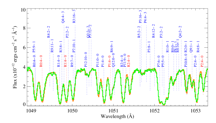
Figure 8.— Region near the H₂ (4–0) band identifying the high excitation velocity component at –33 km s^-1 (blue) and the low excitation component at +14 km s^-1 (red) as measured in the CS restframe. FUSE s12 and s21 spectra are overplotted in orange and green respectively.

Figure 9.— Upper – curves-of-growth for doppler parameters of 6 and 7 km s^-1 along with the data. A doppler parameter of 6.5 km s^-1 was adopted. Lower – column densities, normalized by level statistical weight, as a function of the level energy. The $v\arcsec$ = 0, 0 $\leq J^{\prime\prime}\leq$11 columns are shown with + marks, and the $v\arcsec$ = 1, 0 $\leq J^{\prime\prime}\leq$11 columns are shown with * marks. Overplotted (solid line) is a single temperature Boltzmann distribution for $T$ =2040 K. There are statically significant deviations from the single temperature population, although the higher 7 $\leq J^{\prime\prime}\leq$ 11 states are in agreement. The lower 0 $\leq J^{\prime\prime}\leq$ 6 states appear to have a flatter slope indicative of a temperature a factor of two higher as the dashed lines indicate.

4.1. Curve-of-Growth for the Molecular Hydrogen Absorption Components

It seems with a first glance at Figure 1 that determining the column densities for the ro-vibrational transitions and identifying velocity components will be daunting. However, the regular spacing of H₂ lines arising from common rotational states, along with the monotonic variation in transition strength with increasing upper vibrational level, makes identification of discrete velocity components straightforward. The high line density becomes an advantage, virtually guaranteeing a few lines for a given rotational state will be unblended. This allows column densities to be determined by a straight forward measurement of the equivalent widths for use in a curve-of-growth analysis.

We have identified two distinct components with heliocentric velocities of –75 and –28 $\pm$ 2 km s^-1. The blueward velocity component is the more highly excited, allowing the construction of curves-of-growth for all the ro-vibrational levels with $J\arcsec$ $\leq$ 11 and $v\arcsec$$\leq$ 1 of the ground electronic state $X\,^{1}\Sigma_{g}^{+}$. The redward component has no extraordinary excitation with measurable absorption only found for $J\arcsec$  $\leq$ 3 in $v\arcsec$ = 0. Figure 8 shows a small region around the ($v^{\prime}$–$v\arcsec$) = (4–0) band near 1050Å where the “blue” and “red” velocity components are identified. Blueward absorptions for ($v^{\prime}$–1), ($v^{\prime}$–2) and ($v^{\prime}$–3) in this region are also displayed.

A semi-autonomous method was developed to measure the equivalent widths of the lines, based in part on the completely autonomous method used by McCandliss (2001). All the lines for a given velocity offset and rotational state were located within a summation interval initially 13 – 15 pixels wide. The pixels adjacent to either side of the summation interval were used to define continuum points, through which a straight line was fit to serve as the model for the continuum in the summation region. The degree of blending was assessed interactively by plotting the spectrum surrounding each individual line in a (-150, 50) km s^-1 interval and overplotting all the known atomic and molecular features. Lines with evidence of blending were rejected from the curve-of-growth. Examination of the lines for blends provided an opportunity to fine-tune the summation interval and continuum placement. The equivalent width measurements were carried out on both the s12 and s21 spectra (see § 3.1), using the same summation and continuum intervals. Allowance was made for the slight local mismatches in velocity scale that exist between the s12 and s21 spectra, by locating the minimum within the integration region and adjusting the interval accordingly.

Initial curves-of-growth were constructed from the equivalent width measurements using the wavelengths and oscillator strengths from Abgrall et al. (1993a, b). We required at least 2 unblended lines for these curves. Lines from transitions with $J\arcsec$  $\geq$ 11 and $v\arcsec$ $\geq$ 2 are detected, but they are weak and too few to construct a reliable curve-of-growth. Independent $\chi^{2}$ fittings were performed for each curve by varying the doppler parameter over 2 – 10 km s^-1 and the logarithm of the column density (in cm²) over 13 – 18 dex. The doppler parameters thus derived varied from 4 to 8 km s^-1 and the logarithmic column densities ranged over $\approx$ 13.5 – 17 dex.

Table 1Derived Nebular H₂ $X\,^{1}\Sigma_{g}^{+}$ Column Densities

J′′	$\log{N(v^{\prime\prime}=0)}$	ncog	$\log{N(v^{\prime\prime}=1)}$	ncog
	$\log$(cm-2)	lines	$\log$(cm-2)	lines
0	15.0	2	13.6	3
1	15.9	11	14.4	5
2	15.7	8	14.2	3
3	16.3	4	14.6	9
4	15.8	4	14.1	10
5	16.4	8	14.6	12
6	15.7	8	14.1	5
7	15.8	5	14.5	11
8	15.2	7	13.9	2
9	15.2	11	14.3	4
10	14.6	13	13.5	2
11	14.8	5	13.8	2

Comparing results from the s12 and s21 measurements revealed a few disagreements for the doppler parameter (and thus column density) derived for the same rotational state. This produced an inconsistent modulation in the ortho-para ratio, expected to be $\approx$ 3:1 for the odd to even rotational states. The inconsistencies were traced to curves-of-growth with the most saturated lines and lowest number of points. Restricting the allowed doppler parameters in the fit to either 6 or 7 km s^-1 (the most common values) resolved the column density discrepancy and resulted in consistent ortho-para modulation. It also reduced the scatter when all the curves-of-growth for the individual rotational states from the s12 and s21 spectral measurements were combined (top panel of Figure 9). The column densities for the individual ro-vibrational levels are listed in Table 1 along with the number of lines used for each curve-of-growth. The errors are dominated by placement of the continuum. Experiments were performed to gauge the effect of systematic continuum offsets on the derived column densities. We found the column densities were consistent to within $\pm$ 0.1 in the dex for offsets within the local continuum signal-to-noise.

The total column density for the hot H₂ component at –75 km s^-1 is N(H₂)=7.9 $\pm$ 2 $\times$ 10¹⁶ cm² with a doppler velocity of 6.5 $\pm$ 0.5 km s^-1. Curve-of-growth analysis on the cold non-nebular component, for which we wish only to identify the strength of its aborption features, yielded a total column density of 1.3 $\pm$ 5 $\times$ 10¹⁷ cm² with a doppler velocity of 5 km s^-1. The rotational distribution is well approximated with a temperature of 200 K.

In the bottom panel of Figure 9 we show the population density of the ro-vibrational levels as a function of level energy. We use (+) marks to indicate the columns for $J\arcsec$ in the $v\arcsec$ = 0 state and (*) marks to indicate the columns for $J\arcsec$ in the $v\arcsec$ = 1 state. The straight solid line is the best fit single temperature model ($T$ = 2040 K), assuming a Boltzmann distribution of level populations. This model is not successful, as there are statistically significant deviations from a single temperature Boltzmann destribution.

The variation of population density as a function of level energy is quite different from what is usually observed in the cold ISM. Typically the first two rotational levels are consistent with a rather steep slope with a temperature $T_{01}\sim$ 80 K while the higher rotational levels flatten, giving the appearance of a higher “temperature” of several hundred degrees or more (Spitzer & Cochran, 1973). The excess column in the $J>$ 1 levels has long been thought to be caused by far-ultraviolet continuum fluoresence, but recently Gry et al. (2002) has questioned this hypothesis. They favor a true two temperature model for the ISM.

Regardless, here we have the opposite case. In each vibrational level $v\arcsec$ = 0, 1 the trend is for the lower rotational states to have flatter slopes (higher temperature) than the higher rotational states. Reproduction of the energy level distribution found here will be an interesting challenge for H₂ excitation models (c.f. Spitzer & Zweibel, 1974; Black & Dalgarno, 1976; Shull, 1978; van Dishoeck & Black, 1986; Sternberg & Dalgarno, 1989; Draine & Bertoldi, 1996). We note how the modeling by Spitzer & Zweibel (1974) shows qualitatively how the “curvature” of the population density can go from “concave” to “convex” as the parameters change from a low temperture, density and photoexcitation rate environment to either a high photoexcitation rate or a high density environment. However, they do not attempt to explore temperatures in excess of 1000 K.

4.2. Central Star Spectral Energy Distribution and Extinction

SED models with CS parameters taken from the literature provide a fairly precise match to the stellar continuum observed by FUSE. This allows us to determine the line-of-sight extinction, and provides a reasonable stellar continuum to use for assessing the success of our model of atomic and H₂ absorption. The combined SED and absorption model has been used by McCandliss & Kruk (2007) to identify 63 photospheric, nebular and non-nebular absorption features of ionized and neutral metals, lurking amid the sea of hydrogen features.

In Figure 4 we show a log-log plot of the CS SED from 900 – 20000 Å, as measured using FUSE, IUE, and the APO DIS, along with the optical photometry (Tylenda et al., 1991; Ciardullo et al., 1999; Benedict et al., 2003). Over-plotted is a synthetic stellar flux interpolated from the grid of Rauch (2003) with $\log{g}$ = 6.5, T = 120,000 K, and ratio of H/He = 10/3 by mass. This model includes no metals and is consistent with, although slightly hotter than, the quantitative spectroscopy of Napiwotzki (1999). It is slightly cooler than the determination of Traulsen et al. (2005). The temperature and gravity adopted for our model has slightly less pressure broadening and is a better match to the observed Lyman lines towards the series limit. We also adopt a stellar mass of 0.56 $M_{\sun}$ as suggested by post asymptotic giant branch evolutionary tracks.

Use of this mass along with the above gravity required a distance of 466 pc to match the absolute flux, which is at the upper limit given by Benedict et al. (2003). Beyond our immediate need to match the absolute flux for the given gravity and mass there is no particular reason to prefer this distance over that derived by Benedict et al.. Questions regarding the acceptable uncertainty in distance, absolute flux and derived stellar parameters are best left for a stellar model specifically tailored to include the effects of metals, gravity and evolutionary state. For our purpose, the high stellar temperature places the SED longward of the Lyman limit in the Rayleigh–Jeans regime, so the shape of the SED is insensitive to our assumptions of temperature, gravity, metallicity, mass and distance. Consequently, long-range changes in SED shape produced by reddening can be constrained with a high degree of confidence.

The model flux is shown in Figure 4 with reddenings of E(B V) = 0.00, 0.005 and 0.05 assuming the R_V = 3.1 curve of Cardelli et al. (1989). An extinction of E(B V) = 0.05 is clearly too high. As a convenience we adopt a very modest extinction of E(B V) = 0.005, as seen most clearly in Figure 1 to make the continuum towards the Lyman edge match the stellar SED. The lack of any significant extinction is roughly consistent with the total nebular hydrogen, derived in § 4.3, and the standard conversion for color excess to total hydrogen column of $N(H)/E(\bv)$ = 5.8 $\times$ 10²¹ cm^-2 mag ^-1 (Bohlin et al., 1978).

4.2.1 Balmer Line Reddening

Reddening by dust in PNe is often estimated by comparing the measured Balmer emission ratios to the intrinsic ratios produced by hydrogen recombination. The intrinsic intensity ratio (in flux units) of $I(H\alpha)$/$I(H\beta)$ $\simeq$ 2.859 at an electron temperature of 10⁴K and density of 10² cm^-3, is accurate to within $\approx\pm$ 5% for a wide range of the electron temperature and density, (5000 $<T_{e}$(K) $<$ 20000, 10${}^{2}<N_{e}($cm${}^{-3})<$ 10⁶) (Brocklehurst, 1971). The extinction parameter $c$ is given in

$$I(\lambda)/I(H\beta)=F(\lambda)/F(H\beta)10^{cf(\lambda)}$$ (1)

where the intrinsic ratio is $I(\lambda)/I(H{\beta})$, the observed ratio is $F(\lambda)/F(H{\beta})$ and $f(\lambda)$ is the line attenuation, relative to H$\beta$, at any wavelength for the given extinction curve (c.f. Miller & Mathews, 1972; Cahn, 1976). The extinction parameter may be converted to selective extinction by adopting the ratio of $c/E(\bv)$ = 1.5 as shown by Ciardullo et al. (1999) in their Figure 5.

Balmer emission line spatial profiles for H$\alpha$, H$\beta$, H$\gamma$, and H$\delta$ in a $\pm$ 140″ region to either side the CS at a position angle of 35 $\arcdeg$, were acquired as discussed in § 3.3. The line ratios, with respect to $H\beta$, are displayed in Figure 5 with a two pixel (0$\farcs$9) binning. The reddenings derived from these ratios (Figure 5) are inconsistent and are summarized in Table 3. The first column specifies the line ratio, the second is the extinction multipler taken from Barker (1984), the third is the intrinsic line ratio for a temperature of 10,000 K and a density of 100 cm^-3 taken from Brocklehurst (1971), the fourth and fifth columns are the average line ratios and standard deviations for the SW and NE regions after rebinning the data by sixteen pixels (7$\farcs$2), and the sixth and seventh columns are the derived selective extinctions and associated errors. The NE H$\alpha$/H$\beta$ ratio suggests $E(\bv)$ = 0.10 $\pm$ 0.02, while all the rest of the ratios are consistent with much lower or no extinction.

The line ratio averages in the fiduical SW and NE regions have standard deviations of 1.5 – 3 % after rebinning by sixteen pixels. The large error bars in the derived $E(\bv)$ serve to emphasize that Balmer line ratio determinations to a precision of better than 1% are required for $E(\bv)<$ 0.01. We note that in the immediate vicinity of the star H$\alpha$/H$\beta$ = 3.03 yielding $E(\bv)$ = 0.051, which is much too large to be consistent with the observed far ultraviolet SED (see § 4.2), assuming the line-of-sight extinction is close to the Galactic standard.

We concluded in the previous section that dust along the diffuse line of sight produces $E(\bv)\leq$ 0.01 mag. Here we find the extinction in the extended medium is low to nonexistent. We conclude that dust is not widespread, although it may be confined to the clumpy medium. The inconsistancies in Balmer reddening measures suggest that a process other than extinction by dust is contributing to H$\alpha$/H$\beta$ ratio excess. We will discuss this issue further in § 5.4.

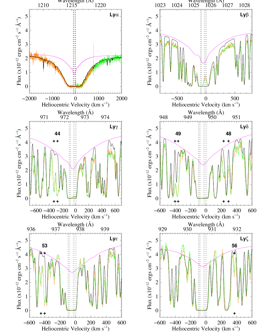
Figure 10a.— Lyman series model fits (Ly$\alpha$ – $\mu$). The long dashed lines near the center of the profiles mark the velocities of the absorption components determined from the Dwingeloo data. In Ly$\alpha$ the two STIS E140M orders are shown in orange and green. The FUSE data are shown as orange (s12) and green (s12). The stellar continuum is in purple and the absorption model is in black. The numbered +’s mark absorption features tabulated in Table 2 of McCandliss & Kruk (2007).

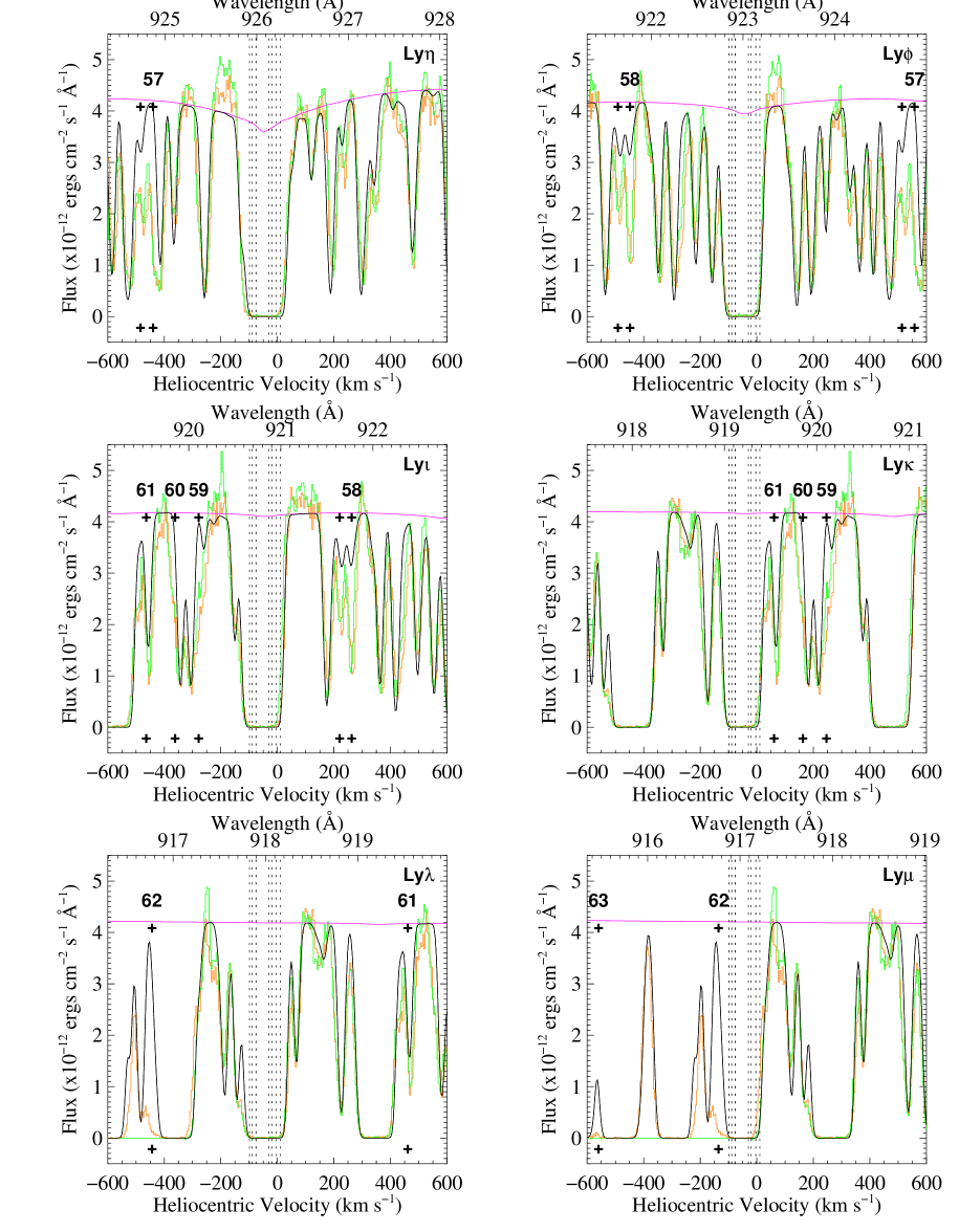
Figure 10b.— Lyman series model fits (Ly$\eta$ – $\mu$). Colors and marks are the same as in Figure 10a.

4.3. Atomic Hydrogen Absorption Model

Table 2H I 21 cm Velocity Component Column Densities

Component	$\log{N_{em}}$	$b$	$V_{hel}$	$\log{N_{abs}}$
	$\log$(cm-2)	(km s-1)	(km s-1)	$\log$(cm-2)
1	19.0	2.9	-98.5	18.9
2	19.3	3.4	-88.7	19.0
3	19.6	5.3	-75.3	19.0
4	19.7	20.4	-75.7	18.2
5	19.4	5.3	-29.9	19.4
6	19.2	2.6	-20.0	19.2
7	20.3	6.2	-3.5	19.3
8	20.4	4.3	10.7	18.0
9	19.7	7.5	23.6	$\cdots$

Table 3Extinctions Derived from Balmer Ratios

	$f(\lambda)$	Int Ratio	Obs Ratio SW	Obs Ratio NE	$E(\bv)$ SW	$E(\bv)$ NE
$\frac{H\alpha}{H\beta}$	-0.33	2.859	2.868 $\pm$ 0.041	3.205 $\pm$ 0.066	0.003 $\pm$ 0.013	0.100 $\pm$ 0.018
$\frac{H\gamma}{H\beta}$	0.15	0.4685	0.4627 $\pm$ 0.0093	0.4724$\pm$ 0.0144	0.024 $\pm$ 0.039	-0.016$\pm$ 0.059
$\frac{H\delta}{H\beta}$	0.20	0.2591	0.2585 $\pm$ 0.0075	0.2508$\pm$ 0.0082	0.003 $\pm$ 0.042	0.047 $\pm$ 0.048

In Table 2 we list the column densities, doppler velocities and heliocentric velocity offsets inferred from the Dwingeloo data (§ 3.4). The 21-cm emission column densities listed in column 2 have contributions from both background and foreground emission, so they provide an upper limit to the expected foreground absorption column densities. We are mostly concerned with finding reasonable numbers for the nebular absorption, i.e. those components shortward of the stellar systemic velocity of –42 km s^-1; components 1 – 4. We will refer to components 5 – 9 as the non-nebular ISM components.

The adopted neutral hydrogen absorption model, the components of which are listed in column 5, was determined with the following procedure. We initially allowed the two components nearest to $V_{sys}$ (5 and 6) to retain the maximum column suggested by the emission line fit. The two components nicely filled the centers of the Ly$\alpha$ – Ly$\mu$ lines. We then moved to the blueward side and reduced the column of component 1 until a good agreement was found in the most saturated lines Ly$\eta$ – Ly$\mu$. We continued to add in components 2, 3 and 4 reducing the columns as necessary to smoothly match the absorption in the saturated lines. Once we were satisfied with the blue edge fit we proceeded to the redward components. It was determined that component 9 produced too much red edge absorption in all the Lyman series lines and it was eliminated from further consideration. We found that only a modest amount of component 8 was necessary to match the redward edge of Ly$\alpha$. Finally component 7 was added to reduce the absorption gap between components 6 at –20 km s^-1 and 8 at 11 km s^-1. Changing the column density of any one component by the error in the emission line fit (0.15 dex) did not appreciably cause deviations of the resulting model with the data. The constraints on the formation and destruction of molecular hydrogen within the nebula, which we discuss in § 5.3, are immune to the details of the velocity distribution of H I derived from the Dwingeloo data.

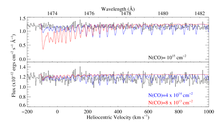
Figure 11.— HSTSTIS E140M spectrum of the region around CO A–X (2–0), the strongest band in the A–X absorption series. Top – Two different excitation temperature models (3000 K, blue) and (300 K,red) of the (2–0) band using the same column, 10¹⁵ cm^-2, as suggested from CO mm measurements. Bottom – noise bounded upper limits to the line-of-sight CO column for the two excitation temperatures. Note the scale change between the two panels. The upper limit drops for decreasing excitation temperatures, because the population becomes concentrated in the lower rotational levels as temperature decreases.

Figure 10a shows an overlay of the adopted atomic and H₂ absorption model on the Ly$\alpha$ – Ly$\mu$ lines from STIS and FUSE. The Ly$\alpha$ profile from the STIS E140M observation spans two orders, plotted as orange and green. The rest of the Lyman series are from FUSE with the s12 spectrum shown in orange and s21 shown in green. The stellar SED is shown in purple and the model is in black. The locations of the the individual H I velocity components from Table 2 are marked with vertical dotted lines. The model includes the H₂ absorption determined in § 4.1. A comparison of the hydrogen absorption model against the s12 and s21 spectra for the entire FUSE wavelength range along with metallic absorption system identifications, arising from the photosphere, the nebula and non-nebular ism, can be found in McCandliss & Kruk (2007). We see that the model continuum in the vicinity of Ly$\beta$ is $\sim$ 10% too high, while at the shortest wavelengths it is low by a similar amount. There are also indications of absorption from O I and N II features (McCandliss & Kruk, 2007, Table 2).

Although the agreement of the model with the data is excellent, the procedure adopted here for constraining the neutral hydrogen column in the nebula is not ideal and in all likelihood provides a non-unique solution. However, the result is at least plausible, well within factors of two, given the uncertainty associated with the large background subtraction necessitated by the coarse angular resolution of the Dwingeloo data cube. A high angular resolution 21 cm mapping of the nebula would provide a more useful constraint on the velocity components, column densities and doppler widths associated with the nebula. We are mainly concerned with the total H I column density of the nebula rather than the individual components. The sum of components 1 – 4 is N(H I)_neb = 3.0 $\pm$ 1 $\times$ 10¹⁹ cm². The non-nebular components 5 – 8 total to N(H I)_non = 6.2 $\pm$ 1 $\times$ 10¹⁹ cm².

4.4. CO Upper Limit and the C I Pressure Diagnostic

Figure 12.— Model of the neutral carbon multiplet UV2 (smooth line) is overplotted on the observed HSTSTIS spectrum (histogram). The nebular C I, C I* and C I** lines are labeled. The cold non-nebular C I, C I* are not labeled but the absorption is evident. There is no non-nebular C I** component. The model SED continuum is the lower smooth line. It was increased by 10% to improve the fit. The $f1$ and $f2$ fractions are relatively insensitive to continuum adjustments.

Figure 13.— The ($f1,f2$) planes for the expected ratios of the column densities of the C I fine structure states, assuming (left panel) neutral hydrogen impactors and (right panel) ionized impactors. The curves are the loci of ($f1,f2$) ratios for different pressures at a constant temperature. The large numbers to the upper left of each curve are the logarithms of the temperature. The log of the pressure in units of $\log(n_{h}T)=\log(P/k)$ is printed for every other density point along the loci of points for each constant temperature curve. The region shown is centered on ($f1,f2$) = (0.386, 0.477). The box centered on this point is the error limit ($\sigma_{f1},\sigma_{f2}$) = (0.04, 0.04). Despite the large uncertainty there is nearly an order of magnitude difference in the pressure for the two limiting cases. The temperature for the ionized impactors is closer to that of H₂.

4.4.1 CO Upper Limits

Bachiller et al. (2000) presented a detailed contour map of the CO (2–1) emission in M27. The contours fall steeply towards the CS where, using the conversion factor suggested by Huggins et al. (1996), we estimate an upper limit for the CO column of 10¹⁵ cm^-2 along the line-of-sight. CO has a number of strong absorption bands in the far UV, such as the numerous A-X bands spread throughout the STIS E140M bandpass, and this column density would easily be detected. In Figure 11 we show the E140M spectral region surrounding the A-X (2-0) 1477.565 Å bandhead. In the top panel we overplot CO absorption models for representative excitation temperatures of 3000 K and 300 K at a column density of 10¹⁵ cm^-2 in blue and red respectively. We assumed the doppler parameter is the same as for H₂, 6.5 km s^-1. Clearly the column density is much lower than 10¹⁵ cm^-2. In the lower panel we show models for 3000 K with a column density of 4 $\times$ 10¹⁴ cm^-2 and for 300 K with a column density of 8 $\times$ 10¹³ cm^-2. The structure in the models is on the order of the noise in the observation, so we will use these values as the (excitation temperature dependent) upper limits for line-of-sight CO. Using a lower excitation temperature would yield an even lower the upper limit.

4.4.2 C I Fine Structure Pressure Diagnostic

Although CO was not detected we do detect excited C I, C I* and C I** multiplets in the E140M data with a velocity of -75 km s^-1, coincident with the velocity of the excited H₂. The level populations of the three fine structure levels in the ground of C I, assuming a long enough time has passed for equilibrium to be established, is a detailed balance of the de-excitation and excitation rates set by collisions of C I with other particles (the impactors – H I, He I, p, e^-, ortho-H₂, para-H₂) and the radiative decay rates of the fine structure levels. Jenkins & Shaya (1979) present a useful diagnositic for gas pressure based on the ratios of the column densities for $N_{CI*}$ and $N_{CI**}$ relative to the total column density $N_{tot}$= $N_{CI}$ + $N_{CI*}$ + $N_{CI**}$, (f1 = $N_{CI*}$/$N_{tot}$ and f2 = $N_{CI**}$/$N_{tot}$). The pressure is constrained by comparing the measured values of f1 and f2 against theoretical loci for $f1$ and $f2$ at variable temperature and density.

We determined $f1$ and $f2$ by $\chi^{2}$ fits to the absorption profiles of the C I $\lambda\lambda$1656.27 – 1658.12 UV2 multiplet using the Morton (2003) oscillator strengths. The result is shown in Figure 12. We determined a doppler parameter of $b$ = 4.5 km s^-1 and we find $N_{CI}$ = 3.0 $\pm$0.5 $\times$ 10¹³ cm^-2, $N_{CI*}$ = 8.5 $\pm$0.5 $\times$ 10¹³ cm^-2 and $N_{CI**}$ = 10.5 $\pm$0.5 $\times$ 10¹³ cm^-2, yielding ($f1,f2$) = (0.386, 0.477) $\pm$ 0.04.

The theoretical loci for $f1$ and $f2$ depend on the mix of impactors assumed. Jenkins & Tripp (2001) discuss three extremes: Case1 where all the impactors are neutral hydrogen, Case 2 where all the hydrogen is molecular and Case 3 where all the hydrogen is ionized. They find Case 2 and Case 1 to yield very similar loci in the $(f1,f2)$ plane. Using their code (kindly provided by Jenkins, private communication) we show the results for Case 1 (left) and Case 3 (right) in Figure 13. The crosshairs mark the ($f1,f2$) point and the figure ranges over the $\pm$ 0.04 error limits. Crosses mark the density at intervals of 0.1 dex. The log of the pressure, in units of $\log(n_{h}T)=\log(P/k)$, is printed for every density point along the loci of points for each constant temperature.

For the neutral case the (0.386, 0.477) point lies on the $\log(T)$ = 2.6 curve with a pressure of $\log{n_{h}T}$ = 5.9, while the ionized case has $\log(T)\approx$ 3.0 with a pressure of $4.9<\log{n_{h}T}<5.0$. The allowed range of pressure for the $\pm$ 0.04 error box in the neutral case is 5.7 $\lesssim\ \log{n_{h}T}<\infty$ and for the ionized case 4.8 $\lesssim\ \log{n_{h}T}<\infty$ with the $\infty$ density case being associated with the coldest allowable logarithmic temperature of $\approx$ 2.1 dex.

Figure 14.— O VI*, O V* and C IV* lines used to reconcile the FUSE and STIS wavelength offsets. O Ve $\lambda$1371.292 establishes the gravitational redshift zero point. O VIe and C IVe are observed by both FUSE and STIS. FUSE spectra s12 (orange), s21 (green) and the model (black) are plotted along with overlapping STIS orders (purple and grey), if available. Vertical dashed lines mark the transition, $V_{sys}$, $V_{gr}$ and non-nebular velocities at –75, –42, –37 and –28 km s^-1 respectively. Red lines near 0 km s^-1 and +190 km s^-1 in the respective C IVe and O VIe panels mark gravitational redshift of redward doublet member. O VIe wavelength discrepancy (–0.42 Å) with NIST is noted.

The coincidence of the C I velocity with the H₂ velocity argues that these two species are co-located. The $\sim$ 2000 K implied by the H₂  ro-vibrational distribution is closer to the temperature given by the ionized case than the neutral case. This suggests the excited C I and H₂ are located in a warm and electron rich medium with $n_{e}\sim$ 80 cm^-3. In this environment it may be possible for H₂ to form at the interface between the ionized medium and the PDR clumps by H + e^- $\rightarrow$ H^- + $h\nu$ followed by H + H^- $\rightarrow$ H₂ + e^- mechanism, (c.f. Aleman & Gruenwald, 2004; Natta & Hollenbach, 1998). We note that our total column density for the neutral carbon, $N_{CItot}$ = 2.2 $\times$ 10¹⁴ cm^-2 is $\sim$ 2 orders of magnitude higher than what is expected for $N_{CItot}$ in typical H II regions, as discussed in Appendix A of Jenkins & Shaya (1979). It is likely that the source of C I in the diffuse medium is CO dissociation in the clumpy medium.

In addition to UV2, we also examined the fits for the UV3, UV4 and UV5 multiplets. We found that the $\chi^{2}$ fits to these multiplets yielded slightly different results. In the cases of UV3 and UV5, there were intervening unidentified absorption features that caused the $\chi^{2}$ to drift to higher columns for the $N_{CI**}$ lines. In the case of UV4 the column densities were different but the $f1$ and $f2$ ratios were essentially the same. Currently there are disagreements in the literature (c.f. Morton, 2003; Jenkins & Tripp, 2001) regarding the relative strengths of the higher multiplets with respect to UV2. Since the resulting $f1andf2$ ratios all lie within the $\pm$ 0.04 error box, we decided to rely upon the multiplet with the most certain oscillator strengths, UV2. Our conclusions that the C I is excited, the column density is high compared to typical H II regions, and the temperature implied by the ionized impactors are closer to that implied by the H₂ level population, are unchanged by our reliance on UV2 alone.

4.5. FUSE and STIS Absorption Profiles – Ionization Stratification

The metal line profiles show absorption from velocity components that we associate with the stellar photosphere located near the systemic velocity of the star, the blueshifted nebular outflow, and the redshifted non-nebular ISM. In general, the high ionization species tend to appear with photospheric and nebular velocity components while the low ionization and neutral species tend to show nebular and non-nebular components. A gravitational redshift of $\approx$ 5 km s^-1 can be seen in the high excitation stellar O Ve $\lambda$1371 line. (We use the “e” specification with the atomic species designator to indicate transitions to lower levels other than the ground state).

We show a select subset of the metal line absorption profiles in Figures 14 – 17. FUSE  s12 and s21 spectra are shown in orange and green respectively, while the STIS lines are plotted in purple (and grey if two orders contain the same wavelength range). The continuum model, including the hydrogen lines, is plotted as a thin black line. The heliocentric reference frame is used. The black dashed vertical lines mark the location of the hot H₂ component at –75 km s^-1  the systemic velocity at –42 km s^-1, and the cold H₂ component at –28 km s^-1. The red dashed vertical line marks the gravitational redshift of the systemic velocity. To convert from the nebular rest frame, subtract the heliocentric velocity from the systemic velocity.

4.5.1 Stellar Photospheric Features and the Absolute Wavelength Scale

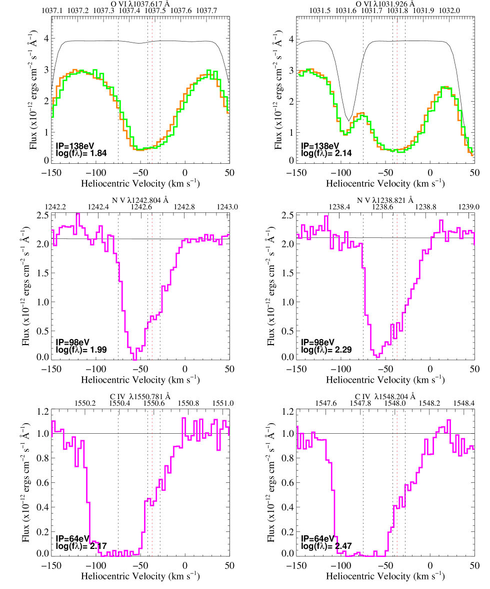
Figure 15.— Absorption as a function of velocity for the high ionization resonance lines of O VI, N V, and C IV, showing varying degrees of photospheric broadening to the red. Nebular outflow to the blue of systemic increases with decreasing ionization potential. See Figure 14 for a description of the colors.

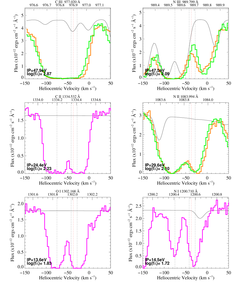
Figure 16.— Absorption as a function of velocity for representative C III, C II O I, N III, N II and N I lines. Ions are fully saturated throughout the nebular flow region blueward of –42 km s^-1. Neutrals are less so and favor strong absorption near –75 km s^-1. See Figure 14 for a description of the colors.

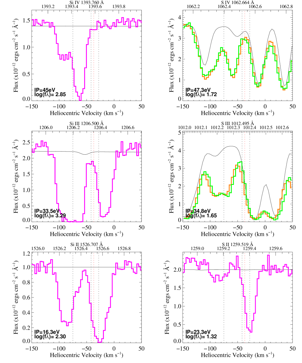
Figure 17.— Comparision of the Si IV – 2 to S IV – 2. The low ionization species, Si II and S II, dominate in the zone between –75 and –110 km s^-1 while the high ionization species, Si IV and S IV, dominate near –60 km s^-1. Transition in ionization occurs where absorption by the neutrals and H₂ is strongest. See Figure 14 for a description of the colors.

Comparison of the FUSE and STIS wavelength scales revealed a systematic offset. The reconciliation of this offset is essential for investigating the kinematics of the nebular outflow, where we seek to determine the velocity of the various molecular and atomic features with respect to the systemic velocity of the nebula. Lines that arise from the photosphere should match the systemic velocity of the system less the offset caused by gravitational redshift. An absolute reference to the heliocentric velocity was established by close examination of the O Ve $\lambda$1371.296 feature, shown in the middle panel of Figure 14. This narrow line results from a transition between two highly excited states in O Ve and is expected to be an excellent indicator of the photospheric restframe (Pierre Chayer private communication). For a compact object of this mass and radius (§ 2) we expect the photospheric lines to experience a gravitational redshift, $V_{gr}=c((1-\frac{2GM_{*}}{R_{*}c^{2}})^{-\text@frac{1}{2}}-1$) = 5.1 km s^-1. Applying a shift of –13 km s^-1 to the STIS spectrum placed the centroid of the O V $\lambda$1371.296 at –37 km s^-1, as expected for a $V_{sys}$ of –42 km s^-1 (Wilson, 1953).

Examination of overlapping FUSE and STIS spectra in the wavelength regions below 1190 Å revealed some systematic disagreements. In the original analysis of the FUSE M27 spectra by McCandliss (2001) the hot nebular H₂ component was defined to be at –69 km s^-1. We found it necessary to shift the FUSE spectra blueward by –6 km s^-1, such that the hot nebular H₂ is now at –75 km s^-1. The most useful overlap lines for assessing the alignment were the doublet blend of C IVe $\lambda\lambda$1168.849, 1168.993, bottom of Figure 14, and the the narrow O VIe $\lambda\lambda$1171.56, 1172.44, top of Figure 14. We note the wavelengths of O VIe doublet given in the National Institute of Standards and Technology (NIST) online tables (http://physics.nist.gov/PhysRefData/ASD/lines_form.html) appear to be in error by $\approx$ –0.42 Å (see Jahn et al., 2006). These spectra are comparatively noisy, but the alignment with the FUSE spectra agrees as well as the alignment between the s12 and s21 spectra. We also used the FUSE N I multiplets at $\lambda\lambda$1134 – 1135 and the STIS N I multiplets at $\lambda\lambda$1200 – 1201 along with excited H₂ lines that appear in the STIS bandpass above 1190 Å with the continuum plus hydrogen model of McCandliss & Kruk (2007) to assess the consistency of the wavelength reconciliation. The error in the systemic velocity (§ 2) is of order the FUSE resoution element and is three times the STIS resolution element. We consider the agreement of line profiles from spectra acquired with two different instruments to be excellent.

4.5.2 Photospheric + Nebular Features

O VI, N V and C IV

Figure 15 shows the high ionization resonance doublets of O VI $\lambda\lambda$1032.62, 1037.62, N V $\lambda\lambda$1238.821, 1242.804 and C IV $\lambda\lambda$1548.204, 1550.781. All these lines show photospheric absorption to the red of the systemic velocity. The strength and terminal velocity of the blue shifted portion of the line profiles increases with decreasing ionization potential. The O VI lines show only slight signs of blue shifted nebular absorption. The nebular absorption component in the N V lines is strong only between –42 and –75 km s^-1 just reaching saturation at $\approx$ –60 km s^-1. In contrast, the nebular absorption component in the C IV lines spans –42 to –115 km s^-1 and is completely saturated from –50 to –95 km s^-1.

4.5.3 Intermediate Ionic and Neutral Nebular Absorption

C III –  II, N III –  I and O I

Figure 16 show lines of C III –  II, N III –  I and O I. Like the C IV lines, the C III –  II lines are heavily saturated throughout the nebular flow region blueward of –42 km s^-1. The saturation makes it difficult to tell whether any one ion is dominant in the nebular outflow. N III is strongly blended with overlapping H₂ features. However, it shows saturated absorption between -60 and –100 km s^-1. N II $\lambda$1083.994 shows absorption throughout the flow, being less saturated at low velocities and becoming completely saturated at –75 km s^-1. This line also shows stronger nebular absorption than non-nebular absorption. In contrast, N I $\lambda$1200.223 shows weaker nebular absorption than non-nebular absorption. Both N I $\lambda$1200.223 and O I show an absorption component centered on –75 km s^-1, which coincides with the velocity of the absorption maximum in H₂ and C I.

Si IV –  II, and S IV –  II

The transition zone between high ionization and low ionization occurs at the velocity of –75 km s^-1 where H I, C I, N I, O I and H₂ show up most strongly in the nebula. The high ionization – low velocity, low ionization – high velocity dichotomy is best illustrated by examining the velocity profiles of the low abundance metals Si and S in Figure 17. Si II is stronger than Si IV in the zone between –75 and –110 km s^-1, while Si IV is stronger than Si II in the zone between –42 and –75 km s^-1. The Si III $\lambda$1206.500 line is saturated throughout most of the flow. The S IV – S II ions show similar behavior.

5. Discussion

Here we enumerate the main findings from the analysis.

1. The nebular H₂ is highly excited with a ground state ro-vibration population that deviates significantly from the best fit single temperature Boltzman distribution of 2040 K. The total column density is 7.9 $\times$ 10¹⁶ cm^-2. The deviations are characterized by a flatter slope for the lower rotational levels (0 $\leq\ J^{\prime\prime}\lesssim$ 5) than for the higher rotational levels (6 $\lesssim\ J^{\prime\prime}\leq$ 11).

2. Continuum fluorescence of H₂ has not been detected to the background limit of the sounding rocket observation $\approx$ 5 $\times$ 10^-17 ergs cm^-2 s^-1 Å^-1 arcsec^-2. However, Ly$\alpha$ fluorescence has been detected by Lupu et al. (2006). This emission mechanism is possible only for H₂ with a significant population in the $v\arcsec$ = 2 vibrational state in the presence of a strong Ly$\alpha$ radiation field.

3. The stellar SED exhibits negligible stellar reddening along the line-of-sight. This finding is at odds with the variable reddening indicated by the ratio of H$\alpha$/H$\beta$ intensity as reported in the literature and confirmed in this study in the immediate vicinity of the star. We note that the reddening determined by H$\gamma$/H$\beta$ and H$\delta$/H$\beta$ is consistent with zero and conclude it is possible that another physical process, aside from reddening by dust, is causing the discrepant H$\alpha$/H$\beta$.

4. The nebular H₂ appears at a heliocentric velocity of –75 km s^-1, corresponding to an expansion velocity of 33 km s^-1 in the nebular restframe. H I, C I, N I, and O I exhibit strong resonance line absorption at the same expansion velocity. The molecules and neutrals demarcate a transition velocity between a regime of high ionization and low expansion velocity (10 $\lesssim\ v_{hi}\lesssim$ 33 km s^-1) and a regime of low ionization and high velocity (33 $\lesssim\ v_{low}\lesssim$ 65 km s^-1). The upper limit to the terminal expansion velocity is $\approx$ 70 km s^-1. These observations, along with the absence of any signs for a high velocity radiation driven wind, are a challenge to interpret in the context of the simple interacting winds model for PN formation (Kwok et al., 1978). Meaburn (2005) (see also Meaburn et al., 2005a; Meaburn et al., 2005b), who used high resolution position-and-velocity spectroscopy of the optical emission lines to derive the ionization kinematics of several objects, have arrived at a similar conclusion. They find that ballistic ejection could have been more important than interacting winds in shaping the dynamics of PNe. Balick & Frank (2002) have reviewed in detail some of the more sophisticated thinking about the dynamical processes that shape PNe.

5. Analysis of the C I multiplet fine structure populations gives better agreement with the expected temperature of $\sim$ 2000 K for collisions with protons and electrons as opposed to collisions with neutrals or molecules. This suggests the molecular and neutral transition component is in close contact with ionized material.

6. The upper limits to CO in the diffuse line-of-sight gas range over 8 $\times$ 10¹³ cm^-2 $<N(CO)<$ 4 $\times$ 10¹⁴ cm^-2 depending on the assumed CO rotational excitation temperature. The high column density of C I found in the nebula is consistent with it being a daughter product of CO dissociation.

7. The lower limit to the neutral to H₂ column density ratio is $N$(H I)/$N(H_{2})$ = 127 in the transition region (using component number 3 in Table 2).

We will now discuss the constraints imposed by these findings on the ionization kinematics, mass structures, nebular dust, and the excitation, formation and destruction of H₂ within the nebula.

5.1. Ionization Kinematics

Low mass to intermediate mass stars begin to evolve into AGB stars when core nucleosynthesis ceases and a degenerate core forms. The AGB phase lasts $\approx$ 250,000 years and is marked by a series of high mass loss events that merge to produce a slow wind. At some point the star collapses into a hot compact degenerate object. In the PN formation scenario suggested by Kwok et al. (1978), a fast ($\sim$ 1000 km s^-1) low density radiation driven wind from the hot star shocks and ionizes the slow moving ($\sim$ 10 km s^-1), high density mostly molecular AGB wind, resulting in the expanding structures we see at latter times.

Natta & Hollenbach (1998) have computed detailed time dependent changes in the atomic and molecular emissions in a phenomenologically motivated interacting wind model. Their model consists of an interior ionization region bounded by a shell propagating outward with a velocity of 25 km s^-1 overrunning and shocking a mostly molecular AGB wind with a velocity of 8 km s^-1. An ionization-bounded time-dependent PDR results with three layers. These are, a fast moving ionized shock interface, an adjacent dissociation layer, and a slow moving molecular layer further downstream. They find most of the shell mass to be vibrationally excited H₂ and H I production to be modest. After $\approx$ 4000 years they find the infrared H₂ line diagnostic of S(1) (1–0) / S(1) (2–1) indicates a switch from thermal excitation to fluorescent excitation. They also find that H₂ does not co-exist with CO, as dissociation favors C⁺ + O. Consequently, they suggest molecular masses calculated for old PN based on CO emission and standard CO/H₂ ratios may be underestimated.

M27 has a kinematic age of $\approx$ 10,000 yrs (O’Dell et al., 2003), so perhaps it is reasonable that the nebula we see today bears little resemblance to this simple layered, two-velocity interacting wind picture. We see no evidence for a shell of predominately molecular material along the diffuse line-of-sight medium, nor do we see neutral or molecular material at low expansion velocity as would be expected for an unperturbed AGB wind. The upper limit to the molecular fraction in the neutral velocity component expanding at 33 km s^-1is $f_{H_{2}}$ = 0.016, assuming $N$(H)=$N$(H I). We do see evidence for velocity structure in the intermediate ionization states (Figures 16 – 17) and H I (Table 2) out to expansion velocities of $\approx$ 65 km s^-1, but there is no evidence for P-Cygni profiles with $\sim$ 1000 km s^-1 terminal velocities in any of the high ionization lines (Figure 15).

We find instead a rather permuted velocity structure of neutral and molecular material embedded (in velocity space) between the high and low ionization medium. Our findings suggest that the AGB wind has been accelerated through interaction with the hot star and that much of the original mostly molecular atmosphere has been almost completely dissociated. The surviving molecular material is currently interacting strongly with the highly ionized medium and we postulate that the intermediate ionization species are created and accelerated in this interaction.

Villaver et al. (2002b) have treated the radiative hydrodynamical problem with great rigor for a range of progenitor masses, using as a starting point for their PN simulation the structure found at end of AGB evolution by Villaver et al. (2002a). They find a main nebular shell develops surrounded by a relatively unperturbed halo. They give detailed figures for the evolution of density, velocity and H$\alpha$ emission brightness. We note that the amplitude of the velocity structures for their 1 – 2.5 M_sun models are in the range of the outflow velocities exhibited by the line profiles in Figures 15 – 17. Unfortunately they give no details on the ionization kinematics of the main and halo regions as a function of time, as Natta & Hollenbach (1998) have done. A model combining the detailed time dependent calculation of the atomic and molecular emissions of Natta & Hollenbach (1998) with the radiative hydrodynamical rigor of Villaver et al. (2002b) would be useful for interpreting these observations.

5.2. Mass Structures

Identifying kinematic components appearing in spectra with spatial structures in images must be approached with care. The computed total mass of these velocity components will depend on the assumed diameter and thickness of particular structures in the nebula. However, it seems reasonable to expect the 33 km s^-1 transition zone, where most of the molecular and much of the neutral hydrogen appears, to be at or near the region where the H$\alpha$ brightness drops to near zero. Inside this zone we expect the medium to be completely ionized. The minor axis of the bright H$\alpha$ in M27 is $\approx$ 300^′′ and the full diameter including the faint halo detected by Papamastorakis et al. (1993) is 1025″. Assuming a distance of 466 pc gives radii for the transition region and the total nebular extent to be $\approx$ 0.34 and 1.16 pc respectively. These radii agree reasonably well with the bright H$\alpha$ emitting region and the full extent of the AGB wind found in the Villaver et al. (2002a, b) simulations after $\approx$ 10,000 years .

We estimate the masses of the various structures given the following (gross) assumptions. Let the ionized region be a sphere with a radius of 0.34 pc and an electron density of $\sim$ 300 $\pm$ 200 cm^-3 (Barker, 1984). The ionized mass becomes 0.4 $\lesssim M_{ion}\lesssim$ 1.9 M_☉. If the total neutral hydrogen column density (3 $\times$ 10¹⁹ cm^-2) is uniformly distributed in a shell between 0.34 and 1.16 pc with a mean density of 12 cm^-3, then $M_{sh}$ = 1.7 M_☉. Our constraint on the progenitor mass, the sum of the ionized, shell and degenerate star masses, is 2.6 $\lesssim M_{pro}\lesssim$ 4.2 M_☉.

By comparison, the molecular material in the diffuse nebular medium has a much lower mass. Although the H₂ is associated with only one neutral hydrogen velocity component, we assume it is spread uniformly throughout the 0.82 pc thick shell. Using this maximal volume yields an upper limit on the molecular mass in the diffuse medium, $M_{dmol}\lesssim$ (1.7 M_☉)/375 = 4 $\times$ 10^-3 M_☉. Meaburn & Lopez (1993) have estimated the total mass of the eleven largest globules, which appear as dark knots against the bright nebular O III emission, to be $M_{omol}$ = 1.1 $\times$ 10^-3 M_☉. They used measurements of O III transmission and assumed the general ISM gas-to-dust ratio (Bohlin et al., 1978). The Meaburn et al. clump mass estimates compare reasonably well to those of Huggins et al. (1996) who estimate the total molecular mass associated with the CO emitting clumps to be $M_{cmol}$ = 2.5 $\times$ 10^-3 M_☉. They assumed a thin ring geometry and a fraction of CO/H₂ = 3 $\times$ 10^-4, a value $\geq$ 10 times than the highest found by Burgh et al. (2007) for the diffuse ISM. Use of a lower ratio will increase the CO clump mass estimate as noted by Natta & Hollenbach (1998).

Our upper limit to the diffuse molecular mass is on the same order as the clump mass estimates. The upper limit on the total molecular mass in the nebula, the sum of the diffuse and CO derived masses (assuming the high CO/H₂ ratio), is M_mol = 6.5 $\times$ 10^-3 M_☉. We conclude that there is no large mass of molecular material in M27, either in the diffuse or clumped medium. This is in contrast to the Meixner et al. (2005) finding for the Helix, for which they estimate the mass of all the H₂ emitting globules to be $\sim$ 0.35 M_☉. We note that all of the molecular mass estimates for M27 are on the order of the mass of the planets in our own solar system, $\approx$ 1.3 $\times$ 10^-3 M_☉. The suggestion that dense circumstellar bodies have survived the AGB phase and may constitute a significant fraction of the molecular material in the nebula environment cannot be ruled out.

The absence of CO absorption in the diffuse medium is consistent with the Natta & Hollenbach (1998) finding that CO and H₂ are unlikely to co-exist in the gas phase, because CO is quickly dissociated after leaving the vicinity of the clumps. Huggins et al. (2002) confirmed this picture with exquisite observations of the globules of the Helix. They show how CO survives only in the shadows of the clumps. The heads of these globules show strong coincident emission of H₂ S(1) (1–0) and H$\alpha$, and weaker coincident emission in the shadowed zone. O’Dell et al. (2003) note the globules in M27 tend towards a more irregular and tail-less appearence than those in the Helix. Nevertheless the observation of H₂ emission in the vicinity of the globules suggests they may be a source of H₂ for the diffuse nebular medium.

The temperature of the diffuse medium inferred from the molecular hydgrogen ro-vibration levels exceeds the sublimation temperature of refractory dust, $\sim$ 1500 K (Glassgold, 1996). While it is unlikely that the gas and dust will be in thermodynamic equilibrium, the absence of any significant reddening of the central star SED suggests that the diffuse environment is as inhospitable to dust as it is to CO and H₂. Dust, or perhaps even compact bodies, may exist in the CO rich dense clumps, which we will argue in § 5.3.2, are the likely source of H₂ for the diffuse medium.

5.3. Constraints on the Excitation, Formation and Destruction of H₂

5.3.1 H₂ Excitation Processes

The models of Natta & Hollenbach (1998) suggest that in the latter stages of planetary nebula evolution the H₂ is being excited via far-UV continuum fluorescence, yet we have failed to detect this emission. We briefly review this process.

H₂ is excited from the ground vibrational level of $X\,^{1}\Sigma_{g}^{+}$ into higher electronic states, predominately $B\,^{1}\Sigma_{u}^{+}$  and $C\,^{1}\Pi_{u}$ (the Lyman and Werner bands), by the absorption of a far-UV photon (912 $\leq$ $\lambda$ $\lesssim$ 1120 Å) emitted by a star. The short wavelength cutoff is imposed by the usual assumption that enough neutral hydrogen is present to shield H₂ from excitation by stellar Lyman continuum (Lyc) photons. The rate of molecular excitation is proportional to the stellar flux absorbed by the ro-vibrational population of the ground electronic state $X\,^{1}\Sigma_{g}^{+}$. Fluorescence follows excitation, producing a highly structured emission in the 912 – 1650 Å bandpass, as electrons fall back into the excited vibrational levels of $X\,^{1}\Sigma_{g}^{+}$. Approximately 11 - 15$\%$ of the time, the fluorescent pumping process leaves the molecule in the vibrational continuum of the ground state ($X\,^{1}\Sigma_{g}^{+}$), located 4.48 eV above the ($J\arcsec$,$v\arcsec$) = (0,0) level, resulting in its spontaneous dissociation into $H(1s)+H(1s)$ (Stecher & Williams, 1967; Dalgarno & Stephens, 1970; Draine & Bertoldi, 1996). Electrons ending up below the vibrational continuum cascade toward the ground vibrational state $v\arcsec$ = 0 via slow quadrupole transitions with radiative lifetimes $\sim$ few days and longer (Wolniewicz et al., 1998), producing the infrared fluorescence spectrum (Black & Dalgarno, 1976).

Lyman and Werner band absorption of the central star continuum unavoidably results in ultraviolet fluorescence, so why was it not detected? To answer this question we estimate the total brightness by simply calculating how many stellar photons are absorbed by H₂ at a given distance, which we take to be the transition zone, and re-emitted into 4$\pi$ steradians. This will give an upper limit to the total brightness of the H₂ in the diffuse medium. We will neglect absorption by dust.

Using our hydrogen absorption model we find 30% of the photon flux in the 912 – 1120 Å bandpass is absorbed. Reradiation into 4$\pi$ steradians at 0.34 pc yields a total brightness of 3.4 $\times$ 10^-5 ergs cm^-2 s^-1 sr^-1(assuming an average energy per photon of 1.6 $\times$ 10^-11 ergs). Neglecting the fluorescence redistribution into specific lines, and averaging over a 910 – 1660 Å bandpass, we find an upper limit to the mean brightness of the continuum fluorescence of 1.1 $\times$ 10^-18 ergs cm^-2 s^-1 Å^-1 arcsec^-2. This is a factor of $\sim$ 50 below the background estimate shown in Figure 3. So we find the continuum fluorescence is not very bright and shows no sign of contributing to the ground state ro-vibrational population, as there is little in the way of absorption arising from vibrational levels $v\arcsec$ $>$ 2. This is in contrast to the strong indication of continuum fluorescence found in the reflection nebula NGC 2023 by Meyer et al. (2001), where they observed absorption lines from all $v\arcsec$ $\leq$ 14 states of $X\,^{1}\Sigma_{g}^{+}$ in a STIS spectrum of the central star HD 37903.

The low levels of continuum fluorescence found here are consistent with the infrared spectroscopic diagnostics presented by Zuckerman & Gatley (1988), who found the ratio of S(1) (1–0) / S(1) (2–1) (at 2.122 and 2.248 $\mu$m respectively) to be $\approx$ 10, placing it in the thermal regime well above the value of 2 expected from fluorescence (Black & Dalgarno, 1976). If the S(1) (1–0) line were produced by fluorescence, then the 10^-4 ergs cm^-2 s^-1 sr^-1 measured by Zuckerman & Gatley (1988) would imply a total ultraviolet brightness $\sim$ 850 times this value (in energy units, 50 times in photon units) and would have easily been detected by the rocket experiment.

The detection of Ly$\alpha$  fluorescence pumped through two resonant transitions in the $v\arcsec$= 2 vibrational level of the $X\,^{1}\Sigma_{g}^{+}$ electronic state (R(6) (1–2) at 1215.730 Å and P(5)(1–2) at 1216.073) reported recently by Lupu et al. (2006), serves to emphasize that in a radiation bounded nebula two-thirds of the Lyc photons emitted by the star are converted to Ly$\alpha$ photons (Spitzer, 1998). The contrast between the Ly$\alpha$ and continuum fluorescence is enhanced in our case, because the number of Lyc photons exceeds the number of photons in the 912 – 1120 Å bandpass by a factor of 15. Even so, modeling by Lupu et al. (2006) shows the Ly$\alpha$ fluorescence rate is too low to cause detectable deviations in a thermalized groundstate population at a temperature of 2000 K. We conclude that the observed ro-vibration population distribution of the hot H₂ is dominated by collisional processes. The deviations from a pure thermal distribution will be addressed in § 5.4.

5.3.2 Molecular Hydrogen Formation and Destruction

The observed neutral atomic to molecular hydrogen ratio ($\frac{N(HI)}{N(H_{2})}$ = 127) can be used to constrain formation and destruction processes in the diffuse nebular medium using the formula,

$$\frac{dn_{2}}{dt}=F-Dn_{2}.$$ (2)

$F$is the sum over all formation processes, $D$ is the sum over all destruction processes, and $n_{2}$ is the density of H₂. We will not attempt to provide a comprehensive listing of all the processes, rather we will make some limiting assumptions to develop the constraints.

In the limit where formation is absent ($F$ = 0) the solution for $n_{2}(t)$ is an exponential with an e-fold time equal to $D^{-1}$. If we assume the destruction process is radiative dissociation, then $D=\chi p_{diss}\zeta_{pump}$, where $p_{diss}$ is the mean dissociation fraction, $\zeta_{pump}$ is the mean probability per second of an upward radiative transition and $\chi$ the standard interstellar radiation field multiplier. Draine & Bertoldi (1996) have conveniently tabulated $\zeta_{pump}$ and $p_{diss}$ for a number of transitions for $\chi$ = 1, neglecting self-shielding. They find fairly narrow ranges for $\zeta_{pump}$ and $p_{diss}$ and weighted mean values of these products over the H₂ ground state ro-vibrational distribution are relatively insensitive to the actual distribution for our purposes here. We will use $p_{diss}$ = 0.15 and $\zeta_{pump}$ = 3.5 $\times$ 10^-10 s^-1, yielding $D_{1}$ = 5.3 $\times$ 10^-11 s^-1 as a representative dissociation rate for $\chi$ = 1.

To compute $\chi$ we use the Rauch model, which has a total photon luminosity of 1.2 $\times$ 10⁴⁵ ph s^-1 in the 912 – 1120 Å bandpass at the stellar surface. At 0.34 pc, the photon flux is 8.9 $\times$ 10⁷ ph cm^-2 s^-1, yielding a rather modest scale factor of $\chi$ = 7.4 relative to the average ISM background of 1.2 $\times$ 10⁷ ph cm^-2 s^-1 (Draine & Bertoldi, 1996). The resulting e-fold time for radiative dissociation is 21 years and it would only take 100 years for the $\frac{N(HI)}{N(H_{2})}$ ratio to reach its currently observed level. We conclude the source term for the diffuse medium $F\neq$ 0, i.e. the H₂ in the diffuse medium must be constantly replenished.

We now turn to the equilibrium limit, i.e. $\frac{dn_{2}}{dt}=0$. The formation term is $F=\gamma nn_{1}$ where the neutral hydrogen density is $n_{1}$. We consider either formation of H₂ by dust, or by associative detachment $H+H^{-}\rightarrow H_{2}+e^{-}$. In the former case $\gamma_{d}$ = 3 $\times$ 10^-17 cm³ s^-1 (Natta & Hollenbach, 1998) and $n$ is the gas density. In the latter case $n$ is the electron density $n_{e}$ and $\gamma_{-}$ is given by Eq. 15 of Natta & Hollenbach (1998). The rate coefficient ($\gamma_{-}$) depends explictly on hydrogen ionization fraction and temperature. At $T$ = 2000 K we find $\gamma_{-}$ $\approx$ $\gamma_{d}$ when the ionization fraction $x_{+}\equiv$ $n_{+}/(n_{1}+n_{+})$ = 0.5. When $x_{+}$ = 0.05, $\gamma_{-}$ $\approx$ 15$\gamma_{d}$.

Equating formation and destruction we solve for the total density $n$ required for formation to keep pace with dissociation. With $\chi$ = 7.4 the dissociation rate is $D$ = 3.9 $\times$ 10^-10 s^-1 and we find, $n=\frac{D}{\gamma}\frac{n_{2}}{n_{1}}$ = 10⁵ cm^-3 for the dust and the $x_{+}$ = 0.5 cases. For $x_{+}$ = 0.05 the density is $\approx$ 7000 cm^-3. These densities are consistent with the Meaburn & Lopez (1993) clump estimates for M27, but they are much higher than the gas and electron densities we found from the C I analysis in § 4.4.2 for the transition zone or the electron density given by Barker (1984) for the ionized region.

We conclude that the density in the diffuse medium is not high enough to support formation of H₂ either on dust grains or through the associative detachment processes and that the most likely source of excited H₂ is from photo-evaporating clumps (c.f. Huggins et al., 2002; López-Martín et al., 2001). Whether the clumps are reservoirs of H₂ that formed long ago or are currently active in forming H₂ by these processes is an open question. The transport process that moves molecular hydrogen out of the clumpy medium and constantly replenishes the diffuse medium is a dynamical process, which results in the exposure of H₂ to Lyc radiation.

Figure 18.— Energy level diagram illustrating the threshold energy ro-vibration levels ($J\arcsec$,$v\arcsec$) that can be excited to Rydberg orbitals ($H(1s)+H(nl),2\leq n\leq\infty,l=s,p,d...$) with photons energies $\leq$ 13.6 eV. The threshold for excitation into the H${}_{2}^{+}$ cation ground state is also shown. Normalized Maxwell-Boltzmann energy distributions for $T$ = 10000, 4000 and 2000 K show schematically the relative change in the energy level population as a function of temperature.

5.4. Beyond Spontaneous Dissociation – Lyc Dissociation and Photoionization of H₂

We have two outstanding puzzles. One is the apparent “two temperature” slope in the ro-vibration population (Figure 9). The other is the excess H$\alpha$/H$\beta$ ratio in the absence of any significant stellar or nebular reddening. We speculate here that a confluence of environmental factors – molecular hydrogen interacting and excited by a ionized medium that is optically thin to Lyc radiation – conspire to contribute to the production of H$\alpha$ emission at a few percent of the radiative recombination rate and to create the two temperature slope.

We know that while the energies of thermal electrons in the nebula are high enough to populate the $X\,^{1}\Sigma_{g}^{+}$ vibrational levels above $v\arcsec$ $>$ 0, they are not nearly high enough to lead to dissociative excitation. For that a radiative process is required such that $H_{2}(X\,^{1}\Sigma_{g}^{+})+\gamma$ ultimately results in $H(1s)+H(3p)$, which can then branch into Ly$\beta$ or H$\alpha$ + Ly$\alpha$. Stecher & Williams (1967) discussed two possible radiative paths that lead to the dissociation of H₂. In § 5.3.1 we described the familiar spontaneous dissociation process that leads to $H(1s)+H(1s)$ following excitation into the Lyman ($B\,^{1}\Sigma_{u}^{+}$) and Werner ($C\,^{1}\Pi_{u}$) bands. The other path (with multiple channels) is,

$$H_{2}(X\,^{1}\Sigma_{g}^{+})+\gamma\rightarrow\left\{\begin{array}[]{ll}H(1s)+H(nl)&Pre-and~{}direct-dissociation,\\ H_{2}^{+}(X\,^{2}\Sigma_{g}^{+})+e^{-}&Photoionization,\end{array}\right.$$ (3)

with $n\geq$2 and l = s, p, d … the angular momentum of the excited atom. The photoionization channel can further undergo dissociative recombination with low energy electrons,

$$H_{2}^{+}(X\,^{2}\Sigma_{g}^{+})+e^{-}\rightarrow H(1s)+H(nl).$$ (4)

These channels are not usually considered to be important for H I regions (PDRs) because the photoionization, pre-dissociation and direct-dissociation processes all have thresholds above the Lyman limit. In such an instance the H₂ is usually cold and optically thick neutral hydrogen shields the H₂ from dissociation (Spitzer, 1948). However for H₂ in H II regions it is not at all clear that this assumption is justified. At the interface of a mostly molecular clump embedded in an ionized medium, as we encounter in M27, there will be a zone where the H I and H₂ are optically thin to ionizing radiation and the H₂ is excited (hot). In this case the ionization and dissociation of H₂ by photons with energies above the Lyman limit at 13.598 eV should also be considered.

Direct-dissociation paths proceed through excited ro-vibrational levels in the $B\,^{1}\Sigma_{u}^{+}$, $B^{\prime}\,{}^{1}\Sigma_{u}^{+}$ and $C\,^{1}\Pi_{u}$ upper electronic states of H₂, while the $B^{\prime\prime}\,{}^{1}\Sigma_{u}^{+}$, $D\,^{1}\Pi_{u}$, $D^{\prime}\,{}^{1}\Pi_{u}$ and $D^{\prime\prime}\,{}^{1}\Pi_{u}$ states can under go pre-dissociation as well as direct-dissociation. The experimental distinction is that a pre-dissociation process shows structure (in the absorption cross-sections as a function of wavelength) while direct-dissociation does not (Lee & Judge, 1976). The structure is a consequence of the perturbative coupling with the dissociative continuum of the overlapping excited electronic states.

The vibrational continua of the upper electronic states converge into Rydberg orbitals, which are essentially n $\geq$ 2 principal quantum number electrons in orbital around the cation (H${}_{2}^{+}$) core. At asymptotic nuclear separation these orbitals become free $H(1s)+H(nl)$. Transitions between $X\,^{1}\Sigma_{g}^{+}$ and its own vibrational continuum ($H(1s)+H(1s)$) at 4.48 eV can proceed only by quadrupole radiation, while transitions between $X\,^{1}\Sigma_{g}^{+}$ and the upper singlet electronic states are dipole allowed. The vibrational continua of $B\,^{1}\Sigma_{u}^{+}$, $B^{\prime}\,{}^{1}\Sigma_{u}^{+}$, and $C\,^{1}\Pi_{u}$ converge to $H(1s)+H(2l)$ at 14.67 eV (844.8 Å), $D\,^{1}\Pi_{u}$ and $B^{\prime\prime}\,{}^{1}\Sigma_{u}^{+}$ converge to $H(1s)+H(3l)$ at 16.56 eV (748.46 Å), $D^{\prime}\,{}^{1}\Pi_{u}$ converges to $H(1s)+H(4l)$ at 17.22 eV (719.74 Å) and $D^{\prime\prime}\,{}^{1}\Pi_{u}$ converges to $H(1s)+H(5l)$ at 17.52 eV (707.175 Å), measured with respect to ($J\arcsec$, $v\arcsec$) = (0,0) of H₂ $X\,^{1}\Sigma_{g}^{+}$. The onset of photoionization (H₂ + $\gamma$ $\rightarrow$ H${}_{2}^{+}$ + e^-) is at 15.43 eV (803.7 Å) in between the $H(1s)+H(2l)$ and $H(1s)+H(3l)$. The right side of Figure 18 shows the energy levels of Rydberg states in relation to the cation ground state.

Glass-Maujean et al. (1986) give cross sections for the photo-excitation of Ly$\alpha$ ($H(1s)+H(2l)$) from the direct- and pre-dissociation of H₂($X\,^{1}\Sigma_{g}^{+}$). The total cross section peaks at the threshold (14.67 eV), reaching 5 $\times$ 10^-18 cm² and falls monotonically thereafter. Cook & Metzger (1964) have shown the detailed structure in the H₂ photo-dissociation and ionization cross section from 550 – 1000 Å. The photoionization cross section peaks near 18 eV at $\approx$ 10^-17 cm². Some of the discrete dissociation peaks to the red are $\approx$ a factor of 3 higher at a resolution limit of 0.5 Å. Flannery et al. (1977) have calculated and tabulated cross sections for excitation out of vibrationally excited states of H₂($X\,^{1}\Sigma_{g}^{+}$,$v\arcsec$) + $\gamma\rightarrow$ H${}_{2}^{+}$($X\,^{2}\Sigma_{g}^{+}$, $v^{\prime}$) + $e^{-}$ as a function of wavelength, assuming $\Delta J$ = 0.

Yan et al. (1998) produced a piecewise continuous function for the photoionization cross section valid over the interval 300 $\geq E_{ph}\geq$ 15.4 eV. At high frequencies the cross section for H₂ ionization is 2.8 times that for H I. Above 18.09 eV H₂ can undergo dissociative ionization, H₂ + $\gamma$ $\rightarrow$ H + H⁺ + e^-, or even H⁺ + H⁺ + 2e^-, but the branching ratios into these channels are small over the wavelengths of Lyc emitted by the central star (see Yan et al., 1998, and references therein) where the yield for dissociative recombination should be $p_{dr}$ $\approx$ 1.

Stecher & Williams (1967) have noted how the thresholds for transition into the upper level continua are lower for excited ro-vibrational ($J\arcsec$, $v\arcsec$) levels of $X\,^{1}\Sigma_{g}^{+}$. Cook & Metzger (1964) observed this effect in the redward broadening of the dissociation thresholds by $\approx$ 14 Å in their experiments conducted at room temperature. It is actually possible to dissociate and photoionize H₂ with photon energies less than the Lyman limit, for a high enough ro-vibrational level ($J\arcsec$, $v\arcsec$). We quantify this in Figure 18 where the energies of the ro-vibrational levels in the $X\,^{1}\Sigma_{g}^{+}$ state in relation to the asymptotically free states are shown. Horizontal lines drawn through the ($v\arcsec$, $J\arcsec$) energy levels indicate the thresholds for excitation with photons $\leq$ 13.6 eV in energy. Maxwell-Boltzmann Energy distributions with temperatures of 2000, 4000 and 10000 K are drawn to indicate schematically how the relative populations of the upper levels change as a function of $T$.

Rotational states above $J\arcsec$ = 13 in $v\arcsec$ = 0, $J\arcsec$ = 9 in $v\arcsec$ = 1, and $J\arcsec$ = 3 in $v\arcsec$ = 2 can be excited to $H(1s)+H(2p)$ by photons with energies $\leq$ 13.6 eV. The steepening of the slope of the level population in Figure 9 might result from a radiative depopulation of the higher J” states into the asymptotic $H(1s)+H(2p)$ state. The populations of the upper levels become selectively depleted, a process we refer to as “radiative skimming.” However, the slope change in the $v\arcsec$ = 0, 1 curves are observed to occur at at $J\arcsec$ $\approx$ 6, 8 respectively, which are smaller than given above. We take this as evidence for skimming by Lyc photons.

We also see from Figure 18 that the creation of $H(1s)+H(3p)$ without the benefit of Lyc photons would require extremely high temperatures $\gtrsim$ 4000 K. The two step process H₂($X\,^{1}\Sigma_{g}^{+}$) + $\gamma\rightarrow$ H${}_{2}^{+}$($X\,^{2}\Sigma_{g}^{+}$) + $e^{-}\rightarrow H(1s)+H(3p)$ is energetically more accessible than the direct $H_{2}(X\,^{1}\Sigma_{g}^{+})+\gamma\rightarrow H(1s)+H(3p)$. Observations by Lee & Judge (1976) of the direct production of Balmer series fluorescence from H₂ by direct- and pre-dissociation support this conjecture. They find the dissociation yield with respect to total dissociation + photoionization cross section to be on the order of a few percent. For example, at 716 Å the cross section for production of H$\alpha$  was 0.23 $\times$ 10^-18 cm ², which is about a factor of 40 lower than for the production of H${}_{2}^{+}$.

H${}_{2}^{+}$ is also homonuclear (Leach & Moss, 1995), so radiative transitions among the 18 vibrational levels of the $X\,^{2}\Sigma_{g}^{+}$ ground state are not dipole allowed. The vibrational continuum of H${}_{2}^{+}$ $X\,^{2}\Sigma_{g}^{+}$  ($H^{+}+H(1s)$) is only 2.646 eV above the ($J\arcsec$, $v\arcsec$) = (0,0) ground state, so electron energy need not be high to produce dissociative recombination into the overlapping Rydberg states. Excitation to higher bound states, (${}^{2}\Sigma^{+}_{g}$, ${}^{2}\Pi_{u}$) have poor overlap integrals (Franck-Condon factors) yielding small branching ratios to these dipole allowed upper levels. Once created, H${}_{2}^{+}$ will undergo rapid dissociative recombination with free electrons, H${}_{2}^{+}$ + $e^{-}\rightarrow H(1s)+H(nl)$, producing a fluorescent cascade of Lyman and Balmer emission. The amount of H$\alpha$ and Ly$\alpha$ produced will depend upon the vibrational distribution in the cation energy levels and the electron impact energies.

Takagi (2002) has shown in detail how the dissociative recombination cross sections of the individual $H(nl)$ channels depends strongly on the vibrational level of the H${}_{2}^{+}$ $X\,^{2}\Sigma_{g}^{+}$($v\arcsec$) state. The cross sections are generally highest for e^- collisions with the lowest energies and fall in proportion to the inverse of the electron energy. Typical values near zero electron energy range from 10^-15 – 10^-17 cm² ignoring rotation. Including the rotational state introduces resonances and can strongly modulate the cross sections at low electron energies. Schneider et al. (1994) have calculated total dissociative recombination rates for H${}_{2}^{+}$ for hydrogen plasmas with temperatures between 20 – 4000 K for individual ro-vibrational states of H${}_{2}^{+}$, but they provide no estimate of the branching ratios into the individual $H(1s)+H(nl)$ final states.

5.5. Optically Thin Photoionization Destruction of H₂ 

We have suggested that photoionization by Lyc photons of excited H₂ in an optically thin medium ultimately results in a fluorescent cascade of Lyman and Balmer emission. Verification of this hypothesis will require exploring the detailed balance of hydrogen ions, atoms and molecules in the recombination regime between Case A (the optically thin limit where Lyman series emissions are not reabsorbed in the nebula) and Case B (the optically thick limit where Lyman series emissions are reabsorbed on the spot).

In the previous section we have given references to the necessary molecular cross sections for computing the photoionization rates out of the vibrationally excited molecule and into the excited cation (Flannery et al., 1977), along with the cross sections for electron impact dissociation of excited cation states into the Rydberg manifold (Takagi, 2002). The calculation of the Lyman and Balmer series emissivity resulting from the two step process of molecular photoionization followed by dissociative recombination goes beyond the scope of this paper.

Here we show an example of the competitiveness of photoionization with spontaneous dissociation for the destruction of H₂ in the optically thin limit. The ionization rates at the transition zone (0.34 pc) for H₂ and H I were calculated by integrating the cross sections for these species, using Yan et al. (1998) for H₂ and Spitzer (1998, Eq. 5-4) for H I, over the SED of our stellar model from $\lambda<$ 911.7 Å according to Spitzer (Eq. 4-36, 1998). We do not include contributions from direct and pre-dissociation processes, which are likely to be substantial for excited H₂, so our dissociation estimate will be conservative. We find $\zeta_{H2\rightarrow H2+}$ = 3.4 $\times$ 10^-9 s^-1 compared to $\zeta_{H\rightarrow H+}$ = 1.4 $\times$ 10^-9 s^-1. The ratio is 2.4, so we conclude that in the optically thin limit it is easier to ionize the hydrogen molecule than the atom.

In an optically thin medium at the inferred radius of the transition zone the molecular photoionization rate $\zeta_{H2\rightarrow H2+}$ exceeds the far-UV pump rate $\chi\zeta_{pump}$ (§ 5.3.2) by a factor of 1.3. If we assume that the yield for dissociative recombination (H${}_{2}^{+}$ + e^- $\rightarrow H(1s)+H(nl)$) following creation of the cation is 100%, then the photoionization mediated dissociation of H₂ can be expected to be $p_{dr}\zeta_{H2\rightarrow H2+}$ / ($p_{diss}\chi\zeta_{pump})\approx$ 9 times the spontaneous dissociation. This process increases the rate required for the clumps to resupply the diffuse medium with H₂ in the steady state limit. We note that Natta & Hollenbach (1998) do not include Lyc dissociation of H₂ in their model. This may be why they find the shell mass is dominated by H₂ as opposed our finding that $\frac{N(HI)}{N(H_{2})}\gg$ 1.

6. Conclusions and Suggestions for Future Investigations

M27 is an excellent laboratory for testing theories of formation, excitation and destruction of molecules and dust, because the stellar temperature, mass, gravity, as well as the nebular distance, masses, abundances and excitation states, are well quantified.

We find that the diffuse nebular medium is generally inhospitable to molecules and dust. The diffuse H₂ accounts for a small fraction ($\sim$ 0.3 %) of the total nebular mass. H₂ is easily destroyed by the stellar radiation field in the diffuse medium on a timescale $\sim$ 20 years. A steady state abundance requires a source, most likely the clumpy medium. If the clump density is high enough, they may support molecular hydrogen formation via dust or mediated by radiative detachment, although we cannot rule out photoevaporation of relic material.

The finding of neutrals and molecules at a transition velocity between slow-high and fast-low ionization material suggests collisional interaction with charged particles is the most important process for establishing the observed ro-vibration level populations in molecular hydrogen. Lupu et al. (2006) finds the rate of Ly$\alpha$ pumping is not high enough to change the level population of a thermal distribution and we find the rate of continuum pumped fluorescence is even lower. However, if the neutral hydrogen is optically thin in the transition zone, then stellar Lyc can radiatively skim the upper rotational states of $v\arcsec$ = 0, 1 and create the apparent break in the high and low temperature slopes at the observed levels, but this is likely to be a second order process.

Dissociation and ionization of the hydrogen molecule by Lyc photons can also lead to the production of Lyman and Balmer series emission and may provide an explanation for the excess H$\alpha$/H$\beta$ ratio observed in the apparent absence of extinction by dust. In the optically thin limit Lyc mediated destruction rates can exceed by an order of magnitude the spontaneous dissociation rate and should be considered when calculating the equilibrium abundance of excited H₂ in H II regions.

At this late stage in the evolution of M27 most of the original AGB atmosphere has been dissociated and accelerated to velocities in excess of 33 km s^-1 but not above 68 km s^-1. A high speed radiation driven stellar wind is not detected in the present epoch. The mechanism for acceleration remains unidentified.

The analysis of the formation and destruction of H₂ rests in part on the determination of the H I velocity structures identified in the Dwingeloo survey data to guide the column density determination carried out with the STIS and FUSE data. However, our conclusions regarding the overall abundance of molecular hydrogen with respect to H I and the need for a molecular source for the diffuse medium are immune to changes in the atomic abundance by factors of 10. Nevertheless it would be prudent to check the velocity structure found here with a high resolution mapping using a telescope with a smaller beam ($\approx$ 4′). It appears that the velocity separation of M27 permits discrimination with respect to the galactic H I background. This and a reasonable signal strength have allowed the apparent detection of H I in a PN where only upper limits have existed previously (Schneider et al., 1987).

Our lowest bound for $N(CO)/N(H_{2})$ $<$ 10^-3 in the diffuse nebular medium, is a factor of 30 higher than ratio used by Huggins et al. (1996) to constrain the CO clump mass. Should a HST servicing mission 4 be successful in resurrecting STIS then higher signal-to-noise data could be acquired to examine the $N(CO)/N(H_{2})$ more carefully, using a number of rovibrational bands. It should be possible to place limits on $\log{N(CO)}\lesssim$ 13 (e.g. Burgh et al., 2007).

We emphasize that our analysis applies to the direct line of sight gas, the diffuse nebular medium, which we find to be dust free. The existence of clumps with column densities of CO in excess of 10¹⁶ cm^-2 immediately adjacent to regions with CO column densities $\lesssim$ 10¹⁴ cm^-2 attests to the steep density gradients within the nebular environment and the probable low covering fraction of the densest clumpy medium. The clumps may well be reservoirs of material depleted from the diffuse medium. Measuring the abundance of metals on either side of the neutral transition velocity could provide information on whether photo-evaporation of the globules is an important process for the enrichment of metals in the high velocity zone (McCandliss & Kruk, 2007). In addition, infrared spectral and imaging observations with Spitzer could tell us much more about the prevalence of dust and molecules elsewhere in the nebula. Mapping of the nebular Balmer emission line ratios with respect to the H₂ S(1) (2–1) / S(1) (1–0) emission ratio would be especially useful for further exploring the connections between H₂ production of Balmer emission and the prevelence of thermal or fluorescence processes in the clumpy medium.

During the review of this paper, work by O’Dell et al. (2007) was brought to our attention. O’Dell et al. derive the total flux in the infrared H₂ emission lines in the Helix Nebula and argue that only Lyc radiation from the star has enough power to sustain the H₂ IR emission at the observed levels. They also propose that charge exchange between H₂ and O⁺ could be a significant dissociation channel. Future work examining the efficiency of their proposed charge exchange mechanism for mediating the dissociation of H₂ in comparison to the Lyc dissociation process proposed here, would be a useful addition to the nascent field of Lyc dominated PDR’s.

References

- Abgrall et al. (1993a) Abgrall, H., Roueff, E., Launay, F., Roncin, J. Y., & Subtil, J. L. 1993a, A&AS, 101, 273
- Abgrall et al. (1993b) Abgrall, H., Roueff, E., Launay, F., Roncin, J. Y., & Subtil, J. L. 1993b, A&AS, 101, 323
- Aleman & Gruenwald (2004) Aleman, I., & Gruenwald, R. 2004, ApJ, 607, 865
- Bachiller et al. (2000) Bachiller, R., Cox, P., Josselin, E., Huggins, P. J., Forveille, T., Miville-Deschênes, M. A., & Boulanger, F. 2000, in ESA SP-456: ISO Beyond the Peaks: The 2nd ISO Workshop on Analytical Spectroscopy, 171
- Balick & Frank (2002) Balick, B., & Frank, A. 2002, ARA&A, 40, 439
- Barker (1984) Barker, T. 1984, ApJ, 284, 589
- Benedict et al. (2003) Benedict, G. F., et al. 2003, AJ, 126, 2549
- Black & Dalgarno (1976) Black, J. H., & Dalgarno, A. 1976, ApJ, 203, 132
- Bohlin et al. (2001) Bohlin, R. C., Dickinson, M. E., & Calzetti, D. 2001, AJ, 122, 2118
- Bohlin et al. (1978) Bohlin, R. C., Savage, B. D., & Drake, J. F. 1978, ApJ, 224, 132
- Brocklehurst (1971) Brocklehurst, M. 1971, MNRAS, 153, 471
- Burgh et al. (2007) Burgh, E. B., France, K., & McCandliss, S. R. 2007, submitted to ApJ
- Burgh et al. (2002) Burgh, E. B., McCandliss, S. R., & Feldman, P. D. 2002, ApJ, 575, 240
- Burgh et al. (2001) Burgh, E. B., McCandliss, S. R., Pelton, R., France, K., & Feldman, P. D. 2001, in Proc. SPIE Vol. 4498, p. 296-302, UV/EUV and Visible Space Instrumentation for Astronomy and Solar Physics, Oswald H. Siegmund; Silvano Fineschi; Mark A. Gummin; Eds., 296
- Burnham (1978) Burnham, R. 1978, Burnham’s celestial handbook. an observers guide to the universe beyond the solar system (New York: Dover, 1978, Rev.ed.)
- Cahn (1976) Cahn, J. H. 1976, AJ, 81, 407
- Cahn et al. (1992) Cahn, J. H., Kaler, J. B., & Stanghellini, L. 1992, A&AS, 94, 399
- Capriotti (1973) Capriotti, E. R. 1973, ApJ, 179, 495
- Cardelli et al. (1989) Cardelli, J. A., Clayton, G. C., & Mathis, J. S. 1989, ApJ, 345, 245
- Ciardullo et al. (1999) Ciardullo, R., Bond, H. E., Sipior, M. S., Fullton, L. K., Zhang, C.-Y., & Schaefer, K. G. 1999, AJ, 118, 488
- Cook & Metzger (1964) Cook, G. R., & Metzger, P. H. 1964, Journal of the Optical Society of America (1917-1983), 54, 968
- Cox et al. (1998) Cox, P., et al. 1998, ApJ, 495, L23
- Dalgarno & Stephens (1970) Dalgarno, A., & Stephens, T. L. 1970, ApJ, 160, L107
- Dinerstein et al. (2004) Dinerstein, H. L., Sterling, N. C., & Bowers, C. W. 2004, ArXiv Astrophysics e-prints
- Draine & Bertoldi (1996) Draine, B. T., & Bertoldi, F. 1996, ApJ, 468, 269
- Dyson et al. (1989) Dyson, J. E., Hartquist, T. W., Pettini, M., & Smith, L. J. 1989, MNRAS, 241, 625
- Flannery et al. (1977) Flannery, M. R., Tai, H., & Albritton, D. L. 1977, Atomic Data and Nuclear Data Tables, 20, 563
- France et al. (2004) France, K., McCandliss, S. R., Burgh, E. B., & Feldman, P. D. 2004, ApJ, 616, 257