Photoionization Models of the Broad-line Region

Abstract

The strong broad emission lines in the optical and UV spectra of Active Galactic Nuclei (AGN) are important for several reasons. Not only do they give us information about the structure of the AGN, their properties are now used to estimate black hole masses and metallicities in the vicinity of quasars, and these estimates are propagated widely throughout astronomy today. Photoionization codes such as Cloudy are invaluable for understanding the physical conditions of the gas emitting AGN broad lines. In this review, we discuss briefly the development of the historical “standard” model. We then review evidence that the following are important: 1.) the column density, in particular the presence of gas optically thin to the hydrogen continuum, influences the line emission; 2.) the BLR emission region is comprised of gas with a range of densities and ionization parameters; 3.) the spectral energy distribution of an individual AGN influences the line ratios in an observable way.

Homer L. Dodge Department of Physics and Astronomy, The University of Oklahoma, 440 W. Brooks St., Norman, OK 73019

1. Introduction and Motivation

Strong, broad emission lines are an identifying feature of Active Galactic Nuclei (AGN), and the line emission has been very important in understanding their nature from the beginning. A classic example is the discovery that the emission lines observed in the spectrum of the star-like radio object 3C 273 were Balmer lines with a large redshift, which led to the realization that quasars are very luminous, cosmological objects. The study of the broad emission lines in AGN and quasars remains relevant today. The lines give us information about the central engine, as they are broadened through bulk motions, either virial or acceleration or both. The resulting emission-line widths are used to infer the black hole mass. These black hole mass estimates are now being used throughout astronomy; for example, they are being used to study the coevolution of the black holes and host galaxies. Second, the line properties are important components of Eigenvector 1 (E1), the strong set of correlations first observed by Boroson & Green (1992) and then extended by a number of workers (e.g., Wills et al. 1999). Eigenvector 1 demonstrates that AGN properties are correlated on a large range of scales, from the X-ray emission at tens of Schwarzschild radii, to the broad line region on 0.1 parsec scales, and the narrow-line region, and possibly beyond. It is currently thought that E1 reflects the accretion rate relative to the Eddington value. Third, the line emission offers a probe of the metallicity of the line-emitting gas, which in turn may provide a measure of the chemical evolution in the galaxy hosting the quasar, and the chemical evolution of the Universe. Thus we see that the study of AGN broad lines is relevant in astrophysics today.

Photoionziation modeling of the broad-line region is also a mature discipline, but is likewise still very important. It is easy to see that it is even if we limit ourselves to only the uncertainties in the applications in emission-line studies mentioned above. For example, the number of objects that have been adequately reverberation-mapped is small; only four objects have C IV lags. Yet the results are applied almost indiscriminately throughout astrophysics, even to objects that have different properties (e.g., much lower or higher luminosities or accretion rates). Second, although we believe that E1 is a consequence of the accretion rate, it is important to realize that there is currently no detailed model that can predict emission-line properties given the accretion rate and black hole mass. Finally, using line ratios as a metallicity probe depends directly on whether the ratios are robust in the face of a range of gas conditions. Photoionization modeling can be used to address all of these problems.

We present here a review of photoionization modeling of the broad-line region, but note this vast topic cannot be thoroughly explored in the limited space available. We first discuss the observations and modeling that lead to the “standard model”, and important developments after that. We then discuss three relatively recent developments in observations and photoionization modeling of AGN emission lines: optically thin gas, the LOC model, and the effect of the spectral energy distribution.

2. The Early Years and Development of the Standard Model

Photoionization models for quasar emission lines were constructed rapidly after their discovery because, at that time, photoionization models for nebulae in our Galaxy were already well developed. Early models were quite limited as a consequence of the limitations in the observations. For example, there was no strong evidence for differences in profiles of emission lines, so it was assumed that the lines were emitted by the same gas, and that gas was modelled using a single ionization parameter and density (hereafter referred to as the one-zone model).

In the one-zone model, the observed line emission depends principally on the ionization parameter $U=\Phi/nc$, which defines the balance between the photoionization rate determined by the photon flux $\Phi$ and the recombination rate determined by the density $n$, normalized by the speed of light $c$. $U$ was constrained by line ratios; generally the strengths of C IV and C III] relative to Ly$\alpha$ were used. Ionization parameters were estimated to be $-2.8<\log(U)<-1.5$. The lower limit on the density was obtained from the lack of a broad component of [O III], and the upper limit was constrained by the presence of C III] to be less than about $10^{10}\rm\,cm^{-3}$. The covering fraction of the line emitting gas was inferred from the Ly$\alpha$ equivalent width and the slope of the ionizing continuum by counting the number of ionizing photons and comparing with the observed Ly$\alpha$; it was found to be about 10% (e.g., Baldwin & Netzer 1978). The shape of the ionizing continuum was based on extrapolation of observed continua, but in addition, the continuum could also be constrained from the ratio of He II lines and the hydrogen lines, as that ratio depends on the relative flux in the He II continuum (i.e., $>54.4\rm\,eV$) versus the Lyman continuum (Williams 1971).

Initially, models could not explain the relatively small ratio of Ly$\alpha$ to H$\beta$. It was then discovered that the relatively hard spectral energy distribution characteristic of AGN produced a partially-ionized zone beyond the hydrogen ionization front. In this region, Ly$\alpha$ is optically thick, but the opacity to the Balmer emission is lower, so the predicted Ly$\alpha$/H$\beta$ ratio was smaller. Assuming that the ratio of the weak C II] $\lambda 2325$ line to Ly$\alpha$ is 1/30, the column density of the emitting region was constrained to be $10^{23}\rm\,cm^{-3}$ (Kwan & Krolik 1981).

Thus, the “Standard Model” was defined by the following parameters: ionization parameter $\log U\sim-1.5$, density $n\sim 4\times 10^{9}\rm\,cm^{-3}$, covering fraction $\sim 0.1$, and column density $N_{H}\sim 10^{23}\rm\,cm^{-3}$ (Kwan & Krolik 1981).

A major modification of the standard model came in the mid-1980’s when the results of the first large-scale reverberation mapping campaigns were reported. The results were surprising as the emission lines responded much more quickly to changes in the continuum than anticipated. This has been interpreted as evidence that line emission occurs much closer to the central engine than inferred from the standard model, and therefore to maintain the same line ratios (controlled primarily by $U$), the BLR gas must be much denser than previously thought.

The problem of photoionization at high densities was considered by Rees, Netzer, & Ferland (1989). The physics of the gas is different at high densities; as noted by Rees, Netzer, & Ferland (1989), they were approaching stellar atmosphere conditions from the nebular limit. The emission from gas at very high densities doesn’t look very much like that observed from AGN. At high densities, the familiar strong UV lines such as Ly$\alpha$, C IV and especially C III] become thermalized. Continuum emission (Balmer, Paschen and free-free) dominates at the highest densities; these continua are generally not observed to be strong. Initially, this was thought to be a problem for photoionization models. However, Ferland et al. (1992) noted that in NGC 5548, the density-sensitive line C III] lagged the continuum by a much longer time (3–4 weeks) compared with C IV and Ly$\alpha$ ($\sim 8\rm\,days$), which have much higher critical densities. Thus, these authors were able to construct a model with $\log n\sim 10^{11}\rm\,cm^{-3}$ and $\log(U)\sim-1$.

At the same time that the first reverberation-mapping results were coming out, S. Collin and co-workers were working on a stratification of the broad-line region of another kind (for a summary, see Collin-Souffrin & Lasota 1988). They pointed out that simultaneously producing high- and low-ionization emission in the same cloud was difficult; specifically, under physical conditions that produce adequate high-ionization lines such as C IV, the amount of low-ionization lines such as Mg II, C II, Fe II and the Balmer and Paschen continua would be underestimated, and vice versa. That can be reconciled if there are two different emitting regions which see different continua.

Observational support for two emission regions comes from evidence that the high-ionization lines tend to be broader and blueshifted with respect to the low-ionization lines. One of the most spectacular examples of this kinematic separation is seen in the two NLS1s IRAS 13224$-$3809 and 1H 0707$-$495 (Leighly & Moore 2004). In these objects, both the low-ionization lines (Mg II and the Balmer lines) and the intermediate ionization lines (C III], Si III] and Al III) are narrow and symmetric, while the high-ionization lines, including C IV and N V are broad and blueshifted. Note that this trend is not universal; in some objects the emission lines have almost consistent profiles independent of ionization potential (e.g., RE 1034$+$39; Casebeer, Leighly & Baron 2006). In addition, Baskin & Laor (2005) report that C IV is narrower than the H$\beta$ in objects with broad H$\beta$.

3. New Developments

In recent years there have been several significant advances in broad-line region modeling. Unfortunately, we do not have space to discuss them all. The most important one that we do not discuss is the effects of microturbulence, which changes line ratios by changing the opacity, in essence (e.g., Bottorff al. 2000). Also important is the effect of metallicity which changes the line emission by changing the cooling rates (e.g., Snedden & Gaskell 1999).

3.1. Optically-thin Broad-line Region Gas

The column density in the standard model is $10^{23}\rm\,cm^{-2}$ for an ionization parameter of 0.03. These parameters imply that the emitting region is ionization bounded; i.e., the hydrogen ionization front is present in the emitting region.

There is plenty of observational evidence for the presence also of gas that is matter-bounded and thus optically thin to the hydrogen continuum (Shields et al. 1995). For example, in Fairall 9, the C IV luminosity saturates when the object is in a high state; this is explained if optically-thin C IV emitting clouds become completely ionized at high luminosities.

Other evidence comes from profile studies. For example, Zheng (1992) compared the profiles of H$\alpha$ and Ly$\alpha$, and inferred that the larger width observed in Ly$\alpha$ could originate in an inner region of optically-thin gas. Both Ferland et al. (1996) and Leighly (2004) infer that the outflowing gas responsible for blueshifted emission lines is optically thin. They base their inference on the fact that the high-ionization lines are blueshifted, but the low-ionization lines aren’t. It makes sense that outflowing gas be optically thin to the Lyman continuum if it is accelerated by radiation pressure. As discussed by Arav & Li (1994), the continuum is attenuated as it penetrates deeper into the gas, and thus its ability to accelerate the ions via resonance scattering decreases, especially when the hydrogen ionization front is crossed.

Since different lines form at different depths in a photoionized slab (e.g., Fig. 2 in Hamann et al. 2002), the observed emission-line fluxes in matter-bounded gas are a strong function of column density. Depending on how deep one integrates into the slab can change, for example, the N V/C IV ratio, since C IV has a lower ionization potential and is produced at larger depths than N V.

3.2. The LOC Model

The locally-optimally emitting cloud (LOC) model was first proposed by Baldwin et al. (1995). This model is based on a very simple and attractive premise. The “standard” BLR model proposes that BLR emission lines are best modelled by gas with particular values of the ionization parameter and density. Realistically, though, the emission is more likely to be the average of gas with a range of ionization parameters and densities. Baldwin et al. (1995) pointed out that any given line is emitted most intensely (optimally) by gas with a particular value of ionization parameter and density. Thus, a weighted average over density and ionizing flux includes gas with the optimal parameters for a range of lines depending on their ionization potential and critical densities. It is worth pointing out that Baldwin et al. (1995) were not the first to average emission from gas with a range of properties; their insightful contribution was that because of the optimal-emitting properties, the predicted emission should not be very dependent on the averaging procedure.

The LOC model allows us to discard the concept of fitting spectra by locating the best ionization parameter and density. Nevertheless, there are a number of parameters that need to be constrained, as follows. The spatial (radial) and density distributions must be determined; assuming that these are power laws, the indices must be specified. In addition, the inner and outer radii, the lowest and highest densities, the column density of the gas, and the illuminating spectral energy distribution must all be specified. In addition, if line equivalent widths are computed, a global covering fraction must also be specified.

A nominal parameter set has been used by Hamann et al. (2002) and others: $\gamma=-1$ and $\beta=-1$, where $\gamma$ and $\beta$ are the power law indices for the radial and density distributions, respectively, $17<\log\Phi<24$ and $7<\log n<14$, where $\Phi$ and $n$ are the photoionizing flux and hydrogen density, and $N_{H}=10^{23}\rm\,cm^{-3}$. In Fig. 1, we explore the consequences of deviating from these standard parameters. The data and errors shown are the means and standard deviations of strong emission lines or features measured from composite spectra constructed by Francis et al. (1991); Zheng et al. (1997); Brotherton et al. (2001); Vanden Berk et al. (2001). The global covering fractions are obtained by fitting the LOC model results to the means and standard deviations. We find that the nominal parameters fit relatively well, although the simulated Mg II is too strong. We also find that changing the SED can change the LOC prediction significantly, which shows that SED effects that we will discuss in §3.3 are robust in the face of averaging (see also Casebeer, Leighly & Baron 2006).

Figure 1.: An illustration of dependence of LOC on parameters. Points with error bars are means and standard deviations of equivalent-width measurements from composite spectra. Lines show the LOC models, scaled to the best fitting covering fraction. Solid: nominal model ($C_{f}=0.24$); dotted: smaller outer radius ($C_{f}=0.46$); short dash: weighted toward low density ($C_{f}=0.46$); dash-dot: weight toward high density ($C_{f}=0.46$); dash-dot-dot: weighted toward small radii (0.87); long dashes: PHL 1811 SED ($C_{f}=1.0$).

Despite the success of the model, it should be noted that the fitted parameters cannot be interpreted physically; i.e., they don’t yield information about the structure and kinematics of the gas emitting the broad lines. In addition, there are a number of physical effects that are not included. A significant one is that the model does not consider self-shielding; i.e., each cloud sees the continuum directly. As discussed in §3.3., self-shielding (what we call “filtering”) may be important. Also, in principle, many of the parameters could also depend on radius, including the global covering fraction, the column density, and the density-distribution index, etc.

The LOC model is now used widely. For example, Korista & Goad (2000) wanted to see if an LOC model constructed to fit the mean HST spectrum from the NGC 5548 monitoring campaign would also be able to explain the emission-line lags. The LOC model was constructed by fitting the outer radius, the radial distribution power law index, and the global covering fraction. The light curves were obtained by folding the UV continuum light curve with the emission-line response functions constructed from the resulting LOC model. The agreement between the observed and simulated lags for C IV and Ly$\alpha$ was quite good, although simulated lags were longer for He II and N V, and shorter for C III] and Mg II than the observed lags. There were also some differences in amplitude of the variations. Nevertheless, the agreement is impressive and provides important support for the model.

The LOC model has also been used extensively in quasar abundance studies. Hamann et al. (2002) used an LOC to determine which line ratios were the most robust abundance indicators. Nagao, Marconi & Maiolino (2006) constructed quasar composite spectra as a function of luminosity and redshift, and interpreted the line ratios using an LOC model in which they optimized the density and radial distribution power law indices. An LOC model has recently also been used to interpret the spectra of two nitrogen-rich quasars found in the SDSS (Dhanda et al. 2006). They find that while one of their quasars is well described using the standard LOC, the other has unusual low-ionization lines similar to the prototypical NLS1 I Zw 1, and the standard LOC model yielded less consistent results among various metallicity indicators. Dhanda et al. (2006) speculate that non-standard LOC parameters may be the cause of the discrepancy. Alternatively, this may be an example where self-shielding is important. Leighly (2004) analyzed HST spectra from two NLS1s rather similar to I Zw 1 (IRAS 13224$-$3809 and 1H 0707$-$495) and found that the intermediate- and low-ionization line emission could be more consistently modelled if the continuum illuminating it had first transversed the wind that emits the blue-shifted high-ionization lines. This “filtering” concept will be discussed further in §3.3.

3.3. The Spectral Energy Distribution

There are a range of spectral energy distributions (SEDs) observed among AGN. Perhaps the clearest evidence for this is the persistent observation that $\alpha_{ox}$ is correlated with the UV luminosity such that more luminous objects have steeper $\alpha_{ox}$’s (e.g., Steffen et al. 2006). The spectral energy distribution should be a function of a number of parameters, including the black hole mass, the accretion rate, the inclination of the accretion disk, and the fraction of energy channeled to the disk versus the corona. Explicit links between these parameters and observed SEDs have been elusive, partially because the extreme-UV portion of SED cannot generally be observed.

The spectral energy distribution should influence the emission lines from AGN, simply because the ions involved have a range of ionization potentials. But the influence of the SED is expected to be a secondary effect because the lines emitted by photoionized gas are controlled primarily by the ionization parameter (e.g., Krolik & Kallmann 1988). One of the most compelling pieces of evidence that the SED is important is the observation that the slope of the Baldwin effect is steeper for high-ionization lines than for low ionization lines (e.g., Dietrich et al. 2002). This is interpreted appealingly as evidence that, as the luminosity increases, the spectral energy distribution softens, resulting in a more rapid decrease in the highest ionization lines.

In recent years, we have focused on observations and modelling of the emission lines of Narrow-line Seyfert 1 galaxies (NLS1s), and we have found a number of interesting links between the SEDs and the observed emission lines.

RE 1034$+$39 – A Very Hard SED

RE 1034$+$39 is a Narrow-line Seyfert 1 galaxy that is well known for its unusual spectral energy distribution. While the optical and UV spectra of the typical AGN rises toward the blue, forming the big blue bump, RE 1034$+$39’s optical/UV spectrum is rather red. The big blue bump appears instead in the X-ray spectrum: it appears to peak at $\sim 100\rm\,keV$, and the high energy turnover toward long wavelengths appears to be in the soft X-rays (Puchnarewicz et al. 1995).

In 1999, we performed coordinated observations of RE 1034$+$39 using FUSE, EUVE, and ASCA. We then analyzed the line emission from the FUSE observation and an archival HST observation (please see Casebeer, Leighly & Baron 2006, for details). The emission lines were modelled well by single Lorentzian profiles centered at the rest wavelengths; no significant blueshift was observed in the high-ionization lines, including O VI. This meant that we could assume, at least to first approximation, that all the lines were produced by the same or similar gas.

A strong O VI line was present in the FUSE spectrum. O⁺⁵ has an ionization potential in the soft X-rays (113 eV). Thus, we can test whether the emission lines are influenced by the unusually hard SED. We modelled the emission lines in this object in several different ways. We first used a single-zone model and confirmed that the line emission is consistent with the hard SED. Next, we computed an LOC model using the observed SED, and we compared the results with those using a standard SED. The LOC model using the RE 1034$+$39 SED produced enhanced O VI as observed, but also yielded far too strong Mg II. Finally, we develop a series of semi-empirical SEDs, ran Cloudy models, and compared the results with the measured values using a figure of merit (FOM). The FOM minimum indicates similar SED and gas properties as were inferred from the one-zone model using the RE 1034$+$39 continuum. More importantly, the FOM increases sharply toward softer continua, indicating that a hard SED is required by the data in the context of a one-zone model.

PHL 1811 – A Very Soft SED

PHL 1811 is a nearby ($z=0.192$), luminous ($M_{B}=-25.5$) narrow-line quasar (Leighly et al. 2001). It is extremely bright (B=14.4, R=14.1); it is the second brightest quasar at $z>0.1$ after 3C 273. However, it was not detected in the ROSAT All Sky Survey. A pointed BeppoSAX observation detected the object, but yielded too few photons to unambiguously determine the cause of the X-ray weakness; Leighly et al. (2001) speculated that either it is intrinsically X-ray weak, or it is a nearby broad-absorption line quasar and the X-ray emission is absorbed, or it is highly variable, and we caught it both times in a low state.

In 2001, we obtained coordinated HST and two Chandra observations of PHL 1811 (Leighly et al. 2007a, b). The two Chandra observations and an XMM-Newton observation obtained in 2004 reveal a weak X-ray source with a steep spectrum and no evidence for intrinsic absorption. Variability by a factor of four between the two Chandra observations separated by 12 days suggest that the X-rays are not scattered emission. No intrinsic absorption lines were observed in the HST UV spectra, so we can firmly rule out the idea that PHL 1811 is a BALQSO. The X-ray spectra are simple power laws with photon indices $\Gamma=2.3\pm 0.1$; it appears that we observe the central engine X-rays directly with no evidence for reprocessing. Including two recent Swift ToO snapshots, PHL 1811 has been observed in X-rays a total of seven times since 1990, and it has always been significantly X-ray weak with $\alpha_{ox}=-2.3\pm 0.1$. While we can never rule out the idea that we coincidentally always observe it in a low state, the probability that this is true is decreasing. We conclude that that PHL 1811 is intrinsically X-ray weak (Leighly et al. 2007a).

The optical and UV spectra of PHL 1811 are very interesting (Leighly et al. 2007b). The continuum is as blue as an average quasar. There is no evidence for forbidden or semiforbidden lines. The near-UV spectrum is dominated by Fe II and Fe III, and unusual low-ionization lines such as Na I D and Ca II H&K are present. The high-ionization lines are very weak; C IV has an equivalent width of 6.6Å, a factor of $\sim 5$ smaller than that measured in quasar composite spectra. An unusual feature near 1200Å can be deblended in terms of Ly$\alpha$, N V, Si II and C III* using the blueshifted C IV profile as a template.

It turns out that the unusual line emission can be explained well by the X-ray-weak SED. The soft SED lacks high energy photons, and therefore high-ionization line emission should be weak, as observed. The average energy of a photoionizing photon is low, resulting in a low electron temperature, which means that collisionally-excited lines should be weak. Lines effected by the cool temperature include permitted lines like Mg II, but also semiforbidden lines such as C III] and Si III]. These semiforbidden lines have critical densities typical of gas densities in AGN, and they are generally used as density diagnostics. Thus, when the SED is soft, the semiforbidden lines fail as density diagnostics. The gas ends up being “cooling-challenged”, and has properties similar to a high-density gas, such as strong continua due to the inability of the gas to cool by producing the usual collisionally-excited line emission. Despite the low temperature, the H⁺ fraction in the partially-ionized zone is relatively high. The number of hydrogen in $n=2$ is relatively high because of the strong diffuse emission, and these are ionized by the Balmer continuum, which is relatively brighter for a soft SED compared with a hard SED for the same ionizing photon flux. The relatively strong UV continuum means that lines that are pumped by the continuum, (e.g., Fe II and high-excitation Si II) are stronger. Thus conditions in the gas are much different when the SED is very soft (Leighly et al. 2007b).

The Filtered Continuum

One of the biggest challenges in understanding the influence of the SED is that the line-emitting gas may not see the same continuum that we see. On the other hand, if we can use the lines to estimate the SED, we may obtain information about the geometry of the central engine and line-emitting gas. One way that the SED that the line-emitting gas sees is different than the SED we see is if the continuum is transmitted through ionized gas before it illuminates the line-emitting gas. This is a process that we call “filtering” and note that it should be differentiated from “shielding” gas as discussed by Murray et al. (1995) in which the continuum is attenuated but the shape not explicitly changed. We illustrate the concept of filtering in Fig. 2.

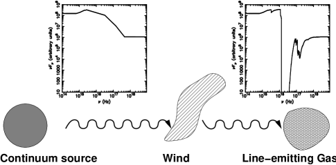
Figure 2.: A schematic illustration of the concept of “filtering”. The spectral energy distribution originates at the continuum source (left) and transverses the wind (center) that responds by emitting blueshifted lines. The transmitted continuum then illuminates gas emitting the intermediate- and low-ionization lines (right). Because the helium continuum is missing, the characteristic ionization of the lines is lower than it would have been without filtering.

We observed two NSL1s, IRAS 13224$-$3809 and 1H 0707$-$495, using HST in 1999 (Leighly & Moore 2004). The spectra are characterized by very blue continua; broad, strongly blueshifted high-ionization lines (including C IV and N V); and narrow, symmetric intermediate- (including C III], Si III], and Al III), and low-ionization (e.g., Mg II) lines centered at the rest wavelength. As discussed in §2, high-ionization lines are commonly blueshifted with respect to intermediate- and low-ionization lines, but these two objects exhibited an extreme example of this phenomenon in which the lines are almost completely decoupled. The emission-line profiles suggest that the high-ionization lines are produced in a wind and that the intermediate- and low-ionization lines are produced in low-velocity gas associated with the accretion disk or base of the wind. The highly asymmetric profile of C IV suggested that it is dominated by emission from the wind, so we developed a template from the C IV line. We modeled the bright emission lines in the spectra using a combination of this template and a narrow symmetric line centered at the rest wavelength (Leighly & Moore 2004).

Next, photoionization modeling using Cloudy was performed for the broad blueshifted wind lines and the narrow, symmetric, rest-wavelength-centered disk lines separately (for details, see Leighly 2004). A broad range of physical conditions was explored for the wind component, and a figure of merit was used to quantitatively evaluate the simulation results. The wind lines were characterized by relatively strong N V and 1400Å feature, but weak C IV feature. At first glance, this was difficult to explain because C IV falls between the other two in terms of ionization potential. A somewhat X-ray weak continuum and elevated metallicity produced an acceptable model for a broad range of densities $\log n\sim 7-11$) and ionization parameters ($\log U\sim-1.2$ to $-0.2$) and a small column density of $\log N_{H}\sim 21.4$. These parameters work because the lower X-ray flux reduces heating, and the higher metallicity allows the gas to cool more efficiently, allowing C IV and O IV] (a component of the 1400Å feature) to remain strong in the region of parameter space where N V is strong.

We then constructed a photoionization model for the intermediate- and low-ionization “disk” lines. The disk lines include C III] and Si III], so the density could be constrained. The C IV line had little kinematic overlap with the intermediate- and low-ionization lines. This seemed to imply that the ionization state of the gas was rather low ($\log U\sim-3$), so that it would not produce narrow C IV), which in turn placed the emitting gas at a very large distance from the central engine that seemed incompatible with the width of the lines. However, we realized that the radius of the disk-line-emitting gas would be smaller if the continuum were first transmitted through the wind before it illuminated the gas emitting those lines. The concept is illustrated in Fig. 2. Transmission through the wind removes the photons in the helium continuum, and therefore naturally reduces the C IV and other high-ionization line emission from the disk component. We found that we could produce the observed lines with a much larger ionization parameter of $\log U\sim-2.1$, and thus with a radius smaller by a factor of $\sim 2.8$, and a velocity width larger by a factor of $\sim 1.7$.

As discussed by Leighly (2004) the concept of filtering may be quite general. For example, filtering may explain why objects with blueshifted high-ionization lines have strong low-ionization lines such as Si II (Wills et al. 1999). It may explain the stronger Fe II emission in BALQSOs (Weymann et al. 1991). In addition, since the characteristic line-emission radius is reduced, it could skew black-hole mass estimates.

Acknowledgments.

KML and DC thank the organizers for the opportunity to present this review. Part of the work in writing this talk and review was done while KML was on sabbatical at the Department of Astronomy at The Ohio State University, and she thanks the members of the department for their hospitality. KML and DC acknowledge NNG05GB38G, NNG05GD73G and NNG05GD01G for support.

References

- Arav & Li (1994) Arav, N., & Li, Z.-Y. 1994, ApJ, 427, 700
- Baldwin et al. (1995) Baldwin, J., Ferland, G., Korista, K., & Verner, D. 1995, ApJ, 455, L119
- Baldwin & Netzer (1978) Baldwin, J. A., & Netzer, H. 1978, ApJ, 226, 1
- Baskin & Laor (2005) Baskin, A., & Laor, A. 2005, MNRAS, 356, 1029
- Boroson & Green (1992) Boroson, T. A., & Green, R. F. 1992, ApJS, 80, 109
- Bottorff al. (2000) Bottorff, M., Ferland, G., Baldwin, J., & Korista, K. 2000, ApJ, 542, 644
- Brotherton et al. (2001) Brotherton, M. S., Tran, H. D., Becker, R. H., Gregg, M. D., Laurent-Muehleisen, S. A., & White, R. L. 2001, ApJ, 546, 775
- Casebeer, Leighly & Baron (2006) Casebeer, D. A., Leighly, K. M., & Baron, E. 2006, ApJ, 637, 157
- Collin-Souffrin & Lasota (1988) Collin-Souffrin, S., & Lasota, J.-P. 1988, PASP, 100, 1041
- Dietrich et al. (2002) Dietrich, M., Hamann, F., Shields, J. C., Constantin, A., Vestergaard, M., Chaffee, F., Foltz, C. B., & Junkkarinen, V. T. 2002, ApJ, 581, 912
- Dhanda et al. (2006) Dhanda, N., Baldwin, J. A., Bentz, M. C., & Osmer, P. S. 2007, astro-ph/0612610
- Ferland et al. (1992) Ferland, G. J., Peterson, B. M., Horne, K., Welsh, W. F., & Nahar, S. N. 1992, ApJ, 387, 95
- Ferland et al. (1996) Ferland, G. J., Baldwin, J. A., Korista, K. T., Hamann, F., Carswell, R. F., Phillips, M., Wilkes, B., & Williams, R. E. 1996, ApJ, 461, 683
- Francis et al. (1991) Francis, P. J., Hewett, P. C., Foltz, C. B., Chaffee, F. H., Weymann, R. J., & Morris, S. L. 1991, ApJ, 373, 465
- Hamann et al. (2002) Hamann, F., Korista, K. T., Ferland, G. J., Warner, C., & Baldwin, J. 2002, ApJ, 564, 592
- Korista & Goad (2000) Korista, K. T., & Goad, M. R. 2000, ApJ, 536, 284
- Krolik & Kallmann (1988) Krolik, J. H., & Kallman, T. R. 1988, ApJ, 324, 714
- Kwan & Krolik (1981) Kwan, J., & Krolik, J. H. 1981, ApJ, 250, 478
- Leighly (2004) Leighly, K. M. 2004, ApJ, 611, 125
- Leighly & Moore (2004) Leighly, K. M., & Moore, J. R. 2004, ApJ, 611, 107
- Leighly et al. (2001) Leighly, K. M., Halpern, J. P., Helfand, D. J., Becker, R. H., & Impey, C. D. 2001, AJ, 121, 2889
- Leighly et al. (2007a) Leighly, K. M., Halpern, J. P., Jenkins, E. B., Grupe, D., Choi, J., & Prescott, K. B. 2007, ApJ, in press (astro-ph/0611349)
- Leighly et al. (2007b) Leighly, K. M., Halpern, J. P., Jenkins, E. B., & Casebeer, D. 2007, ApJ, submitted
- Murray et al. (1995) Murray, N., Chiang, J., Grossman, S. A., & Voit, G. M. 1995, ApJ, 451, 498
- Nagao, Marconi & Maiolino (2006) Nagao, T., Marconi, A., & Maiolino, R. 2006, å, 447, 157
- Puchnarewicz et al. (1995) Puchnarewicz, E. M., Mason, K. O., Siemiginowska, A., & Pounds, K. A., 1995, MNRAS, 276, 20
- Rees, Netzer, & Ferland (1989) Rees, M. J., Netzer, H., & Ferland, G. J. 1989, ApJ, 347, 640
- Shields et al. (1995) Shields, J. C., Ferland, G. J., & Peterson, B. M. 1995, ApJ, 441, 507
- Snedden & Gaskell (1999) Snedden, S. A., & Gaskell, C. M. 1999, ApJ, 521, L91
- Steffen et al. (2006) Steffen, A. T., Strateva, I., Brandt, W. N., Alexander, D. M., Koekemoer, A. M., Lehmer, B. D., Schneider, D. P., & Vignali, C. 2006, AJ, 131, 2826
- Vanden Berk et al. (2001) Vanden Berk, D. E., et al. 2001, AJ, 122, 549
- Weymann et al. (1991) Weymann, R. J., Morris, S. L., Foltz, C. B., & Hewitt, P. C. 1991, ApJ, 373, 23
- Williams (1971) Williams, R. E. 1971, ApJ, 167, L27
- Wills et al. (1999) Wills, B. J., Laor, A., Brotherton, M. S., Wills, D., Wilkes, B. J., Ferland, G. J., & Shang, Z. 1999, ApJ, 515, L53
- Zheng (1992) Zheng, W. 1992, ApJ, 385, 127
- Zheng et al. (1997) Zheng, W., Kriss, G. A., Telfer, R. C., Grimes, J. P., & Davidsen, A. F. 1997, ApJ, 475, 469