Virgo cluster early-type dwarf galaxies with the Sloan Digital Sky Survey.
III. Subpopulations: distributions, shapes, origins

Abstract

From a quantitative analysis of 413 Virgo cluster early-type dwarf galaxies (dEs) with Sloan Digital Sky Survey imaging data, we find that the dE class can be divided into multiple subpopulations that differ significantly in their morphology and clustering properties. Three dE subclasses are shaped like thick disks and show no central clustering: (1) dEs with disk features like spiral arms or bars, (2) dEs with central star formation, and (3) ordinary, bright dEs that have no or only a weak nucleus. These populations probably formed from infalling progenitor galaxies. In contrast, ordinary nucleated dEs follow the picture of classical dwarf elliptical galaxies in that they are spheroidal objects and are centrally clustered like E and S0 galaxies, indicating that they have resided in the cluster since a long time, or were formed along with it. These results define a morphology-density relation within the dE class. We find that the difference in the clustering properties of nucleated dEs and dEs with no or only a weak nucleus is not caused by selection biases, as opposed to previously reported suggestions. The correlation between surface brightness and observed axial ratio favors oblate shapes for all subclasses, but our derivation of intrinsic axial ratios indicates the presence of at least some triaxiality. We discuss possible interrelations and formation mechanisms (ram-pressure stripping, tidally induced star formation, harassment) of these dE subpopulations.

1. Introduction

As the most numerous type of galaxy in clusters, early-type dwarf galaxies are ideal probes to study the physical processes that govern galaxy formation and evolution in environments of different density. The pronounced morphology-density relation (e.g., Dressler, 1980; Binggeli et al., 1987) suggests that early-type dwarfs were either formed mainly in high-density environments, or originate from galaxies that fell into a cluster and were morphologically transformed. However, the actual formation mechanisms are still a matter of debate (see Jerjen & Binggeli, 2005, and references therein). Most of the proposed scenarios are based on the vigorous forces acting within a cluster environment, like ram-pressure stripping (Gunn & Gott, 1972) of dwarf irregular (dIrr) galaxies (e.g., van Zee et al., 2004), tidally induced star formation in dIrrs (Davies & Phillipps, 1988), or so-called harassment (Moore et al., 1996) of infalling late-type spirals through close encounters with massive cluster members.

Early-type dwarfs form a rather heterogeneous class of objects. In addition to the classical dwarf ellipticals, Sandage & Binggeli (1984) introduced the class of dwarf S0 (dS0) galaxies, which were conjectured to have disk components, based on signatures like high flattening or a bulge+disk-like profile (Binggeli & Cameron, 1991). The identification of spiral substructure then provided the first direct proof for a disk in an early-type dwarf (Jerjen et al., 2000), which, however, had not been classified as dS0 but as dwarf elliptical. Inspired by similar discoveries (e.g., Barazza et al., 2002; Graham et al., 2003; De Rijcke et al., 2003), we performed a search for disk features in 410 Virgo cluster early-type dwarfs (Lisker et al., 2006a, hereafter Paper I). We thereby included galaxies classified as dwarf elliptical and as dS0 to avoid any preselection bias, and assigned them the common abbreviation “dE”, which we adopt for this Paper as well. We identified disk features in 36 dEs, and argued that they constitute an unrelaxed population of disk-shaped galaxies different from the classical dwarf ellipticals (Paper I).

But the dE class shows yet more diversity: nucleated and non-nucleated dEs have different clustering properties (van den Bergh, 1986; Ferguson & Sandage, 1989), their flattening distributions differ (Binggeli & Cameron 1991; Ryden & Terndrup 1994; Binggeli & Popescu 1995), and color differences were reported as well (Rakos & Schombert, 2004; Lisker et al., 2005). Moreover, several of the bright dEs display blue central regions caused by recent or ongoing star formation (Lisker et al., 2006b, hereafter Paper II), and also differ in their spatial and flattening distributions from the bulk of dEs. Thus, prior to discussing possible formation mechanisms, we need to systematically disentangle the various dE subclasses observationally. This is the purpose of this Paper.

2. Sample selection

While our dE sample selection was already described in Papers I and II of this series, these studies were still based on the Data Release 4 of the Sloan Digital Sky Survey (SDSS; Adelman-McCarthy et al., 2006). Since we are now using the full SDSS Data Release 5 (DR5, Adelman-McCarthy et al., 2007) dataset, we provide here a detailed, updated description of our selection.

2.1. Selection process

The Virgo Cluster Catalog (VCC, Binggeli et al., 1985), along with revised classifications from Barazza et al. (2002, VCC 1422), Barazza et al. (2003, VCC 0850), and Geha et al. (2003, VCC 1488), contains 1197 galaxies classified “dE” or “dS0”, including candidates, that are certain or possible cluster members according to Binggeli et al. (1985), Binggeli et al. (1993), and Paper II. 552 of these fall within our chosen limit in apparent B magnitude from the VCC of $m_{\mathrm{B}}\leq 18.0$ mag (see Paper I). This is the same magnitude limit up to which the VCC was found to be complete (Binggeli et al., 1985). When adopting a Virgo cluster distance of $d=15.85\rm{Mpc}$, i.e., a distance modulus $m-M=31.0$ mag (see, e.g., Ferrarese et al., 2000), which we use throughout, this corresponds roughly to a limit in absolute magnitude of $M_{\mathrm{B}}\leq-13.0$ mag.

Six galaxies are not covered by the SDSS. While we initially included objects with uncertain classification (e.g., “dE?”), we then excluded all 50 galaxies that appeared to be possible dwarf irregulars from visual inspection of the coadded SDSS $g$,r, and $i$ images (see Paper I), or were classified as “dE/Im”. Three more objects (VCC 0184, 0211, and 1941) were excluded because they appear to be probable background spirals. Finally, VCC 1667 could not be classified properly, since it is significantly blended with multiple other galaxies. This leads to a final dE sample of 492 certain or possible cluster members, containing 426 certain cluster members on which we focus in the present Paper.

2.2. Presence of nuclei

While our classification of nucleated and non-nucleated dEs relies on the VCC, it is known from HST observations that many apparently non-nucleated dEs actually host a faint nucleus hardly detectable with ground-based imaging (Côté et al., 2006, also see Lotz et al. 2004b). A direct comparison of the VCC classification with the results from Côté et al. (2006) shows that, as a rough rule of thumb, the detection of dE nuclei in the VCC becomes incomplete for nucleus magnitudes that are fainter than the respective value of the host galaxy’s central surface brightness, measured within a radius $r=0.1^{\prime\prime}$ (Fig. 1). Our non-nucleated dEs could thus be more appropriately termed dEs without a nucleus of significant relative brightness as compared to the underlying light of the galaxy’s center. In fact, Grant et al. (2005) suggested that dEs classified as nucleated and non-nucleated might actually form a continuum of dEs with respect to relative nucleus brightness. Therefore, the VCC classification basically translates into probing opposite sides of this continuum — and this is exactly what makes it useful for our study of dE subclasses. If the relative brightness of a nucleus depends on its host galaxy’s evolutionary history, then one might expect nucleated and “VCC-non-nucleated” dEs to exhibit different population properties.

3. Data

The SDSS DR5 covers all VCC galaxies except for an approximately $2\arcdeg\times 2\fdg 5$ area at $\alpha\approx 186\fdg 2$, $\delta\approx+5\fdg 0$. It provides reduced images taken in the $u$, $g$, $r$, $i$, and $z$ bands with an effective exposure time of $54\rm{s}$ in each band (see also Stoughton et al., 2002), as well as the necessary parameters to flux calibrate them. The pixel scale of $0\farcs 396$ corresponds to a physical size of $30$ pc at our adopted Virgo cluster distance of $d=15.85\rm{Mpc}$. The SDSS imaging camera (Gunn et al., 1998) takes data in drift-scanning mode nearly simultaneously in the five photometric bands, and thus combines very homogeneous multicolor photometry with large area coverage and sufficient depth to enable a systematic analysis of dEs. The images have an absolute astrometric accuracy of $rms\leq 0\farcs 1$ per coordinate, and a relative accuracy between the $r$ band and each of the other bands of less than $0.1$ pixels (Pier et al., 2003). They can thus easily be aligned using their astrometric calibration and need not be registered manually.

The $rms$ of the noise per pixel corresponds to a surface brightness of approximately $24.2$ mag arcsec^-2 in the u-band, $24.7$ in $g$, $24.4$ in $r$, $23.9$ in $i$, and $22.4$ in z. The typical total signal-to-noise ratio (S/N) of a bright dE ($m_{\mathrm{B,VCC}}\approx 14$) amounts to about $1000$ in the r-band within an aperture radius of approximately two half-light radii. For a faint dE ($m_{\mathrm{B}}\approx 18$) this value is typically about $50$. While the S/N in the $g$ and i-band is similar, it is several times lower in the z-band and more than ten times lower in the u-band.

The SDSS provides photometric measurements for our galaxies, but we found these to be incorrect in many cases (Lisker et al., 2005). The SDSS photometric pipeline significantly overestimates the local sky flux around the Virgo dEs due to their large apparent sizes and low surface brightness outskirts. This affects the derivation of isophotal and Petrosian radii, the profile fits, and subsequently the calculation of total magnitudes, which can be wrong by up to 0.5 mag. For this reason, we used $B$ magnitudes from the VCC throughout the first two papers of this series. In the meantime, we have performed our own structural and photometric measurements (see Sect. 4), which we shall use here as well as in future papers of this series. Still, when we refer to $B$ magnitudes, these were adopted from the VCC.

Heliocentric velocities for part of the sample are provided by the NASA/IPAC Extragalactic Database (NED; also see Paper II for more detailed references).

4. Image preparation and analysis

4.1. Sky subtraction

The sky level on the SDSS images can vary by some tenths of the noise level across an image. For a proper determination of Petrosian radii of the dEs (see Sect. 4.3) despite their low surface brightness outskirts, it is thus not always sufficient to subtract only a single sky flux value from each SDSS image. Therefore, we performed sky subtraction through the following procedure. First, we constructed object masks for each SDSS image from the so-called segmentation images of the Source Extractor software (Bertin & Arnouts, 1996) by expanding these through smoothing with a Gaussian filter (using IRAF, Tody 1993). A preliminary sky level was then determined for each image as the median of all unmasked pixels, clipped three times iteratively at $3\sigma$. In order to reach a higher S/N than that of the individual images, we then produced a coadded image by summing the (weighted) $g$, $r$, and i-band images as described in Paper I. We then obtained an improved object mask from the coadded image and used this to refine our sky level measurement.

Finally, the sky flux distribution across the image was determined by computing the average flux – clipped five times iteratively at $3\sigma$ – of all unmasked pixels in 201$\times$201 pixel boxes, centered every 40 pixels. This grid of values can be stored as a 52$\times$38 pixel “sky image”. Pixels in this sky image that did not contain useful values due to too many masked pixels in the parent image were linearly interpolated using IRAF fixpix. We then applied a 3$\times$3 pixel median filter to the sky image, expanded it to match its parent SDSS image’s size (using IRAF magnify with linear interpolation), and subtracted it from the latter. This yields the final $u$, $g$, $r$, $i$, and $z$ images.

We point out that there is, to our knowledge, no general agreement or recipe as to whether to use, e.g., the clipped mean, the median, the clipped median, or the mode, for determination of the sky level. However, it is advisable that the chosen approach be reconciled with the image measurements to be performed, which in our case is the derivation of Petrosian radii (see Sect. 4.3). Since the latter is based on the average flux within given annuli, we chose to use the clipped average flux of all unmasked pixels for our sky level measurement. This guarantees that the resulting flux level in each image is zero as “seen” by the Petrosian radius calculation.

4.2. Calibration and extraction

We calibrated the sky subtracted SDSS images using the provided flux calibration information (photometric zeropoint and airmass correction). We also corrected for the reported SDSS zeropoint offsets in the $u$ and $z$ bands from the AB system (Oke & Gunn, 1983, see http://www.sdss.org/dr5/algorithms/fluxcal.html). However, before working with the images, it is advantageous to put together adjacent images: a number of galaxies partly extend beyond the image edges and reappear on the corresponding neighbouring image. Bright dEs typically have apparent diameters of 300 pixels or more, which is rather large compared to the SDSS image size of 2048$\times$1489 pixels. The SDSS astrometric calibration allows us to accurately put together adjacent images, which we did before extracting an 801$\times$801 pixel cutout image for each galaxy. These cutout images were then corrected for Galactic extinction, using one value per image, calculated with the dust maps and corresponding software of Schlegel et al. (1998, provided at http://www.astro.princeton.edu/$\sim$schlegel/dust/data/). From the $g$, $r$, and $i$ cutout image we produced a final coadded image for each galaxy.

4.3. Morphology

We perform an iterative process of determining shape and total flux for each galaxy, as described below. Throughout this process, we mask disturbing foreground or background objects, i.e., we do not consider masked pixels in any calculation. We start with deriving the Petrosian radius (Petrosian, 1976), as defined by Stoughton et al. (2002), on the coadded image. Using a circular aperture with one Petrosian radius, we then find the center of the galaxy’s image by iteratively searching for the minimum asymmetry, following Conselice et al. (2000). The asymmetry $A$ is calculated as

$$A=\frac{\displaystyle\sum_{i}|f_{i}-f_{i,180}|}{\displaystyle\sum_{i}|f_{i}|},$$ (1)

where $f_{i}$ is the flux value of the i-th pixel, and $f_{i,180}$ is the flux value of the corresponding pixel in the 180-degree rotated image.

The asymmetry is computed using an initially guessed central position (from Paper I for objects in the SDSS DR4, and from visual examination for objects in DR5, using SAOImage DS9, Joye & Mandel 2003), as well as for using the surrounding eight positions in a 3$\times$3 grid as center. If one of the surrounding positions yields a lower asymmetry, it is adopted as new central position. This process is repeated until convergence. We perform two of these “asymmetry centerings”: a first one with a step size of 1 pixel, and a second one with a step size of 0.3 pixels. The initial and final value typically differ by less than a pixel.

We then compute the parameters defining an elliptical aperture (axial ratio and position angle) from the image moments (Abraham et al., 1994), and derive a “Petrosian semimajor axis” $a_{\mathrm{p}}$, i.e., we use ellipses instead of circles in the calculation of the Petrosian radius (see, e.g., Lotz et al., 2004a). Within this elliptical aperture with a semimajor axis $a$ of $1a_{\mathrm{p}}$, we perform another iteration to re-derive the elliptical shape parameters from the image moments, and also to re-derive $a_{\mathrm{p}}$.

The elliptical shape is then applied to measure the total flux in the $r$ band within an elliptical aperture with $a=2a_{\mathrm{p}}$, which also yields a half-light semimajor axis in $r$ ($a_{{\rm hl},r}$). Using this value for $a_{{\rm hl},r}$, we go back to the coadded image and fit an ellipse to the isophotal shape of the galaxy at $a=2a_{{\rm hl},r}$, using IRAF ellipse. The elliptical annulus used for the isophotal fit ranges from $2^{0.75}a_{{\rm hl},r}$ to $2^{1.25}a_{{\rm hl},r}$.

This new elliptical shape is now used to derive the final Petrosian semimajor axis on the coadded image, and to subsequently measure again the total flux in the $r$ band within $a=2a_{\mathrm{p}}$, yielding the final value for $a_{{\rm hl},r}$. The isophotal shape is then measured again at $a=2a_{{\rm hl},r}$, yielding the axial ratio that we shall use throughout this Paper.

Since we masked disturbing foreground or background objects by not considering their pixels, our measured total flux for a given galaxy is always lower than it would be without any such “holes” in the galaxy’s image. In order to correct for this effect, we subdivide the final aperture of each galaxy into 20 elliptical annuli of equal width, and assign each masked pixel the average flux value of its respective annulus. This yields our final value for the total $r$ band flux and the corresponding magnitude. The difference to the uncorrected value is typically less than 0.1 mag.

For 13 of our dEs, the derivation of the Petrosian radius did not converge, due to the fact that these galaxies sit within the light of nearby bright sources. While in some of these cases, it would still be possible to “manually” define an axial ratio for the galaxy, we decided to exclude these objects from our sample, since no reliable $r$ band magnitudes can be derived, which are needed for our definitions of dE subclasses in Sect. 5. This leaves us with a working sample of 413 Virgo cluster dEs.

5. Early-type dwarf subclasses

5.1. Subclass definitions

Of our 413 Virgo dEs, 37 display disk features, like spiral arms, bars, or signs of an edge-on disk (Paper I, adding VCC 0751 to the objects listed there in order to update to SDSS DR5). We term these objects “dE(di)s”, and separate this dE subclass from the ordinary, “featureless” dEs (Fig. 2). In order to further explore the diversity of the latter, we perform a secondary subdivision into nucleated (“dE(N)”) and non-nucleated (“dE(nN)”) galaxies, based on the identification of nuclei in the VCC as outlined in Sect. 2.2. Since a further subdivision of the dE(di)s would lead to statistically insignificant subsamples, we shall instead discuss their nucleated fraction in the text. Finally, since our galaxies span a range of almost 5 mag in $r$, it appears worth performing a tertiary subdivision into dEs brighter and fainter than the median $r$ brightness of our full sample, namely $m_{\mathrm{r}}=15.67$ mag. Moreover, all but three of the dE(di)s are brighter than this value; thus our subdivision allows us to compare them to ordinary dEs of similar luminosities. The percentage of each subsample among our full sample of 413 dEs is given in parentheses in Fig. 2, whereas the actual number of galaxies contained in each subsample is given in the left column of Fig. 3.

The subclasses defined so far are based on structural properties only — for morphological classification of galaxies, it is not advisable to use color information. However, in Paper II we identified a significant number of dEs with blue centers (17 galaxies, including VCC 0901 from the SDSS DR5). These objects, termed “dE(bc)s”, exhibit recent or ongoing central star formation, similar to NGC 205 in the Local Group. They were morphologically classified as dwarf ellipticals or dS0s by Sandage & Binggeli (1984), and their regular, early-type morphology was confirmed in Paper II; thus, they are not possible irregular galaxies, which we have excluded from our samples here and in previous papers of this series. The flattening distribution of the dE(bc)s was found to be incompatible with intrinsically spheroidal objects (Paper II), and their distribution with respect to local projected density suggests that they are an unrelaxed population. The latter result is similar to the spatial distribution of Virgo and Fornax dwarfs with early-type morphology that are gas-rich and/or show star formation (Drinkwater et al., 2001; Conselice et al., 2003; Buyle et al., 2005).

While it is not clear a priori that any of the dE subclasses defined above are evolutionary interrelated, each dE(bc) unavoidably evolves into one of the above dE types once star formation ceases and the central color reddens (Paper II). Therefore, and because the dE(bc)s are defined through color instead of morphological properties, we do not consider them a morphological dE subclass. On the other hand, their star formation and presence of gas (Paper II) might imply that their formation process is not completely finished yet. It thus appears more cautious to separate them from the rest of dEs (see Fig. 2) in order to not bias the population properties of the other subclasses. In the discussion (Sect. 7) we try to assess which dE type(s) the dE(bc)s could possibly evolve into. Note that four objects are common to both the dE(di) and the dE(bc) sample. We exclude these from the sample of dE(di)s, which now comprises 33 galaxies. Table 1 lists our dEs along with their subclass.

A similar subdivision of the dE class into bright and faint (non-)nucleated subsamples was performed by Ferguson & Sandage (1989), also with the aim of studying shapes and spatial distributions of the resulting subsamples. Our subdivision is different in two respects: first, Ferguson & Sandage defined all galaxies with $m_{\mathrm{B}}<17.5$ mag as “bright”, whereas our magnitude separation (at $m_{\mathrm{r}}=15.67$ mag) is done at significantly brighter values and divides our full sample into equally sized halves. Second, we have the advantage of excluding dE(di)s and dE(bc)s from the “normal” dEs, thereby obtaining cleaner subsamples, especially for the bright objects: all but three of the dE(di)s are brighter than $m_{\mathrm{r}}=15.67$ mag.

While Ferguson & Sandage (1989) found statistically significant differences in the spatial distributions of their subsamples – with dE(N)s being much more centrally clustered than the bright dE(nN)s – their flattening distributions were only based on eye-estimated axial ratios from photographic plates. These can be uncertain by $\sim$20% (Ferguson & Sandage, 1989). With our measured axial ratios from the coadded SDSS images at hand, we therefore present in the following subsection a more detailed and accurate study of the flattening distributions of the different dE subsamples, and attempt to deduce their approximate intrinsic shapes.

5.2. Subclass shapes

From the axial ratio measurements of our galaxies (Sect. 4.3), we put together the flattening distributions of each dE subsample. These are presented in the second column of Fig. 3 as running histograms, i.e., at each sampling point we consider the number of objects within a bin of constant width, and normalize the resulting curve to an area of 1. The bin width is 0.15, which we have chosen to be one fifth of the range in axial ratio covered by our galaxies. The sampling step is 0.04 (one quarter of the bin width). The bright and faint dE(N)s, and also the faint dE(nN)s, predominantly have rather round apparent shapes, while the bright dE(nN)s, dE(di)s, and dE(bc)s exhibit a significant fraction of objects with rather flat apparent shapes.

Since the division between bright and faint objects at $m_{\mathrm{r}}=15.67$ mag is somewhat arbitrary, we test whether the difference between the axial ratio distributions of faint and bright dE(nN)s becomes even more pronounced if a wider magnitude separation is adopted. The grey curves in the respective panels of the second column of Fig. 3 show the distributions for bright dE(nN)s with $m_{\mathrm{r}}\leq 15.67-0.5$ mag (23 objects) and for faint dE(nN)s with $m_{\mathrm{r}}\leq 15.67+0.5$ mag (86 objects). While the faint dE(nN)s basically remain unchanged, the bright dE(nN)s indeed tend slightly towards flatter shapes, but the difference is rather small.

A statistical comparison of the axial ratio distributions of our dE subsamples confirms what is seen in Fig. 3: a K-S test yields very low probabilities that any of the “flatter” subsamples (bright dE(nN)s, dE(di)s, and dE(bc)s, lower three rows) could stem from the same true distribution function as any of the “rounder” subsamples (bright and faint dE(N)s as well as faint dE(nN)s, upper three rows). This confirms our findings from Papers I and II for the dE(di)s and dE(bc)s, respectively. The resulting probabilities from the K-S test for the pairwise comparison of the subsamples are given as percentages in Fig. 4. Interestingly, the lowest probability of all comparisons is obtained when matching the distributions of bright and faint dE(nN)s: here, the probability of the null hypothesis that they stem from the same underlying distribution function is only 0.10%. Note that the probabilities for the comparison of the “flatter” subsamples with the “rounder” ones increase slightly with decreasing sample size, going from the bright dE(nN)s to the dE(di)s and then to the dE(bc)s. However, the probability for a common underlying distribution of dE(bc)s and the bright and faint dE(N)s is still only 3.8% and 4.6%, respectively.

Is it possible to deduce the distributions of intrinsic axial ratios from those of the apparent ones? As discussed in detail by Binggeli & Popescu (1995), the intrinsic shapes can be deduced when assuming that they are purely oblate or purely prolate. The distribution function $\Psi$ of intrinsic axial ratios $q$ can then be derived from the distribution function $\Phi$ of observed axial ratios $p$ through (Fall & Frenk 1983, eqs. (6) and (9))

$$\Psi(q)=\frac{2}{\pi}\sqrt{1-q^{2}}\frac{d}{dq}\int_{0}^{q}dp\frac{\Phi(p)}{\sqrt{q^{2}-p^{2}}}$$ (2)

for the oblate case, and

$$\Psi(q)=\frac{2}{\pi}\frac{\sqrt{1-q^{2}}}{q^{2}}\frac{d}{dq}\int_{0}^{q}dp\frac{p^{3}\Phi(p)}{\sqrt{q^{2}-p^{2}}}$$ (3)

for the prolate case. Following Binggeli & Popescu (1995), we first defined adequate analytic functions $\Phi(p)$ that represent the observed distributions, and then evaluated the above equations numerically. The analytic “model functions” are shown in the third column of Fig. 3; they were constructed from combinations of (skewed) Gaussians with each other and, in some cases, with straight lines. Note that, for the dE(bc)s, we decided not to follow the observed distribution in all detail, since it is drawn from a rather small sample of 17 galaxies, which probably is the cause of the fluctuations seen.

The deduced intrinsic distributions are presented in the fourth column of Fig. 3, for the oblate (grey lines) and prolate (black dash-dotted lines) case. We also show 3-D illustrations of the galaxy shapes for each distribution (fifth column), using in each case the axial ratio of the 25th percentile (left 3-D plot) and the 75th percentile (right 3-D plot). These results confirm that the bright dE(nN)s, dE(di)s, and dE(bc)s do have lower axial ratios than the bright and faint dE(N)s and the faint dE(nN)s. Furthermore, we point out that the bright and faint dE(N)s span a rather wide range of intrinsic axial ratios, and are, on average, somewhat flatter than what was deduced by Binggeli & Popescu (1995): our median value (see the 3-D illustrations in Fig. 2) is slightly flatter than E3 for the prolate case, and slightly flatter than E4 for the oblate case.

Can we decide whether the true shapes of our galaxies are more likely to be oblate or to be prolate? For this purpose, we make use of the surface brightness test (Marchant & Olson, 1979; Richstone, 1979), again following Binggeli & Popescu (1995). If dEs were intrinsically oblate spheroids, galaxies that appear round would be seen face-on and should thus have a lower mean surface brightness than galaxies that appear flat; the latter would be seen edge-on. For the prolate case, the inverse relation should be observed. However, before we can perform this test, we need to take into account the strong correlation of dE surface brightness with magnitude (e.g., Binggeli & Cameron, 1991): if, by chance, the few apparently round galaxies in one of our smaller subsamples would happen to be fainter on average than the apparently flat ones, this could introduce an artificial relation of axial ratio with surface brightness. Therefore, instead of directly using surface brightness like earlier studies did, we use the surface brightness offset from the mean relation of surface brightness and magnitude. We plot these values, measured in the $r$ band within $a=2a_{{\rm hl},r}$, against axial ratio (measured at the same semimajor axis, see Sect. 4.3) for each dE subsample, shown in the rightmost column of Fig. 3. For all subsamples, a positive correlation of surface brightness offset with axial ratio can be seen, favoring the oblate model in agreement with earlier studies (e.g., Marchant & Olson, 1979; Richstone, 1979; Binggeli & Popescu, 1995). For the “rounder” subsamples (top three rows), some additional contribution by prolate objects might be “hidden” within the rather large scatter of surface brightness offsets at larger axial ratios. We denote these results in Fig. 3 by the arrows pointing from the surface brightness test diagram towards the favored intrinsic galaxy shapes. The arrow size represents the implied contribution from intrinsically prolate and oblate objects. Among the “flatter” subsamples (lower three rows), for which the oblate case is favored, the dE(di)s have the lowest axial ratios, with a median value of 0.33 (bright dE(nN)s: 0.42, dE(bc)s: 0.44). The galaxies in these subsamples are thus most likely shaped like thick disks.

The above considerations needed to be restricted to purely oblate and purely prolate shapes. However, for all subsamples, a small part of the deduced (and favored) intrinsic oblate distribution becomes negative at large axial ratios, trying to account for the low number of apparently round objects. This implies that most of the galaxies might actually have triaxial shapes, in accordance with the conclusions of Binggeli & Popescu (1995).

5.3. Subclass distribution within the cluster

While it has been known for some time that nucleated and non-nucleated dEs have different clustering properties (e.g., van den Bergh, 1986; Ferguson & Sandage, 1989), this statement has been challenged by Côté et al. (2006), who conjectured that it might just be the result of a selection bias in the VCC. It therefore appears worth to perform a quantitative comparison of the distributions of our dE subsamples within the cluster, and to then proceed with testing the issues raised by Côté et al. (2006) in detail.

The projected spatial distributions of our subsamples are shown in the middle column of Fig 5. While both bright and faint dE(N)s exhibit a rather strong central clustering, the faint dE(nN)s appear to be only moderately clustered, and the dE(di)s and dE(bc)s show basically no central clustering. The bright dE(nN)s even seem to be preferentially located in the outskirts of the cluster.

To put the above on a more quantitative basis, we present in Fig. 6 the cumulative distribution of each of our subsamples with respect to local projected density. Following Dressler (1980) and Binggeli et al. (1987), we define the latter for each galaxy as the number of objects per square degree within a circle that includes the ten nearest neighbours, independent of galaxy type. Only certain cluster members are considered. For comparison, we also show the same distributions for different Hubble types (Fig. 6, inset), i.e., for the rather strongly centrally clustered giant early-type galaxies, as well as for the weakly clustered and probably infalling spiral and irregular galaxies (e.g., Binggeli et al., 1987).

As a confirmation of the impression from the spatial distribution, the bright dE(nN)s are preferentially found in regions of moderate to lower density, similar to (and at even slightly lower densities than) the distribution of irregular galaxies, in accordance with the findings of Ferguson & Sandage (1989). This implies that they, as a population, are far from being virialized. The densities then increase slightly going from the bright dE(nN)s to the dE(bc)s, dE(di)s, and the faint dE(nN)s, in this order. Still, all of these are distributed similarly to the irregular and spiral galaxies in the cluster, again implying that they are unrelaxed or at least largely unrelaxed galaxy populations, and confirming the impression from their projected spatial distribution. In contrast, both bright and faint dE(N)s are located at larger densities, and display a distribution comparable to the E and S0 galaxies, in agreement with the results of Ferguson & Sandage (1989). This would suggest that they are a largely relaxed or at least partially relaxed population. Note, however, that the Es alone (without the S0s) are located at still higher densities. Conselice et al. (2001) pointed out that only the Es appear to be a relaxed galaxy population, while all others, including the S0s, are not — thus, the dE(N)s presumably are not fully relaxed either.

We performed statistical pairwise comparisons of the distributions of our dE subsamples with respect to density, similar as for the axial ratios in Sect. 5.2. The K-S test probabilities for the null hypothesis that two observed distributions stem from the same underlying distribution are given as percentages in Fig. 7. Even though the faint dE(nN)s are, among the “lower-density” subsamples, closest to the bright and faint dE(N)s, their probability for having the same underlying distribution is 0.08 and 0.07%, respectively. These probabilities are higher for the dE(di)s and dE(bc)s: although they are located at even lower densities, their rather small sample sizes let the probability increase as compared to that of the faint dE(nN)s. Finally, the bright dE(nN)s are located at such low densities that their K-S test comparison with the dE(N)s yields a probability of 0.00%, and that even the comparison with the faint dE(nN)s only yields a probability of 3.7% for them having the same true distribution. Given the morphological differences between the subsamples, as deduced in Sect. 5.2, Fig. 6 basically shows a morphology-density relation within the dE class.

This view appears to be corroborated by the distributions of heliocentric velocities (right column of Fig. 5) of the dE subsamples: that of the bright dE(N)s has a single peak and is fairly symmetric, while especially the faint dE(nN)s, dE(di)s, and dE(bc)s display rather asymmetric distributions with multiple peaks. The latter could be interpreted as being a signature of infalling populations (Tully & Shaya 1984; Conselice et al. 2001). However, the differences between these velocity distributions are not or only marginally significant — the “most different” pair of distributions according to the K-S test are the bright dE(nN)s and the dE(bc)s, which have a probability of 6.6% for the null hypothesis. The main issue here are the small sample sizes: only a fraction of the galaxies of each subsample has measured velocities (numbers are given in parentheses in the left column of Fig. 5), which are available from the NED for 193 of our 413 dEs, and, e.g., for only 19 of our 39 bright dE(nN)s. Similarly, measurements of the skew or kurtosis of the distributions do not yield values that differ significantly from zero. We can thus only state that the rather asymmetric, multi-peaked distributions of the faint dE(nN)s, the dE(di)s, and the dE(bc)s would be consistent with our above conclusion that they are mostly unrelaxed populations, but that more velocity data is needed to perform a reliable quantitative comparison of velocity distributions.

5.4. Remarks on possible selection biases

The different spatial distribution of dE(N)s and dE(nN)s was long considered a fundamental and well-founded observation, but has recently been questioned by Côté et al. (2006). These authors argued that galaxies with high central surface brightness (HSB, with $\mu_{\rm g,central}\lesssim 20$ mag arcsec^-2 or $B\lesssim 14.55$) would have been preferentially classified as non-nucleated in the VCC, which may have lead to a selection bias in the VCC that artificially relates spatial distribution to nucleus presence. We test this conjecture by considering the following points:

(1) If the dE(nN)s were objects in which nuclei have preferentially gone undetected due to a too large central surface brightness, the dE(nN)s’ surface brightnesses should, on average, be significantly higher than those of the dE(N)s. However, the mean surface brightness in $r$ within the half-light aperture has very similar median values for the bright dE(nN)s ($\mu_{r}=22.65$ mag arcsec^-2) and the bright dE(N)s ($\mu_{r}=22.63$ mag arcsec^-2), which makes such a bias unlikely. Furthermore, the distributions of surface brightnesses of the two subsamples are similar — a K-S test yields a probability of 84% for the null hypothesis that they stem from the same underlying distribution. Certainly, measurements of the very central surface brightness, which are possible only with high-resolution observations, would provide a more direct argument here. However, since both nucleated and non-nucleated dEs within a given magnitude range have similar surface brightness profiles (Binggeli & Cameron, 1991), their effective surface brightness and central surface brightness are closely correlated.

(2) Only one single galaxy among our 39 bright dE(nN)s (2.5%) is bright enough to fall among Côté et al.’s definition of a HSB dE. In contrast, 14 of our 121 bright dE(N)s (12%) would qualify as HSB dE. Therefore, it appears highly unlikely that a significant number of dE(nN)s possess nuclei with similar relative brightnesses as those of the dE(N)s that were not detected by Binggeli et al. (1985).

(3) None of the dEs in Côté et al.’s own sample that were previously classified as non-nucleated, but have now been found to host a weak nucleus, actually are HSB dEs.

(4) Since we are interested in the distributions of our subsamples with respect to density in the cluster, we translate Côté et al.’s conjecture about the spatial distribution of the dEs into one about the distribution with respect to density: if the different density distributions of bright dE(N)s and dE(nN)s (see above) would primarily be caused by a surface brightness selection effect, a significantly larger fraction of the high surface brightness objects should be located at lower densities as compared to the lower surface brightness objects. To test for this possible bias, we plot the mean $r$ band surface brightness within the half-light aperture against local projected density for the combined sample of bright dE(N)s and dE(nN)s (Fig. 8). No correlation is seen, ruling out that such a bias is present in our data.

We point out that it might of course still be the case that most of the dE(nN)s host weak nuclei that are below the VCC detection limit, as discussed in Sect. 2.2. However, what is at stake here is the question whether a significant number of dE(nN)s should already have been classified as dE(N)s by the VCC, and whether this could account for the population differences that we find. The above arguments clearly rule out such a bias. We can thus conclude that the bright dE(N)s and dE(nN)s are indeed distinct dE subpopulations that differ in their clustering properties (Figs. 6 and 7), as well as in their shapes (Figs. 3 and 4).

6. Color analysis

Since our morphological subdivision of the dEs into several subpopulations is now established, the next step would obviously be to compare their stellar population properties. Given that the SDSS imaged every galaxy in five bands, it should be able to provide some insight into their stellar content, even though it is basically impossible to disentangle ages and metallicities with optical broadband photometry alone. However, the issue is complicated by the fact that the $u$ and $z$ band images, which would be very important for an analysis of the stellar content, have a very low S/N (see Sect. 3). It is therefore important to perform a thorough study of the dE colors and color gradients that properly takes into account measurement errors and the different S/N levels for objects of different magnitudes and surface brightnesses. Such a study is beyond the scope of the present Paper and will be presented in a forthcoming Paper of this series.

Nevertheless, in order to tackle the question about whether the dE subsamples differ in their color properties, we present in Fig. 9 the inner $u-g$ (“age-sensitive”) versus $i-z$ (“metallicity-sensitive”) colors for the bright ($m_{\mathrm{r}}\leq 15.67$) dEs, measured within an aperture of $a=0.5a_{{\rm hl},r}$. This approach guarantees relatively small errors (typical values are shown in the lower left corner of the Figure) that need not be taken into account individually. For each dE subsample, we indicate its median color values with the black symbols drawn with thick lines.

However, a direct comparison of these values would be biased by the existence of a color-magnitude relation: if different subsamples had, on average, significantly different magnitudes, they would be offset in our color-color diagram even if they followed exactly the same color-magnitude relation. We therefore compute an approximate correction for this effect: first, we perform a linear least squares fit to the color-magnitude relations ($r$ versus $u-g$ and $r$ versus $i-z$) of our full dE sample, clipping one time at 3$\sigma$ and excluding the dE(bc)s because of their blue inner colors. We then derive the median $r$ magnitude of each subsample, and use the linear fit to compute its expected color offset from the sample of dE(nN)s, which we choose as reference. The so obtained corrected median colors are shown in Fig. 9 as black symbols drawn with thin lines, and are connected with lines to their uncorrected values.

The dE(bc)s exhibit, as expected, the bluest colors of all subsamples, basically by definition, since we focus here on the inner galaxy colors. While the corrected colors of the dE(di)s are similar to those of the dE(nN)s, the dE(N)s are, on average, redder in $i-z$ and significantly redder in $u-z$. Given the very small color correction and large sample size of the dE(N)s, this can be considered a robust result. In the inset shown in Fig. 9, we compare the median values of the dE(nN)s and dE(N)s to two model tracks from stellar population synthesis calculations (Bruzual & Charlot, 2003). Both tracks represent stellar populations formed through a single burst of star formation that exponentially decays with time ($\tau=0.5$ Gyr), using Padova 2000 isochrones and a Chabrier IMF. The tracks are curves of constant metallicity (grey solid line: $Z=0.008$, grey dotted line $Z=0.004$); ages increase from bottom to top and are marked at 3, 6, 10, and 14 Gyr (the latter mark is outside of the plot area for the $Z=0.008$ track). Our measured values lie along of the $Z=0.008$ track, illustrating that, within the framework of our simplified stellar population models, the color difference between dE(nN)s and dE(N)s could be interpreted as a difference in age. According to this simple approach, the dE(N)s would be, on average, a few Gyr older than the dE(nN)s. However, the measurements also fall roughly along a virtual line connecting the 6 Gyr points of each model, showing that they might also be interpreted as a difference in metallicity. While this color offset between the dE(N)s and dE(nN)s would be qualitatively consistent with the study by Rakos & Schombert (2004), who find the dE(N)s in the Coma and Fornax clusters to have older stellar populations than the dE(nN)s, reliable conclusions need to await a more comprehensive color study of our dEs.

7. Discussion

7.1. Interrelations between subclasses

The bright dE(nN)s and dE(di)s are both unrelaxed populations of relatively bright dEs shaped like thick disks. This also applies to the dE(bc)s, which could thus be candidates for being the direct progenitors of the former: the presently blue centers of the dE(bc)s will evolve to typical dE colors within 1 Gyr or less after the cessation of star formation (Paper II). Therefore, the bright dE(nN)s and dE(di)s could constitute those disk-shaped dEs where central star formation has already ceased. To test this hypothesis, we make the following considerations. There are 39 bright dE(nN)s, as well as 30 dE(di)s with $m_{\mathrm{r}}\leq 15.67$ mag, 7 of which are non-nucleated. This adds up to 69 “non-star-forming, disk-shaped dEs”, 23 (33%) of which are nucleated. Among the dE(bc)s there are 15 galaxies with $m_{\mathrm{r}}\leq 15.67$ mag, 6 (40%) of which are nucleated. Thus, the fraction of nucleated galaxies would be compatible with our hypothesis within the errors, with the caveat that nuclei might still form in the centers of some dE(bc)s (see Oh & Lin 2000 and Paper II), which would raise the nucleated fraction of the dE(bc)s.

Now, 43% of the non-star-forming, disk-shaped dEs are dE(di)s, i.e., show disk features (not only an overall disk shape). If the dE(bc)s would contain the same fraction of galaxies that display disk features, we would expect 6.5 such objects among the 15 dE(bc)s, with a standard deviation of 1.9. The observed number of 4 lies within 1.3 $\sigma$ of the expected value and could thus still be reconciled with the above picture. However, since not only the dE(di)s, but also the bright dE(nN)s are disk-shaped, why do the latter not display disk features like the dE(di)s? This could either indicate a correlation between the presence of a significantly bright nucleus and the presence of disk substructure, or it could imply that there is more than one formation path towards disk-shaped dEs.

7.2. Formation mechanisms

If dEs originated from galaxies that fell into the cluster, how long ago could this infall have taken place? Conselice et al. (2001) derived a two-body relaxation time for the Virgo dEs of much more than a Hubble time. Even violent relaxation, which could apply for the case of infalling or merging groups, would take at least a few crossing times $t_{\rm cr}$, with $t_{\rm cr}\approx 1.7$ Gyr for the Virgo cluster (Boselli & Gavazzi, 2006). Therefore, the majority of dE(N)s or their progenitors should have experienced infall in the earliest phases of the Virgo cluster (which is a rather young structure, see Binggeli et al. 1987 and Arnaboldi et al. 2004), or they could have formed in dark matter halos along with the cluster itself. All other dE subclasses are largely unrelaxed populations, implying that they have formed later than the dE(N)s, probably from (continuous) infall of progenitor galaxies. Our color analysis in Sect. 6 would support this view, since it finds that the inner colors of the dE(N)s can be interpreted with an older stellar population than the dE(nN)s. This would be expected if one assumes that the progenitor galaxies had been forming stars until their infall into the cluster, resulting in a younger stellar population on average in the case of a later infall (neglecting possible metallicity differences). However, as stressed in Sect. 6, robust conclusions need to await a more detailed multicolor study of our dEs.

The galaxy harassment scenario (Moore et al., 1996) describes the structural transformation of a late-type spiral into a spheroidal system through strong tidal interactions with massive cluster galaxies. A thick stellar disk may survive and form a bar and spiral features that can be retained for some time, depending on the tidal heating of the galaxy (Mastropietro et al., 2005). Harassment could thus form disk-shaped dEs, and dE(di)s in particular. Moreover, it predicts gas to be funneled to the center and form a density excess there (Moore et al., 1998), which would be well suited to explain the central star formation in the dE(bc)s. Therefore, it appears possible that harassment could form disk-shaped dEs that first appear as dE(bc)s and then passively evolve into dE(di)s and bright dE(nN)s as their star formation ceases (see Sect. 7.1). It might also provide a way to form the fainter non-nucleated dEs, assuming that the tidal forces have a stronger effect on the shape of less massive galaxies, resulting in rounder objects on average. However, in order to explain all these subclasses by a single process, one would need to invoke a correlation between the presence of a nucleus and of disk features, as discussed in Sect. 7.1.

Ram-pressure stripping (Gunn & Gott, 1972) of dwarf irregulars (dIrrs) could be responsible for the fact that the disk-shaped bright dE(nN)s do not show disk features like the dE(di)s: dIrrs typically have no nucleus, and ram-pressure stripping exerts much less perturbing forces than a violent process like harassment, thus probably not triggering the formation of bars or spiral arms. Commonly discussed problems with this scenario are the metallicity offset between dEs and dIrrs (Thuan, 1985; Richer et al., 1998; Grebel et al., 2003) and the too strong fading of dIrrs after cessation of star formation (Bothun et al., 1986). Also, the flattening distribution of Virgo cluster dIrrs – with intrinsic (primary) axial ratios $\geq$ 0.5 for most galaxies (Binggeli & Popescu, 1995) – is not quite like that of our bright dE(nN)s. On the other hand, significant mass loss due to stripped gas might affect the stellar configuration of the galaxies and could thus possibly account for the difference. Moreover, the flattening distribution of the dIrrs is similar to that of the faint dE(nN)s (cf. Fig. 9 of Binggeli & Popescu 1995), suggesting that these – and possibly not the bright dE(nN)s – might be stripped dIrrs.

Tidally induced star formation of dIrrs might be able to overcome the problems of the ram-pressure stripping scenario: the initially lower metallicity and surface brightness of a dIrr are increased by several bursts of star formation (Davies & Phillipps, 1988), during which the galaxy appears as blue compact dwarf (BCD). After the last BCD phase it fades to become a dE, thereby providing an explanation how BCDs could be dE progenitors, which has frequently been discussed (e.g., Bothun et al. 1986; Papaderos et al. 1996; Grebel 1997; Paper II). The last star formation burst might occur in the central region, consistent with the appearance of the dE(bc)s.

In addition to the number of possible formation scenarios, the role of the nuclei provides another unknown element. If dE(N)s and dE(nN)s would actually form a continuum of dEs with respect to relative nucleus brightness as suggested by Grant et al. (2005), their significantly different population properties could be interpreted with a correlation between relative nucleus brightness and host galaxy evolution. Such a correlation could, for example, be provided by nucleus formation through coalescence of globular clusters (GCs): the infall and merging of several GCs – resulting in a rather bright nucleus like in a dE(N) – takes many Gyr (Oh & Lin, 2000), consistent with the dE(N)s being in place since long. The dE(nN)s, on the other hand, were probably formed more recently, leaving time for only one or two GCs, or none at all, to sink to the center.

7.3. Remarks on previous work

Results similar to ours were derived by Ferguson & Sandage (1989), who also subdivided Virgo and Fornax cluster dEs with respect to magnitude and the presence or absence of a nucleus. In accordance with our results, they found that the dE(N)s are centrally clustered like E and S0 galaxies, while the bright dE(nN)s are distributed like spiral and irregular galaxies. They also found the axial ratios of the bright dE(nN)s to be flatter than those of the dE(N)s.

However, despite these similar results, their magnitude selection of “bright” and “faint” subsamples is actually quite different from ours. We initially selected only dEs with $m_{\mathrm{B}}\leq 18.0$ mag (the completeness limit of the VCC), yielding a sample range of about 4.5 mag in $B$, and then subdivided our full sample at its median $r$ magnitude. In contrast to that, Ferguson & Sandage (1989) included VCC galaxies with $m_{\mathrm{B}}<17.5$ in their bright subsample, which therefore still spans a range of 4 mag. Their faint subsample contains VCC galaxies with $m_{\mathrm{B}}>18.4$, which are not included in our study and already lie within the luminosity regime of Local Group dwarf spheroidals (e.g., Grebel et al., 2003). Therefore, their and our study can be considered complementary to some extent, in the sense that we probe different luminosity regimes with our respective subsample definitions.

8. Conclusions

We have presented a quantitative analysis of the intrinsic shapes and spatial distributions of various subsamples of Virgo cluster early-type dwarfs (dEs): bright and faint (non-)nucleated dEs (dE(N)s and dE(nN)s), dEs with disk features (dE(di)s), and dEs with blue centers dE(bc)s). The dE(bc)s, dE(di)s, and bright dE(nN)s are shaped like thick disks and show basically no central clustering, indicating that they are unrelaxed populations that probably formed from infalling progenitor galaxies. As opposed to that, the dE(N)s (both bright and faint) are a fairly relaxed population of spheroidal galaxies, though an oblate intrinsic shape is favored for them as well. The faint dE(nN)s appear to be somewhat intermediate: their shapes are similar to the dE(N)s, but they form a largely unrelaxed population as derived from their clustering properties. Taken together, these results define a morphology-density relation within the dE class.

Given that Ferguson & Sandage (1989) derived similar results for both Virgo and Fornax cluster galaxies, it is also clear that this zoo of different dE subclasses is not only specific to the Virgo cluster. Similarly, a significant number of Coma cluster dEs show a two-component profile and are flatter than the normal dEs (Aguerri et al., 2005). Moreover, Rakos & Schombert (2004) found the dE(N)s in Coma and Fornax to have older stellar populations than the dE(nN)s, consistent with our color analysis of the Virgo cluster dEs. Thus, although the relative proportions of the dE subclasses might vary between the dynamically different Virgo, Coma, and Fornax clusters, the dE variety itself is probably similar in any galaxy cluster in the present epoch. We thus consider it important that future studies of dEs do not intermingle the different subclasses, but instead compare their properties with each other, e.g., their stellar content or kinematical structure. This will eventually lead to pinning down the actual significance of the various suggested formation paths, thereby unveiling an important part of galaxy cluster formation and evolution.

Table 1Subclass assignment.

		$m_{\mathrm{r}}$			$m_{\mathrm{r}}$			$m_{\mathrm{r}}$
VCC	Subclass	(mag)	VCC	Subclass	(mag)	VCC	Subclass	(mag)
0009	dE(N)bright	12.94	1222	dE(N)bright	15.20	0747	dE(N)faint	16.17
0033	dE(N)bright	14.26	1238	dE(N)bright	14.49	0755	dE(N)faint	15.77
0050	dE(N)bright	15.12	1254	dE(N)bright	13.92	0756	dE(N)faint	16.31
0109	dE(N)bright	15.29	1261	dE(N)bright	12.62	0779	dE(N)faint	16.89
0158	dE(N)bright	14.87	1308	dE(N)bright	14.59	0795	dE(N)faint	16.52
0178	dE(N)bright	14.61	1311	dE(N)bright	15.09	0810	dE(N)faint	15.79
0200	dE(N)bright	14.02	1333	dE(N)bright	15.65	0812	dE(N)faint	15.89
0227	dE(N)bright	14.12	1353	dE(N)bright	15.58	0855	dE(N)faint	16.44
0230	dE(N)bright	14.72	1355	dE(N)bright	13.50	0877	dE(N)faint	16.86
0235	dE(N)bright	15.56	1384	dE(N)bright	15.38	0896	dE(N)faint	16.66
0273	dE(N)bright	15.41	1386	dE(N)bright	13.80	0920	dE(N)faint	16.20
0319	dE(N)bright	14.31	1389	dE(N)bright	15.11	0933	dE(N)faint	15.76
0437	dE(N)bright	13.13	1400	dE(N)bright	14.86	0972	dE(N)faint	15.78
0452	dE(N)bright	15.02	1407	dE(N)bright	14.14	0974	dE(N)faint	15.69
0510	dE(N)bright	14.12	1420	dE(N)bright	15.48	0977	dE(N)faint	17.11
0545	dE(N)bright	14.48	1431	dE(N)bright	13.37	0997	dE(N)faint	17.04
0560	dE(N)bright	15.61	1441	dE(N)bright	15.38	1044	dE(N)faint	16.16
0592	dE(N)bright	15.43	1446	dE(N)bright	15.03	1059	dE(N)faint	17.10
0634	dE(N)bright	12.71	1451	dE(N)bright	15.26	1064	dE(N)faint	16.44
0684	dE(N)bright	15.10	1453	dE(N)bright	13.25	1065	dE(N)faint	15.70
0695	dE(N)bright	15.24	1491	dE(N)bright	14.11	1076	dE(N)faint	16.22
0711	dE(N)bright	15.46	1497	dE(N)bright	15.03	1099	dE(N)faint	16.74
0725	dE(N)bright	14.90	1503	dE(N)bright	14.38	1105	dE(N)faint	15.79
0745	dE(N)bright	13.54	1539	dE(N)bright	14.88	1115	dE(N)faint	16.26
0750	dE(N)bright	14.15	1549	dE(N)bright	13.85	1119	dE(N)faint	16.29
0753	dE(N)bright	15.11	1561	dE(N)bright	14.97	1120	dE(N)faint	16.09
0762	dE(N)bright	14.81	1563	dE(N)bright	15.45	1123	dE(N)faint	15.74
0765	dE(N)bright	15.41	1565	dE(N)bright	15.62	1137	dE(N)faint	16.89
0786	dE(N)bright	14.06	1567	dE(N)bright	13.80	1191	dE(N)faint	16.64
0790	dE(N)bright	14.96	1649	dE(N)bright	14.75	1207	dE(N)faint	16.06
0808	dE(N)bright	15.47	1661	dE(N)bright	14.91	1210	dE(N)faint	16.47
0815	dE(N)bright	14.96	1669	dE(N)bright	15.44	1212	dE(N)faint	16.05
0816	dE(N)bright	13.64	1674	dE(N)bright	15.10	1225	dE(N)faint	16.31
0823	dE(N)bright	14.85	1711	dE(N)bright	15.35	1240	dE(N)faint	16.63
0824	dE(N)bright	15.38	1755	dE(N)bright	14.86	1246	dE(N)faint	16.84
0846	dE(N)bright	15.17	1773	dE(N)bright	15.30	1264	dE(N)faint	15.68
0871	dE(N)bright	14.57	1796	dE(N)bright	15.64	1268	dE(N)faint	16.29
0916	dE(N)bright	14.88	1803	dE(N)bright	14.82	1296	dE(N)faint	16.18
0928	dE(N)bright	15.21	1826	dE(N)bright	14.79	1302	dE(N)faint	16.94
0929	dE(N)bright	12.51	1828	dE(N)bright	14.27	1307	dE(N)faint	17.19
0931	dE(N)bright	15.49	1861	dE(N)bright	13.22	1317	dE(N)faint	17.25
0936	dE(N)bright	14.70	1876	dE(N)bright	14.23	1366	dE(N)faint	16.15
0940	dE(N)bright	13.78	1881	dE(N)bright	15.25	1369	dE(N)faint	16.02
0949	dE(N)bright	14.31	1886	dE(N)bright	14.52	1373	dE(N)faint	16.67
0965	dE(N)bright	14.54	1897	dE(N)bright	13.49	1396	dE(N)faint	16.29
0992	dE(N)bright	15.35	1909	dE(N)bright	15.47	1399	dE(N)faint	15.85
1005	dE(N)bright	15.23	1919	dE(N)bright	15.64	1402	dE(N)faint	17.27
1069	dE(N)bright	15.58	1936	dE(N)bright	14.90	1418	dE(N)faint	16.37
1073	dE(N)bright	13.19	1942	dE(N)bright	15.31	1481	dE(N)faint	17.10
1075	dE(N)bright	14.01	1945	dE(N)bright	13.98	1495	dE(N)faint	16.69
1079	dE(N)bright	15.67	1991	dE(N)bright	14.52	1496	dE(N)faint	17.20
1087	dE(N)bright	12.59	2012	dE(N)bright	13.75	1498	dE(N)faint	15.91
1092	dE(N)bright	15.64	2045	dE(N)bright	14.95	1509	dE(N)faint	15.77
1093	dE(N)bright	15.53	2049	dE(N)bright	15.47	1519	dE(N)faint	16.57
1101	dE(N)bright	15.11	2083	dE(N)bright	14.74	1523	dE(N)faint	16.61
1104	dE(N)bright	14.51	0029	dE(N)faint	16.58	1531	dE(N)faint	16.62
1107	dE(N)bright	14.56	0330	dE(N)faint	15.82	1533	dE(N)faint	16.80
1122	dE(N)bright	13.96	0372	dE(N)faint	17.48	1603	dE(N)faint	16.47
1151	dE(N)bright	15.54	0394	dE(N)faint	16.70	1604	dE(N)faint	15.99
1164	dE(N)bright	15.24	0503	dE(N)faint	16.43	1606	dE(N)faint	16.61
1167	dE(N)bright	14.15	0505	dE(N)faint	16.66	1609	dE(N)faint	16.19
1172	dE(N)bright	15.32	0539	dE(N)faint	15.85	1616	dE(N)faint	15.79
1173	dE(N)bright	15.28	0554	dE(N)faint	16.12	1642	dE(N)faint	16.58
1185	dE(N)bright	14.44	0632	dE(N)faint	16.53	1677	dE(N)faint	16.07
1213	dE(N)bright	15.49	0706	dE(N)faint	16.69	1683	dE(N)faint	15.71
1218	dE(N)bright	15.09	0746	dE(N)faint	17.30	1767	dE(N)faint	15.68

Note. — Classification of a dE as nucleated or non-nucleated is provided by the VCC (Binggeli et al., 1985). Of the dEs that do not display disk substructure or a blue center, those with a small uncertainty on the presence of a nucleus (“N:”) were included in the nucleated subclass, while those with a larger uncertainty (“N?”, “Npec”) were not assigned to any subclass (entry “—” as subclass), but were excluded from all comparisons of dE subclasses. Objects VCC 0218, 0308, 1684, and 1779 are dE(bc)s with disk features.

Table 1Continued.

		$m_{\mathrm{r}}$			$m_{\mathrm{r}}$			$m_{\mathrm{r}}$
VCC	Subclass	(mag)	VCC	Subclass	(mag)	VCC	Subclass	(mag)
1785	dE(N)faint	16.96	0561	dE(nN)faint	16.73	1815	dE(nN)faint	16.64
1794	dE(N)faint	16.82	0594	dE(nN)faint	16.34	1843	dE(nN)faint	16.64
1812	dE(N)faint	16.64	0600	dE(nN)faint	18.47	1867	dE(nN)faint	16.62
1831	dE(N)faint	17.38	0622	dE(nN)faint	17.65	1915	dE(nN)faint	16.09
1879	dE(N)faint	16.08	0652	dE(nN)faint	16.76	1950	dE(nN)faint	15.67
1891	dE(N)faint	16.16	0668	dE(nN)faint	16.06	1964	dE(nN)faint	17.23
1928	dE(N)faint	16.56	0687	dE(nN)faint	17.31	1971	dE(nN)faint	15.69
1951	dE(N)faint	15.85	0748	dE(nN)faint	16.26	1983	dE(nN)faint	16.06
1958	dE(N)faint	15.99	0760	dE(nN)faint	16.32	2011	dE(nN)faint	16.40
1980	dE(N)faint	15.94	0761	dE(nN)faint	16.33	2032	dE(nN)faint	16.08
2014	dE(N)faint	16.04	0769	dE(nN)faint	16.20	2043	dE(nN)faint	17.07
2088	dE(N)faint	16.24	0775	dE(nN)faint	17.17	2051	dE(nN)faint	16.54
0108	dE(nN)bright	15.08	0777	dE(nN)faint	16.61	2054	dE(nN)faint	15.76
0115	dE(nN)bright	15.63	0791	dE(nN)faint	16.22	2061	dE(nN)faint	16.68
0118	dE(nN)bright	15.41	0803	dE(nN)faint	17.87	2063	dE(nN)faint	16.54
0209	dE(nN)bright	14.18	0839	dE(nN)faint	16.80	2074	dE(nN)faint	16.58
0236	dE(nN)bright	15.23	0840	dE(nN)faint	17.09	2081	dE(nN)faint	16.17
0261	dE(nN)bright	15.31	0861	dE(nN)faint	16.73	0535	—	15.69
0461	dE(nN)bright	15.38	0863	dE(nN)faint	16.73	1348	—	14.15
0543	dE(nN)bright	13.35	0878	dE(nN)faint	16.04	1489	—	15.07
0551	dE(nN)bright	15.17	0926	dE(nN)faint	16.06	1857	—	13.92
0563	dE(nN)bright	14.80	0962	dE(nN)faint	16.07	0216	dE(di)	14.31
0611	dE(nN)bright	15.50	0976	dE(nN)faint	16.93	0389	dE(di)	13.09
0794	dE(nN)bright	13.88	1034	dE(nN)faint	17.42	0407	dE(di)	13.74
0817	dE(nN)bright	13.09	1039	dE(nN)faint	16.29	0490	dE(di)	13.00
0917	dE(nN)bright	14.54	1089	dE(nN)faint	16.98	0523	dE(di)	12.52
0982	dE(nN)bright	15.26	1124	dE(nN)faint	16.75	0608	dE(di)	13.56
1180	dE(nN)bright	15.41	1129	dE(nN)faint	16.87	0751	dE(di)	13.74
1323	dE(nN)bright	15.49	1132	dE(nN)faint	15.85	0788	dE(di)	15.33
1334	dE(nN)bright	14.69	1149	dE(nN)faint	16.78	0854	dE(di)	16.71
1351	dE(nN)bright	14.91	1153	dE(nN)faint	16.51	0856	dE(di)	13.38
1417	dE(nN)bright	15.06	1209	dE(nN)faint	16.55	0990	dE(di)	13.70
1528	dE(nN)bright	13.67	1223	dE(nN)faint	15.74	1010	dE(di)	12.72
1553	dE(nN)bright	15.53	1224	dE(nN)faint	16.52	1036	dE(di)	12.94
1577	dE(nN)bright	14.97	1235	dE(nN)faint	16.75	1183	dE(di)	13.27
1647	dE(nN)bright	15.14	1288	dE(nN)faint	16.40	1204	dE(di)	15.35
1698	dE(nN)bright	15.14	1298	dE(nN)faint	16.97	1304	dE(di)	14.23
1704	dE(nN)bright	15.57	1314	dE(nN)faint	16.12	1392	dE(di)	13.84
1743	dE(nN)bright	14.65	1337	dE(nN)faint	16.66	1422	dE(di)	12.78
1762	dE(nN)bright	15.67	1352	dE(nN)faint	16.33	1444	dE(di)	15.04
1870	dE(nN)bright	15.11	1370	dE(nN)faint	16.57	1505	dE(di)	17.03
1890	dE(nN)bright	14.06	1432	dE(nN)faint	16.43	1514	dE(di)	14.40
1895	dE(nN)bright	14.15	1438	dE(nN)faint	16.69	1691	dE(di)	16.92
1948	dE(nN)bright	14.78	1449	dE(nN)faint	16.86	1695	dE(di)	13.46
1982	dE(nN)bright	14.68	1464	dE(nN)faint	16.73	1836	dE(di)	13.66
1995	dE(nN)bright	14.96	1472	dE(nN)faint	17.52	1896	dE(di)	14.07
2004	dE(nN)bright	15.17	1482	dE(nN)faint	17.07	1910	dE(di)	13.23
2008	dE(nN)bright	14.04	1518	dE(nN)faint	17.82	1921	dE(di)	14.37
2028	dE(nN)bright	15.61	1543	dE(nN)faint	16.99	1949	dE(di)	13.08
2056	dE(nN)bright	15.33	1573	dE(nN)faint	15.68	2019	dE(di)	13.56
2078	dE(nN)bright	15.63	1599	dE(nN)faint	16.68	2042	dE(di)	13.58
0011	dE(nN)faint	16.15	1601	dE(nN)faint	16.18	2048	dE(di)	12.99
0091	dE(nN)faint	16.85	1622	dE(nN)faint	16.82	2050	dE(di)	14.36
0106	dE(nN)faint	17.11	1629	dE(nN)faint	16.75	2080	dE(di)	14.96
0127	dE(nN)faint	16.49	1650	dE(nN)faint	16.32	0021	dE(bc)	14.08
0244	dE(nN)faint	16.62	1651	dE(nN)faint	16.33	0170	dE(bc)	13.50
0294	dE(nN)faint	17.49	1652	dE(nN)faint	16.07	0173	dE(bc)	14.21
0299	dE(nN)faint	16.22	1657	dE(nN)faint	16.40	0218	dE(bc)	14.00
0317	dE(nN)faint	17.18	1658	dE(nN)faint	15.82	0281	dE(bc)	14.77
0335	dE(nN)faint	16.81	1663	dE(nN)faint	16.56	0308	dE(bc)	13.14
0361	dE(nN)faint	16.58	1682	dE(nN)faint	16.24	0674	dE(bc)	16.18
0403	dE(nN)faint	17.12	1688	dE(nN)faint	15.93	0781	dE(bc)	13.90
0418	dE(nN)faint	16.45	1689	dE(nN)faint	16.44	0870	dE(bc)	14.10
0421	dE(nN)faint	16.65	1702	dE(nN)faint	16.51	0901	dE(bc)	16.49
0422	dE(nN)faint	16.81	1717	dE(nN)faint	15.80	0951	dE(bc)	13.35
0444	dE(nN)faint	16.44	1719	dE(nN)faint	17.55	1488	dE(bc)	14.12
0454	dE(nN)faint	16.97	1729	dE(nN)faint	17.76	1501	dE(bc)	14.90
0458	dE(nN)faint	15.84	1733	dE(nN)faint	16.59	1512	dE(bc)	14.82
0466	dE(nN)faint	15.92	1740	dE(nN)faint	16.64	1684	dE(bc)	14.45
0499	dE(nN)faint	16.89	1745	dE(nN)faint	16.28	1779	dE(bc)	14.01
0501	dE(nN)faint	16.02	1764	dE(nN)faint	15.96	1912	dE(bc)	13.26
0504	dE(nN)faint	15.89	1792	dE(nN)faint	16.99

Figure 1.— Nucleus detection limits. Shown are central surface brightnesses and nucleus magnitudes in $g$, both from Côté et al. (2006), for 34 of the 36 VCC dEs of their sample (VCC 1512 has no nucleus, and for VCC 1743 no values could be derived). Objects where Côté et al. (2006) identified “new” nuclei, i.e., that are listed as non-nucleated or only possibly nucleated in the VCC, are shown as filled squares. Objects that might have an offset nucleus according to Côté et al. (2006) and that are listed as non-nucleated in the VCC are shown as open circles. Objects classified as nucleated in both Côté et al. (2006) and the VCC (including class “N:”) are represented by the filled circles. The dotted line follows equal values of central surface brightness (in mag arcsec^-2) and nucleus magnitude (in mag).

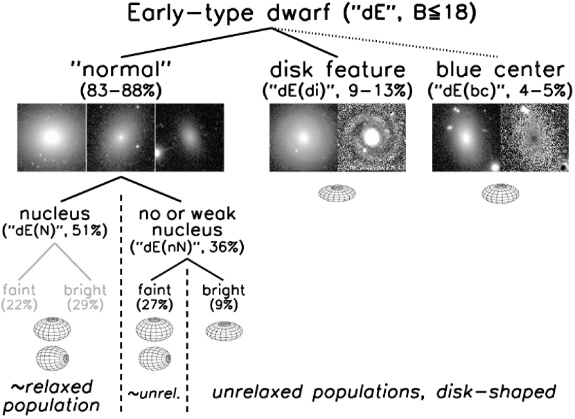
Figure 2.— The zoo of early-type dwarfs. Our subdivision is shown as tree scheme, along with a 3-D illustration of a typical intrinsic shape, using the median axial ratio from the intrinsic distributions shown in Fig. 3 (see Sect. 5.2). We also provide a statement about the inferred dynamical status of each subpopulation, as indicated by their clustering properties: “relaxed” and “unrelaxed” (see Sect. 5.3). The subdivision of dE(N)s into faint and bright samples is shown in grey color to reflect the fact that we find them to be not different in their properties (see Sect. 5). The branch of the dE(bc)s is shown as dotted line only, since these are not a morphological subclass (see text). The percentage of each subsample among our 413 Virgo cluster dEs is given in parentheses. For the dE(bc)s and dE(di)s the percentage ranges include corrections for the estimated number of objects missed by our detection techniques (see Papers I and II). Three sample images are shown for the normal dEs. For the dE(di)s, we show one sample image along with its unsharp mask revealing the spiral substructure. For the dE(bc)s, one sample image is shown along with its $g-i$ color map revealing the blue center (dark=blue). See text for further details.

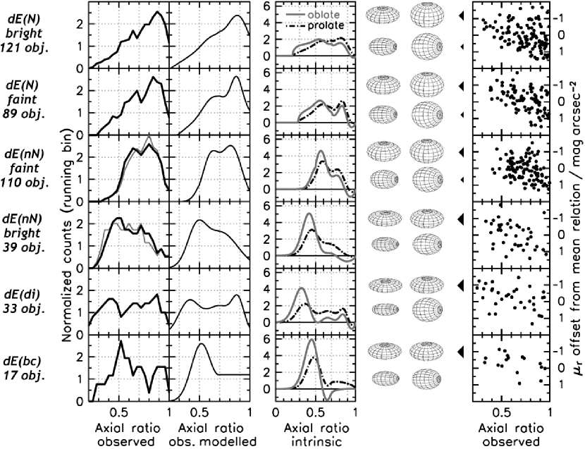
Figure 3.— Deduction of intrinsic shapes. In the leftmost column, the number of objects in each of our dE subsamples are given. In the second column, we show the distribution of projected axial ratios for each of our dE subsamples. The data are shown as running histogram with a bin width of 0.15, corresponding to one fifth of the range in axial ratio covered by our galaxies. Each curve is sampled in steps of 0.04 (one quarter of the bin width) and normalized to an area of 1. The observed distributions are approximated by analytic functions (see text), shown in the third column. From these, we derive intrinsic axial ratio distributions (fourth column), adopting purely oblate (grey solid line) and purely prolate (black dash-dotted line) shapes. For these distributions, we show in the fifth column 3-D illustrations of the galaxy shapes for the oblate (upper) and prolate (lower) case. For each distribution, we show the shape when using the 25th percentile axial ratio (left) and the 75th percentile axial ratio (right). In the rightmost column, we show for each dE subsample the surface brightness test (see text): we plot the surface brightness offset from the mean relation of $r$ band surface brightness and magnitude against axial ratio. Surface brightness is measured within $a=2a_{{\rm hl},r}$, since axial ratio is measured at the same semimajor axis. The mean relation of surface brightness and magnitude is obtained through a linear least squares fit with one 3$\sigma$-clipping. The arrows pointing from the surface brightness test diagrams towards the shape illustrations reflect whether the test implies oblate or prolate intrinsic shapes; see text for more details.

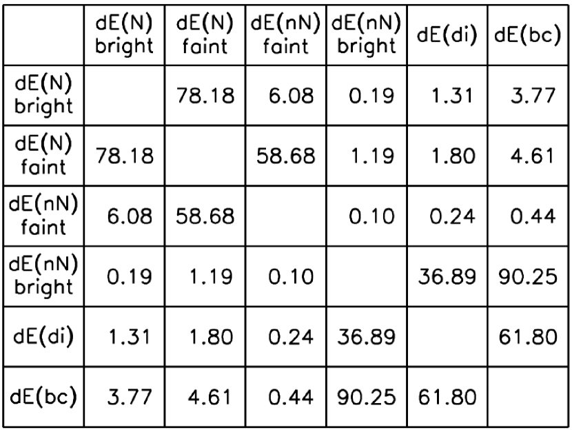
Figure 4.— K-S test results for the comparison of the axial ratio distributions of our dE subsamples. For each pair of distributions we give the probability in percent for the null hypothesis that the two distributions stem from the same underlying distribution function.

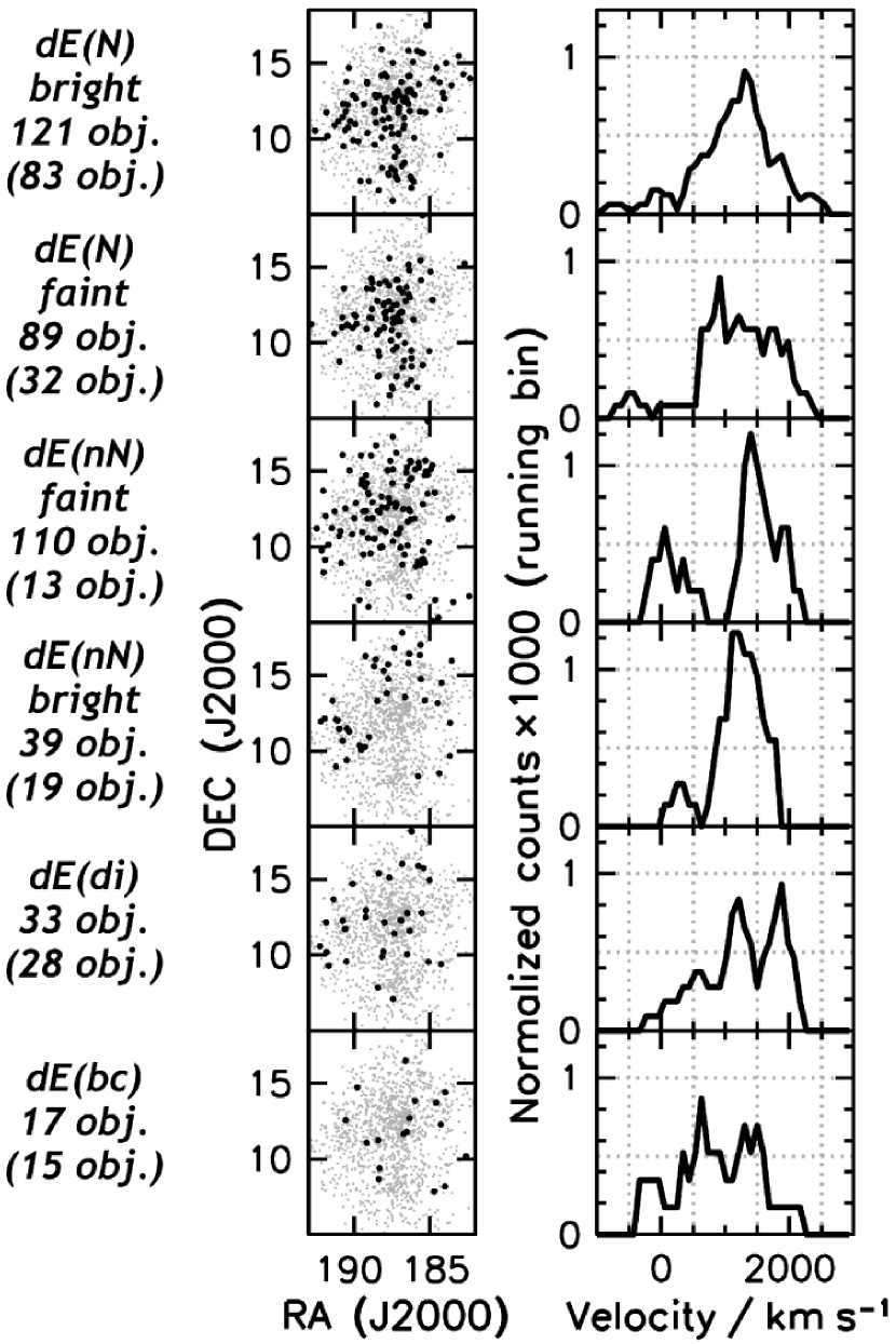
Figure 5.— Spatial and velocity distribution. In the left column, the number of objects in each of our dE subsamples are given. Numbers in parentheses apply to those dEs for which heliocentric velocities are available. The middle column shows the projected distribution of the dE subsamples (black dots) within the cluster. All Virgo cluster member galaxies are shown as small grey dots. The right column shows the velocity distributions of the dE subsamples. The data are shown as running histogram with a bin width of $384\,$km/s, corresponding to the semi-interquartile range of the total 193 velocities. Each curve is sampled in steps of $96\,$km/s (one quarter of the bin width) and normalized to an area of 1.

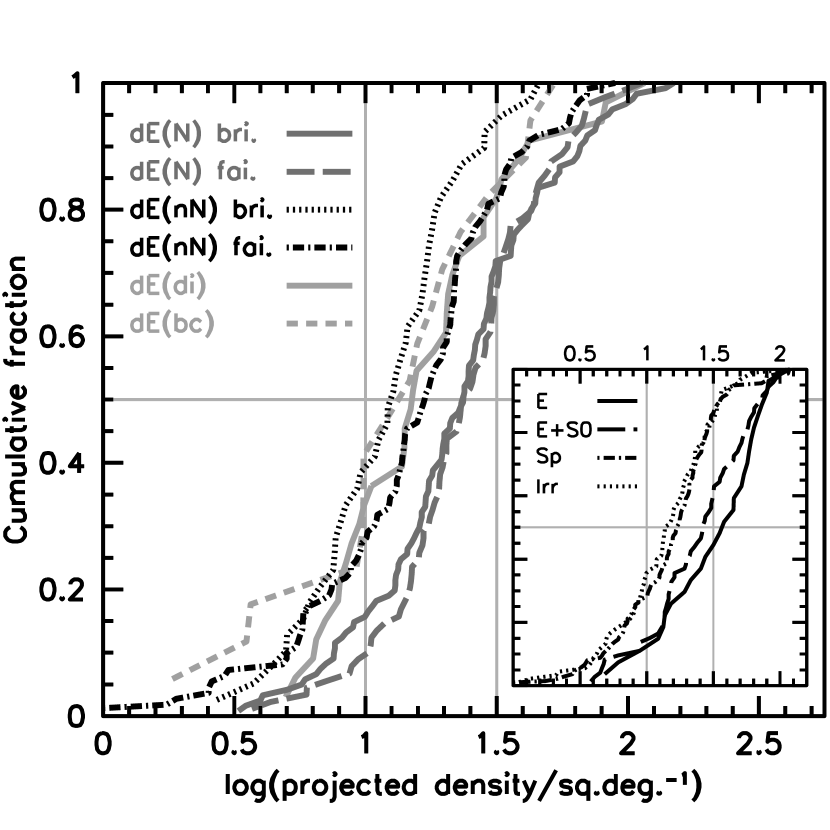
Figure 6.— Morphology vs. density. Cumulative distribution of local projected densities of our dE subsamples, and of Hubble types (inset). Following Dressler (1980) and Binggeli et al. (1987), we define a circular area around each galaxy that includes its ten nearest neighbours (independent of galaxy type), yielding a projected density (number of galaxies per square degree).

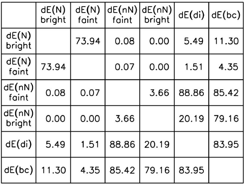
Figure 7.— K-S test results for the comparison of the distributions of our dE subsamples with respect to local projected density. For each pair of distributions we give the probability in percent for the null hypothesis that the two distributions stem from the same underlying distribution function.

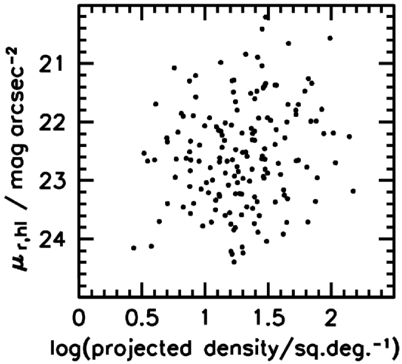
Figure 8.— Surface brightness vs. density. The mean surface brightness in $r$ within the half-light aperture is compared to local projected density for the combined sample of bright dE(N)s and dE(nN)s, in order to test for a possible classification bias as conjectured by Côté et al. (2006) (see text). No correlation is seen, ruling out such a bias.

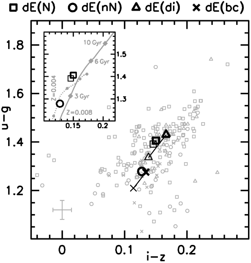
Figure 9.— Distribution in color space. Shown are the inner $u-g$ versus $i-z$ colors, measured within $a=0.5a_{{\rm hl},r}$, for all dEs brighter than the median $r$ brightness of our full sample, $m_{\mathrm{r}}=15.67$ mag, divided into the respective subsamples. Individual measurements are shown with small grey symbols (see the legend above the diagram). The median value of each subsample is shown as black symbol using thick lines. Black symbols drawn with thin lines represent the median values corrected for the effect of the color-magnitude-relation (see text); lines connect them to the corresponding uncorrected values. The correction is chosen to be zero for the dE(nN)s. The inset shows again the median values (corrected and uncorrected) of the dE(N)s and dE(nN)s, along with two model tracks from stellar population synthesis calculations (Bruzual & Charlot, 2003). Both tracks represent stellar populations formed through a single burst of star formation that exponentially decays with time ($\tau=0.5$ Gyr), using Padova 2000 isochrones and a Chabrier IMF. The grey solid line is for a metallicity $Z=0.008$; age steps are marked by the grey diamonds at 3 Gyr, 6 Gyr, and 10 Gyr. The grey dotted line is for $Z=0.004$, with age steps marked by the grey circles at 3 Gyr, 6 Gyr, 10 Gyr, and 14 Gyr; the latter is also the end of the track.

References

- Abraham et al. (1994) Abraham, R. G., Valdes, F., Yee, H. K. C., & van den Bergh, S. 1994, ApJ, 432, 75
- Adelman-McCarthy et al. (2006) Adelman-McCarthy, J. K., et al. 2006, ApJS, 162, 38
- Adelman-McCarthy et al. (2007) —. 2007, ApJS, submitted
- Aguerri et al. (2005) Aguerri, J. A. L., Iglesias-Páramo, J., Vílchez, J. M., Muñoz-Tuñón, C., & Sánchez-Janssen, R. 2005, AJ, 130, 475
- Arnaboldi et al. (2004) Arnaboldi, M., Gerhard, O., Aguerri, J. A. L., Freeman, K. C., Napolitano, N. R., Okamura, S., & Yasuda, N. 2004, ApJ, 614, L33
- Barazza et al. (2002) Barazza, F. D., Binggeli, B., & Jerjen, H. 2002, A&A, 391, 823
- Barazza et al. (2003) —. 2003, A&A, 407, 121
- Bertin & Arnouts (1996) Bertin, E. & Arnouts, S. 1996, A&AS, 117, 393
- Binggeli & Cameron (1991) Binggeli, B. & Cameron, L. M. 1991, A&A, 252, 27
- Binggeli & Popescu (1995) Binggeli, B. & Popescu, C. C. 1995, A&A, 298, 63
- Binggeli et al. (1993) Binggeli, B., Popescu, C. C., & Tammann, G. A. 1993, A&AS, 98, 275
- Binggeli et al. (1985) Binggeli, B., Sandage, A., & Tammann, G. A. 1985, AJ, 90, 1681
- Binggeli et al. (1987) Binggeli, B., Tammann, G. A., & Sandage, A. 1987, AJ, 94, 251
- Boselli & Gavazzi (2006) Boselli, A. & Gavazzi, G. 2006, PASP, 118, 517
- Bothun et al. (1986) Bothun, G. D., Mould, J. R., Caldwell, N., & MacGillivray, H. T. 1986, AJ, 92, 1007
- Bruzual & Charlot (2003) Bruzual, G. & Charlot, S. 2003, MNRAS, 344, 1000
- Buyle et al. (2005) Buyle, P., De Rijcke, S., Michielsen, D., Baes, M., & Dejonghe, H. 2005, MNRAS, 360, 853
- Conselice et al. (2000) Conselice, C. J., Bershady, M. A., & Jangren, A. 2000, ApJ, 529, 886
- Conselice et al. (2001) Conselice, C. J., Gallagher, III, J. S., & Wyse, R. F. G. 2001, ApJ, 559, 791
- Conselice et al. (2003) Conselice, C. J., O’Neil, K., Gallagher, J. S., & Wyse, R. F. G. 2003, ApJ, 591, 167
- Côté et al. (2006) Côté, P., et al. 2006, ApJS, 165, 57
- Davies & Phillipps (1988) Davies, J. I. & Phillipps, S. 1988, MNRAS, 233, 553
- De Rijcke et al. (2003) De Rijcke, S., Dejonghe, H., Zeilinger, W. W., & Hau, G. K. T. 2003, A&A, 400, 119
- Dressler (1980) Dressler, A. 1980, ApJ, 236, 351
- Drinkwater et al. (2001) Drinkwater, M. J., Gregg, M. D., Holman, B. A., & Brown, M. J. I. 2001, MNRAS, 326, 1076
- Fall & Frenk (1983) Fall, S. M. & Frenk, C. S. 1983, AJ, 88, 1626
- Ferguson & Sandage (1989) Ferguson, H. C. & Sandage, A. 1989, ApJ, 346, L53
- Ferrarese et al. (2000) Ferrarese, L., et al. 2000, ApJ, 529, 745
- Geha et al. (2003) Geha, M., Guhathakurta, P., & van der Marel, R. P. 2003, AJ, 126, 1794
- Graham et al. (2003) Graham, A. W., Jerjen, H., & Guzmán, R. 2003, AJ, 126, 1787
- Grant et al. (2005) Grant, N. I., Kuipers, J. A., & Phillipps, S. 2005, MNRAS, 363, 1019
- Grebel (1997) Grebel, E. K. 1997, in Reviews in Modern Astronomy 10, ed. R. E. Schielicke, 29
- Grebel et al. (2003) Grebel, E. K., Gallagher, J. S., & Harbeck, D. 2003, AJ, 125, 1926
- Gunn et al. (1998) Gunn, J. E., et al. 1998, AJ, 116, 3040
- Gunn & Gott (1972) Gunn, J. E. & Gott, J. R. I. 1972, ApJ, 176, 1
- Jerjen & Binggeli (2005) Jerjen, H. & Binggeli, B., eds. 2005, Near-field cosmology with dwarf elliptical galaxies, IAU Colloq. 198 (Cambridge: CUP)
- Jerjen et al. (2000) Jerjen, H., Kalnajs, A., & Binggeli, B. 2000, A&A, 358, 845
- Joye & Mandel (2003) Joye, W. A. & Mandel, E. 2003, in ASP Conf. Ser. 295, Astronomical Data Analysis Software and Systems XII, ed. H. E. Payne, R. I. Jedrzejewski, and R. N. Hook (San Francisco: ASP), 489
- Lisker et al. (2006b) Lisker, T., Glatt, K., Westera, P., & Grebel, E. K. 2006b, AJ, 132, 2432, Paper II
- Lisker et al. (2005) Lisker, T., Grebel, E. K., & Binggeli, B. 2005, in IAU Colloq. 198: Near-field cosmology with dwarf elliptical galaxies, ed. H. Jerjen & B. Binggeli (Cambridge: CUP), 311
- Lisker et al. (2006a) Lisker, T., Grebel, E. K., & Binggeli, B. 2006a, AJ, 132, 497, Paper I
- Lotz et al. (2004b) Lotz, J. M., Miller, B. W., & Ferguson, H. C. 2004b, ApJ, 613, 262
- Lotz et al. (2004a) Lotz, J. M., Primack, J., & Madau, P. 2004a, AJ, 128, 163
- Marchant & Olson (1979) Marchant, A. B. & Olson, D. W. 1979, ApJ, 230, L157
- Mastropietro et al. (2005) Mastropietro, C., Moore, B., Mayer, L., Debattista, V. P., Piffaretti, R., & Stadel, J. 2005, MNRAS, 364, 607
- Moore et al. (1996) Moore, B., Katz, N., Lake, G., Dressler, A., & Oemler, A. 1996, Nature, 379, 613
- Moore et al. (1998) Moore, B., Lake, G., & Katz, N. 1998, ApJ, 495, 139
- Oh & Lin (2000) Oh, K. S. & Lin, D. N. C. 2000, ApJ, 543, 620
- Oke & Gunn (1983) Oke, J. B. & Gunn, J. E. 1983, ApJ, 266, 713
- Papaderos et al. (1996) Papaderos, P., Loose, H.-H., Fricke, K. J., & Thuan, T. X. 1996, A&A, 314, 59
- Petrosian (1976) Petrosian, V. 1976, ApJ, 209, L1
- Pier et al. (2003) Pier, J. R., Munn, J. A., Hindsley, R. B., Hennessy, G. S., Kent, S. M., Lupton, R. H., & Ivezić, Ž. 2003, AJ, 125, 1559
- Rakos & Schombert (2004) Rakos, K. & Schombert, J. 2004, AJ, 127, 1502
- Richer et al. (1998) Richer, M., McCall, M. L., & Stasinska, G. 1998, A&A, 340, 67
- Richstone (1979) Richstone, D. O. 1979, ApJ, 234, 825
- Ryden & Terndrup (1994) Ryden, B. S. & Terndrup, D. M. 1994, ApJ, 425, 43
- Sandage & Binggeli (1984) Sandage, A. & Binggeli, B. 1984, AJ, 89, 919
- Schlegel et al. (1998) Schlegel, D. J., Finkbeiner, D. P., & Davis, M. 1998, ApJ, 500, 525
- Stoughton et al. (2002) Stoughton, C., et al. 2002, AJ, 123, 485
- Thuan (1985) Thuan, T. X. 1985, ApJ, 299, 881
- Tody (1993) Tody, D. 1993, in ASP Conf. Ser. 52: Astronomical Data Analysis Software and Systems II, 173
- Tully & Shaya (1984) Tully, R. B. & Shaya, E. J. 1984, ApJ, 281, 31
- van den Bergh (1986) van den Bergh, S. 1986, AJ, 91, 271
- van Zee et al. (2004) van Zee, L., Skillman, E. D., & Haynes, M. P. 2004, AJ, 128, 121