Ten–year optical monitoring of PKS 0735+178: historical comparison, multiband behaviour and variability timescales

Abstract

Aims. New data and results on the optical behaviour of the prominent blazar PKS 0735+178 (also know as OI 158, S3 0735+17, DA 237, 1ES 0735+178, 3EG J0737+1721) are presented, through the most continuous $BVRI$ data available in the period 1994-2004 (about 500 nights of observations). In addition, the whole historical light curve, and a new photometric calibration of comparison stars in the field of this source are reported.

Methods. Several methods for timeseries analysis of sparse data sets are developed, adapted and applied to the reconstructed historical light curve and to each observing season of our unpublished optical database on PKS 0735+178. Optical spectral indexes are calculated from the multi-band observations and studied on long-term (years) durations as well. For the first time in this source, variability modes, characteristic timescales and the signal power spectrum are explored and identified over 3 decades in time with a sufficient statistics. The novel investigation of mid-term optical scales (days, weeks), could be also applied and compared to blazar gamma-ray light curves that will be provided, on the same timescales, by the forthcoming GLAST observatory.

Results. In the last 10 years the optical emission of PKS 0735+178 exhibited a rather achromatic behaviour and a variability mode resembling the shot-noise. The source was in a intermediate or low brightness level, showing a mild flaring activity and a superimposition/succession of rapid and slower flares, without extraordinary and isolated outbursts but, at any rate, characterized by one major active phase in 2001. Several mid-term scales of variability were found, the more common falling into duration intervals of about 27-28 days, 50-56 days and 76-79 days. Rapid variability in the historical light curve appears to be modulated by a general, slower and rather oscillating temporal trend, where typical amplitudes of about 4.5, 8.5 and 11-13 years can be identified. This spectral and temporal analysis, accompanying our data publication, suggests the occurrence of distinctive signatures at mid-term durations that can likely be of transitory nature. On the other hand the possible pseudo-cyclical or multi-component modulations at long times could be more stable, recurrent and correlated to the bimodal radio flux behaviour and the twisted radio structure observed by several years in this blazar.

1 Introduction

The rapid and violent optical variability is one of the defining properties of blazars, and variability studies are important in understanding the physics of AGN in general. Characteristic timescales, fluctuations modes, flares shapes and amplitudes, duty cycles and spectral changes, correlations and temporal lags between variations in different spectral bands, provide crucial information on the nature, structure and location of the emission components and on their interdependencies. In particular the so called low/intermediate–frequency peaked BL Lac objects (LBL/IBL), have the peak of the synchrotron emission around infrared and optical wavelengths and commonly show large-amplitude flares characterized by prominent flux variations in a wide range of temporal scales. The rapid optical variations of LBL and IBL are also systematically larger and with shorter duty cycles than those of the high energy peaked BL Lac objects (HBL). Hence a multi-band, possibly well sampled and extended optical monitoring is an important and subsidiary element of the standard multiwavelength (MW) analysis. MW observing campaigns provide, more or less, short snapshots of the targets, lacking of information about their mid/long-term evolution. Even if the optical band has a narrow spectral extension, it can yield useful information about the synchrotron emission peak and possible disk/host-galaxy contributions. Moreover long-term (historical) records of blazar variability are available at optical wavelengths for several bright objects, although data collected in the past are rather sparse. Small–size and dedicated (possibly automatic) telescopes, in conjunction with international consortiums, have recently increased the amount of photometric data, sometimes with a fair continuous sampling during specific observing campaigns.

In this paper we present more than 10 years (Feb.1993–Feb.2004) monitoring data about the blazar PKS 0735+178 (1332 photometric points in four $BVRI$ Johnson-Cousins filters, obtained during about 500 observing nights). Our effort represents the best optical monitoring available for this object regarding to continuous and long–term coverage. This optical programme allowed to study colours and the continuum spectrum (mainly in $VRI$ bands) and, for the first time, enabled to study mid-term scales (days, weeks), over an extended data set. These timescales were almost unexplored in blazars due to the irregular/poor sampling and the low statistics in the optical regime. Time series analysis accompanying our data publication, is performed for both our observations and the historical light curve (1906-2004), while a new photometric calibration of comparison stars in the field of the source is also reported, as useful reference for future optical observations and monitoring. In the historical light curve there are obvious differences in data quality, accuracy and sampling over time, that can yield biases, noise, spurious and fakes signatures. However we remark that the last 33 years portion (1970-2004) of the historical light curve holds a sufficiently regular sampling to allow meaningful statistical results on long-term intervals too. Data binning when needed, the employment and comparison of 7 different temporal analysis methods suitable for unevenly sampled data set, and the calculation of the power spectrum given by the gaps, secure us to have determined and reported only real and intrinsic time signatures. We note finally that the main aim of our paper was to investigate the variability behaviour on such intermediate scales through our 10-year observations. Data published in this work were obtained by 4 optical observatories: the Perugia University Observatory (Italy), the INAF Torino Observatory (Italy), the Tuorla Observatory (Finland), and the Sabadell Observatory (Spain). Perugia, Torino and Sabadell data on PKS 0735+178 are unpublished, while part of the Tuorla data were already published in Katajainen et al. (2000). Optical data from Qian & Tao (2004) have been also added to improve a few the sampling.

The paper is organized as follows: in Sect. 2 we review briefly the optical knowledge about PKS 0735+178, while in Sect. 3 we mention the observing and data reduction techniques. A new photometric calibration of comparison stars in the field of the source is presented in Sect. 4, and the $BVRI$ light curves collected during our monitoring are showed in Sect. 5. The reconstructed historical light curve is described in Sect. 6 while in Sect. 7 the analysis of the multi–band behaviour is reported computing the optical spectral indexes. A joint temporal analysis of our data and the historical light curve is performed in Sect. 8, and summary and conclusions are outlined in Sect. 9.

2 Optical properties of PKS 0735+178

The radio object PKS 0735+178, belonging to the Parkes catalog (other most used names are: PKS 0735+17, S3 0735+17, OI 158, DA 237, VRO 17.07.02, PG 0735+17, RGB J0738+177, 1Jy 0735+17, RX J0738.1+1742, 3EG J0737+1721) was identified with an optical point source by Blake (1970). Afterwards it was classified as a classical BL Lac object in Carswell et al. (1974). This source is optically bright, highly variable, and both radio (Kühr et al., 1981) and X-ray selected (Elvis et al., 1992). PKS 0735+178 has been extensively studied in the radio regime. The radio flux appear to vary quite slowly with some outbursts (Bååth & Zhang, 1991; Teräsranta et al., 1992; Aller et al., 1999; Teräsranta et al., 2004), but there is not any evidence of a radio-optical correlation (Clements et al., 1995; Hanski, Takalo, & Valtaoja, 2002) or periodicity (Ciaramella et al., 2004). Early radio observations of PKS 0735+178 showed a peculiar spectrum soon interpreted as the superposition of incoherent synchrotron radiation emitted by distinct and homogeneous radio components, conspiring to add up to an overall very flat shape (the source was indeed nicknamed as the “Cosmic Conspiracy” Marscher, 1977, 1980; Cotton et al., 1980). Several moving components and an unusual, complex morphology characterized by a twisted jet were observed in VLBA/VLBI radio imaging (see, e.g. Perlman & Stocke, 1994; Gabuzda et al., 1994; Gabuzda, Gómez, & Agudo, 2001; Gómez et al., 2001; Homan et al., 2002; Ojha et al., 2004; Kellermann et al., 2004). PKS 0735+178 has one of the most bent radio jets among AGN observed at milliarcsecond (mas) scales. A bimodal scenario in which periods of enhanced activity with ejection of superluminal components are followed by epochs of low activity with a highly twisted jet geometry was suggested (Gómez et al., 2001; Agudo et al., 2006). PKS 0735+178 is also a X-ray and gamma-ray (EGRET, 3EG J0737+1721) emitting blazar (Kubo et al., 1998; Hartman et al., 1999, see, e.g. ). The spectral energy distribution (SED) evinced PKS 0735+178 as a low or intermediate–energy peaked BL Lac object (LBL/IBL), where the IR-UV synchrotron continuum dominates the total observed power. The very low X-ray variability with respect to the high optical-IR variations, supported the idea that X-rays are produced by inverse Compton mechanism in some mas radio components (Bregman et al., 1984; Madejski & Schwartz, 1988). The $\gamma$-ray flux of this blazar appeared likewise no strongly variable (Nolan et al., 2003).

The optical spectrum of PKS 0735+178 shows an absorption line due to an intervening system at 3980 $\mathrm{\AA}$ that, if identified with Mg-II, provides a lower redshift limit of $z>0.424$ (Carswell et al., 1974; Burbidge & Hewitt, 1987; Falomo & Ulrich, 2000; Rector & Stocke, 2001). A strong Lyman-alpha absorption line has also been detected by the IUE satellite at the same redshift (Bregman, Glassgold, & Huggins, 1981). This absorption was not identified in deep optical imaging, even if a very faint emission was detected about 3.0-3.5” NE/E (projected distance 22-25 kpc at $z=0.424$) from the object (Falomo & Ulrich, 2000; Pursimo et al., 2002). The host galaxy of PKS 0735+178 remains unresolved in optical imaging (Scarpa et al., 2000; Falomo & Ulrich, 2000; Pursimo et al., 2002), but the source has two well resolved companion galaxies. The galaxy at 7” NW, declared distorted by interaction with PKS 0735+178 (Hutchings, Johnson, & Pyke, 1988), does not show marks of interaction in more recent and higher resolution images, and a redshift of $z=0.645$ was obtained for it (Stickel, Fried, & Kuehr, 1993; Scarpa et al., 2000; Falomo & Ulrich, 2000). In addition a brighter galaxy located at 8.1” SE cannot be the absorber due to the great projected distance from our blazar. A third, very faint, elongated structure at 3-3.5” NE was detected as well (Pursimo et al., 1999; Falomo & Ulrich, 2000), and this could be related to the intervening absorption at $z=0.424$. The lower limit for the redshift $z>0.5$ obtained assuming typical properties for the host (Falomo & Ulrich, 2000) is consistent with the limit derived from intervening absorption.

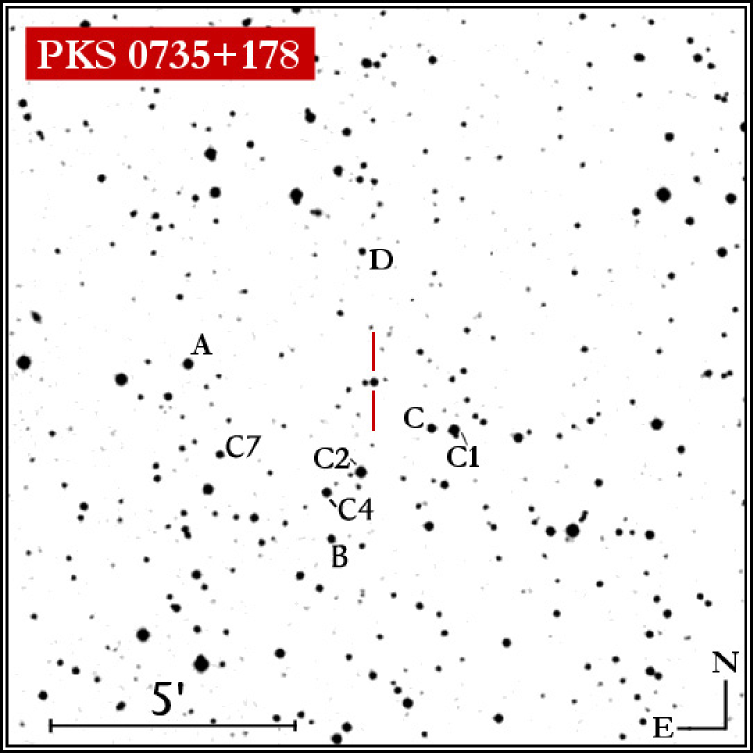
Figure 1: Finding chart with the optical comparison stars identified in a field of 15’$\times$15’ centered on PKS 0735+178 (within the double bar). The field is elaborated from a frame of the Digitized Sky Survey. The new photometric $VRI$ calibration of the stars C1, C, D, C2, C4, C7, and A is reported in Table 1. A, C, and D stars belong also to the photometric sequence calibrated by Smith et al. (1985), to the photometric sequence published in Wing (1973, here with a B sequence too), and the sequence appeared in Veron & Veron (1975, A and D stars only). Stars C2, C4, C7 belong also to the photometric sequence calibrated by McGimsey et al. (1976, named there 1,2,3), while for the C1 star the calibration is totally new.

When combined with our data the historical optical curve of PKS 0735+178, starting from JD 2417233, i.e. Jan. 22, 1906 (Fan et al., 1997), spans almost 100 years. Optical variations are often of larger amplitudes than the infrared one (Fan & Lin, 2000). Correlations between the spectral index and the optical brightness were observed (Sitko & Sitko, 1991; Lin & Fan, 1998), alongside a spectral flattening (blueing) with the source brightening (Brown et al., 1989; Lin & Fan, 1998). On the other hand this type of correlation appear to be weak (Gu et al., 2006) or opposite (i.e. spectral steepening, reddening; Ghosh et al., 2000) in other multiband observations. The largest optical variations registered are on the order of 3-4 mag (Pollock et al., 1979; Fan et al., 1997) at long (years) ranges. Some intra-day (IDV) and inter-day variations until 0.5 mag were reported in the optical history of this blazar (Xie et al., 1992; Fan et al., 1997; Massaro et al., 1995; Zhang et al., 2004). Over the period 1995-1997, the optical IDV and microvariations were rare and with a small amplitude (Bai et al., 1999), while no clear evidence was found in more recent observations (Sagar et al., 2004). Several possible recurrent and pure periodical components were claimed, with values of 1.2, 4.8 years (Smith, Leacock, & Webb, 1988; Webb et al., 1988; Smith & Nair, 1995); 14.2, 28.7 years (Fan et al., 1997); 8.6, 13.8, 19.8, 37.8 years (Qian & Tao, 2004), even if we remark that such scales are derived by different data sets and different epochs. The long–term analysis performed with the Jurkevich’s method on a more complete data set (Fan et al., 1997; Qian & Tao, 2004) postulated a main periodical component of about 13.8-14.2 years, but our temporal analysis (Section8) suggest other and shorter long-term signatures.

PKS 0735+178 has also a relatively high degree of optical polarization showing very different levels covering the whole range from about 1% up to 30% (see, e.g. Mead et al., 1990; Takalo, 1991; Takalo et al., 1992; Valtaoja et al., 1991, 1993; Tommasi et al., 2001). Only a modest variability of this optical polarization was observed on inter/intra night durations, that was interpreted as owed to substructures of different polarization and variable intensity in the jet. A preferred polarization level over few years (Tommasi et al., 2001) could indicate quiescence and stability in the underlying jet structure.

Table 1: A new optical photometric calibrations for field of PKS 0735+178, with $VR_{c}I_{c}$ Johnson-Cousins sequences of comparison stars C1, C, D, C2, C4, C7 and A (see Fig. 1). Data are obtained at the Perugia University Observatory and are adopted in this work. The previous available comparison sequences were published in Smith et al. (1985); Wing (1973); Veron & Veron (1975); McGimsey et al. (1976); Smith et al. (1985). Magnitudes of common stars are roughly in agreement within the uncertainties. The $VR_{c}I_{c}$ sequence reported in this table, joint with the $U,B$ values reported by Smith et al. (1985), is suggested for future optical observations and monitoring.

PHOTOMETRIC SEQUENCES FOR PKS 0735+178 COMPARISON STARS

Star	R.A.	Dec.	$V$	$R_{c}$	$I_{c}$
	(J2000.0)	(J2000.0)	[mag]	[mag]	[mag]
C1………………………………….	07 38 00.5	+17 41 19.9	13.26 $\pm$ 0.04	12.89 $\pm$ 0.04	12.57 $\pm$ 0.04
C……………………………………	07 38 02.4	+17 41 22.2	14.45 $\pm$ 0.04	13.85 $\pm$ 0.04	13.32 $\pm$ 0.04
D……………………………………	07 38 08.3	+17 44 59.7	15.90 $\pm$ 0.05	15.49 $\pm$ 0.05	15.12 $\pm$ 0.06
C2………………………………….	07 38 08.5	+17 40 29.2	13.31 $\pm$ 0.04	12.79 $\pm$ 0.04	12.32 $\pm$ 0.04
C4………………………………….	07 38 11.6	+17 40 04.4	14.17 $\pm$ 0.05	13.80 $\pm$ 0.04	13.48 $\pm$ 0.04
C7………………………………….	07 38 20.7	+17 40 51.2	15.01 $\pm$ 0.06	14.70 $\pm$ 0.06	14.37 $\pm$ 0.05
A……………………………………	07 38 23.4	+17 42 43.0	13.40 $\pm$ 0.05	13.10 $\pm$ 0.05	12.82 $\pm$ 0.05

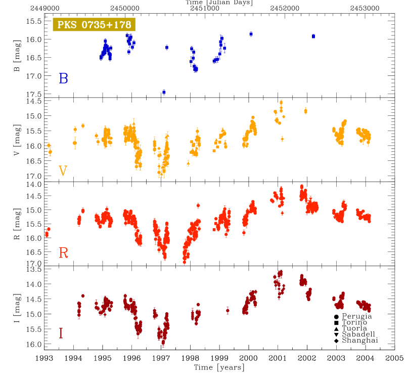
Figure 2: $BVRI$ magnitude light curves of PKS 0735+178 from 1993 to beginning of 2004. Data cames from our 10-year observing monitoring. Published observations from Shanghai Observatory (Qian & Tao, 2004) are added in order to improve the sampling. Data sets of different observatories are in agreement within the uncertainties.

3 Observations and data reduction

Photometric observations were carried out with four telescopes. The Newtonian f/5, 0.4 m, Automatic Imaging Telescope (AIT) of the Perugia University Observatory, Italy (451 meters above sea level, a.s.l.), a robotic telescope equipped with a $192\times 165$ pixels CCD array, thermoelectrically cooled with Peltier elements (Tosti, Pascolini, & Fiorucci, 1996). The REOSC f/10, 1.05 m, astrometric reflector of the Torino Observatory, Italy (622 meters a.s.l.), mounting a $1242\times 1152$ pixel CCD array, cooled with liquid nitrogen and giving an image scale of $0.467^{\prime\prime}$ per pixel. The Dall-Kirkham f/8.45, 1.03 m reflector of the Turku University Tuorla Observatory, Finland (60 meter a.s.l.), equipped with a $1530\times 1020$ pixel CCD camera, thermoelectrically cooled. The Newtonian 0.5m telescope of the Sabadell Observatory, Spain used in two interchangeable configurations (Newton at f/4, and Cassegrain-Relay at f/15), and equipped with a $512\times 512$ FLI CM-9 CCD array. The Perugia and Torino telescopes were provided with standard $BV$ (Johnson) and $R_{c}I_{c}$ (Cousins) filters (Bessell, 1979; Fiorucci & Munari, 2003; Bessell, 2005). The Tuorla 1m telescope, and the Sabadell telescope were equipped with V and $R_{c}$ filters.

All the observatories took CCD frames and performed a first automatic data reduction using standard methods, to correct each raw image (for dark and bias background signals where needed) and to flat fielding, to recognize the field stars, and to derive instrumental magnitudes via aperture photometry (Perugia and Tuorla) or circular Gaussian fitting (Torino). The single frames are then inspected to evaluate the quality of the image, the reliability of the data, and to search for spurious interferences. Comparison among data obtained with these different telescopes on the same night reveals a good agreement, and no detectable offset is found. The matching with data taken in simultaneous epochs at Shanghai Observatory (Qian & Tao, 2004) showed a good agreement too (see Fig. 3). The precision level in the light curve of PKS 0735 assembled in this way is enough for a variability analysis performed on intermediate and long–term timescales. Moreover the time series analysis of shorter timescales ($<200$ days) is performed in each single observing season using $R$-band data, that were mainly obtained by 1 telescope (see Tab. 2).

4 Comparison stars photometry

Calculation of the source magnitude is easily obtained by differential photometry with respect to comparison stars in the same field of the object. The discussion of the adopted comparison star sequence is crucial for analysis of optical data obtained during blazar monitoring observations, as the photometric sequence affects data quality and reliability. In order to obtain a dependable photometric sequence for PKS 0735+178, we selected a set of non–variable stars with brightness comparable to the object and different colours (see the finding chart in Fig. 1). Photometric calibrations of these stars were derived from 13 optimal photometric nights between 1994 and 1996 at the Perugia University Observatory using Landolt standards. The stability of the sequence for the stars C1, C, D, C2, C4, was well tested and verified during data reduction of the overall database (for stars A and C7 there are less measurements because of the small FOV of the instrument). Our new photometric sequence is presented in Table 1, showing the $V$ (Johnson), and $R_{c},I_{c}$ (Cousins) photometric values. Previous calibrations of this star–field were performedin in Wing (1973); Veron & Veron (1975); McGimsey et al. (1976); Smith et al. (1985). In particular the determinations of McGimsey et al. (1976) are photoelectric in the $UBV$ Johnson system, thus well similar to our calibrations in $B,V$ bands using a CCD detector. Discrepancies are small if the specifications of Bessell (1990) are respected and determined (Fiorucci & Munari, 2003).

This new photometric calibration of the PKS 0735+178 field, (suitable also for telescopes with small FOV), is slightly more extended and accurate with respect to the past calibrations. Table 1 reports the $V,R_{c}$, $I_{c}$ values for seven comparison stars, while the sequence for the star denoted with C1 is completely new. In each photometric night standard Landolt stars were observed at different airmasses, and the calibration line as a function of the airmass was constructed (neglecting the colour corrections being always smaller than the instrumental errors). The standard magnitudes of such stars were derived (with error equal to the quadrature sum of the linear regression error and the instrumental error on the single star). The typical error for each night and each star is between 0.03 and 0.1 mag (depending on the luminosity of the star and the atmospheric conditions). Data shown in Table 1 are the result of weighted averages on the values of each night (weight equal to $1/\sigma^{2}$), whereas the error estimation is equal to the standard deviation weighted on the averages. This uncertain is higher than the standard deviation on each single night, because of some systematic errors different on each night. We chose to report a reliable calibration with reliable errors in Table 1 with respect to more accurate but more doubtful smoothed values. Colour transformations to comparison stars were not applied, because from the analysis of Landolt stars it was not possible to separate this effect from the instrumental statistical errors given mainly by the effective limits of the Perugia instrument and site. Then again the photometric system of the Perugia telescope was developed to follow at best the standard Johnson-Cousins system. Finally we note that some of the stars listed in Table 1 are quite red ($V-I$ index ranges from +0.58 to +1.13 mag, suggesting that they have spectral types F, G, possibly K), but these colour indexes are similar to the colour indexes of PKS 0735+178 (average $V-I=+0.95\pm 0.1$, average $B-R=+0.91\pm 0.09$) hence colour effects are correspondent, and $B$-band data were obtained only with the larger 1m Torino telescope. A detailed description of the observing and data reduction procedures, filter system, software adopted in the calibrations, and comparison with other works can be found in Fiorucci, Tosti, & Rizzi (1998); Fiorucci & Tosti (1996).

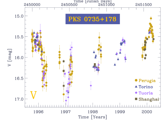
Figure 3: A portion of the V-mag light curve where is possible to see in more detail data from the different observatories.

Table 2: The number of photometric $BVRI$ data points of PKS 0735+178 obtained by each observatory in the period 1993-2004 and published in this paper. In the bottom panel a summary of the basic information and statistics about our data in each band.

DATA POINTS PER OBSERVATORY

Obs.	$B$	$V$	$R$	$I$	Tot.	Period
Perugia	0	226	490	281	997	Feb1993-Feb2004
Torino	75	38	150	0	263	Dec1994-Apr2002
Tuorla	0	55	0	0	55	Oct1995-Feb2001
Sabadell	0	0	17	0	17	Dec2001-Feb2004
Shanghai	0	115	52	138	305	Jan1995-Dec2001
Total	75	434	709	419	1637

  
  
1993-2004 DATA STATISTICS $B$ $V$ $R$ $I$ Total data points 75 434 709 419 Start date [JD-2449000] 698 45 21 420 End date [JD-2449000] 3354 4053 4053 4053 Total period $N_{tot}$ [days] 2657 4001 4032 3633 Nights with data $N_{on}$ 52 297 459 259 $N_{on}/N_{tot}$ fraction 0.019 0.074 0.171 0.071 Mean num. points $\times$ night 1.44 1.46 1.51 1.62 Total mean gap $\Delta t$ [days] 35.9 9.3 5.8 8.7 Longest gap [days] 780 352 375 356 Average brightness [mag] 16.319 15.760 15.301 14.693 Max brightness [mag] 15.863 14.544 14.16 13.59 Min brightness [mag] 17.453 16.94 16.87 15.97 Variab. range $\Delta m$ [mag] 1.59 2.39 2.71 2.38 Absorption coeff.^† [mag] 0.152 0.117 0.094 0.068 Data standard deviation 0.256 0.368 0.515 0.453 Data skewness 1.23 0.386 0.329 0.155 Data kurtosis 3.791 1.087 0.019 0.400 Max flux [mJy] $2.21$ $6.1$ $7.3$ $9.9$ Min flux [mJy] $0.51$ $0.67$ $0.60$ $1.1$

• Values for the galactic extinction by NED database (Schlegel, Finkbeiner, & Davis, 1998).

5 Optical light curves from 1993 to 2004

We monitored the BL Lac object PKS 0735+178 in the four $B,V,R_{c},I_{c}$ optical bands for more than 10 years, from February 2, 1993 to February 17, 2004 (JD=2449021–2453053). A total of 1332 $BVRI$ reduced and validated photometric points were obtained over a period of 4032 days (see Fig. 2). In order to obtain a more complete light curve, data from the Shanghai Observatory (Jan.1995-Dec.2001) are added Qian & Tao (2004). In the best sampled band (the $R$–band, analyzed in detail in Sect.8), 709 photometric points were collected over 12 observing seasons (see Tab.2 and Tab.3) with 459 nights in total having at least one $R$ data point. The last and best sampled 10 observing seasons (from the III to the XII, i.e. from October 1994 to February 2004) have a duration spanning from 144 to 203 days Tab.3), an average number of data points per night equal to 1.5, an average empty gap between subsequent observations of 3 days, and an average coverage of nights with data respect to each season duration of about 27%. Practically speaking such numbers mean that data are not clustered or bunched, and that an enough regular monitoring was performed (when permitted by atmospheric/technical conditions). The priority of our observing programme during these years was to perform a constant and possibly uniform optical monitoring. Consequently, for the first time in PKS 0735+178, this allowed to obtain data suitable for a deep and detailed statistical analysis on days/weeks timescales. The majority of such $R$–filter observations were obtained by only two telescopes (over the $69\%$ obtained by the Perugia telescope, and a further 21% by the Torino telescope) having known inter–instrumental offsets below 0.1 mag in this band (e.g. Villata et al., 2002; Böttcher et al., 2005). Three examples of such R-band seasonal light curves with the accompanying time series analysis functions are reported in Fig.10, Fig.11 and Fig.12.

A direct visual inspection of our 10-year multiband light curve (Fig. 2), show an average optical brightness placed at a mid or low levels, displaying rapid variability with a moderate flaring but no extraordinary big/isolated outburst ($R>14$ in the whole data set). Luminosity drops/increasing of about 2 magnitudes were common on time intervals smaller than half year. From the end of 1997, a slow increase of the average brightness was clearly detected (e.g. the $R$-band magnitude never dropped to values higher than 16 from beginning of 1998), while in 2001 a clear brightening phase can be well identified. This moderate-outburst phase can be considered comparable to the other outbursts seen in the optical history of PKS 0735+178 (see, Sec. 6).

6 The historical light curve

The optical history of PKS 0735+178 together with our data (Fig. 4) extends over almost one century (from Jan 22, 1906, JD 2417233, to Feb 17, 2004, JD 2453053).

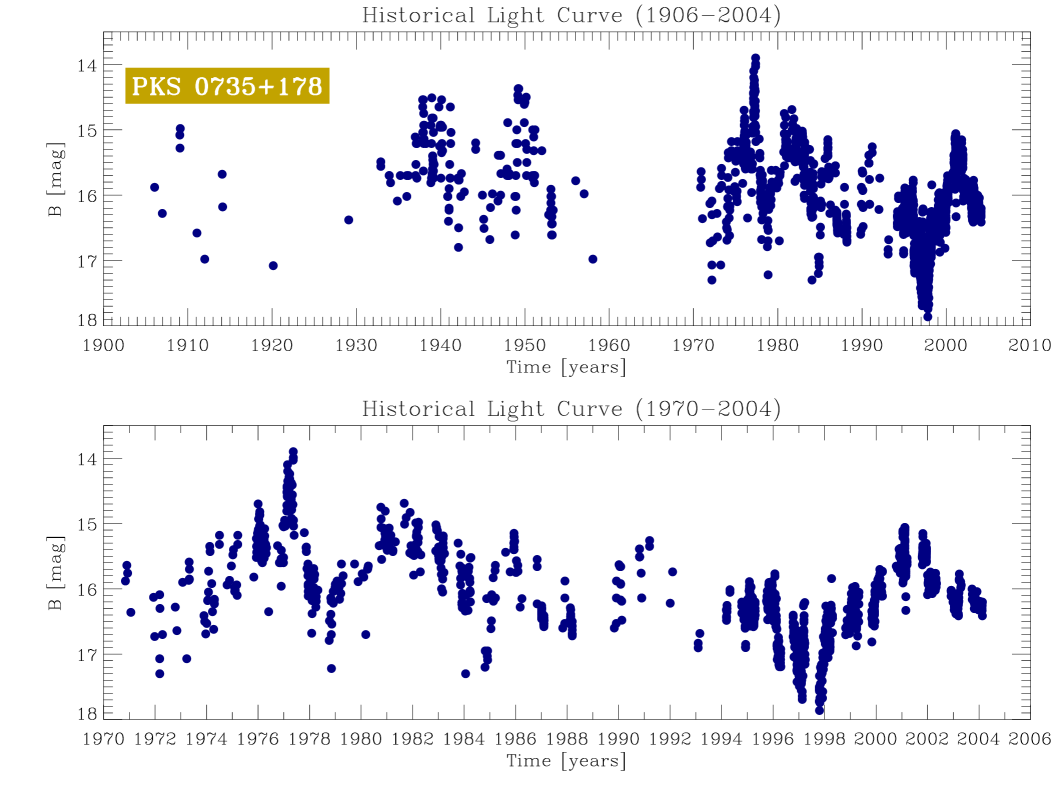
Figure 4: The historical optical light curve of PKS 0735+178 in $B$ band reconstructed by published data (data points mainly from the compilation of Qian & Tao, 2004, with more few data from other literature) and adding our original $B$ and $R$-derived data (see text). Error bars are not represented for clarity. The total historical time series obtained in this way is composed of 1725 final data points. At least five main outbursts followed by a general humped and rather oscillatory long-term trend can be visually recognized. This behaviour is identifiable better in the 1970-2004 portion (lower panel), thanks to a higher sampling (lower panel).

The older points in the light curve were obtained using plates (mainly from the Landessternwarte Heidelberg-Königstuhl Observatory, Germany, and the Rosemary Hill Observatory, Florida, USA Zekl et al., 1981; Webb et al., 1988), from which a photographic magnitude $m_{pg}$ can be extracted and converted in the photometric $B$ magnitude following a semi–empirical correction (see, e.g. Lu, 1972; Kidger, 1989). More recent data have been obtained directly with photoelectric or CCD instruments. The historical data collection was taken directly from (Qian & Tao, 2004) with few additions and appending our original and derived $B$-magnitudes (the derived $B$-band data are estimated from our best sampled $R$-mag data after 1993, using a constant colour index with value equal to previous works $B-R=0.993$, Fan et al., 1997; Qian & Tao, 2004). In general a prudential error estimation (taking into account different offsets, different data quality, systematic errors and instrumental dispersion), needs to be figured out, before to use heterogeneous historical optical light curves for a quantitative analysis. In this specific case the further errors introduced by using a constant conversion index from the $R$ and $B$ band has also to be counted on. This estimation is difficult without all the original data sets (plates, frames, etc.), but basing on experience a reasonable and prudential upper limit to the errors in Fig.4 might be considered around the value of $\pm 0.4$ mag.

The largest outbursts or brightening phases (mag $B\lesssim 15$) occurred in the period Dec.1937-Feb.1941, Apr.1949-Feb.1950, around Feb.-May1977, in the period Oct.1980-Mar.1981, and Feb.2001-Oct.2001. The brightest outburst was observed around mid of May 1977 (JD 2443277-78), when PKS 0735+178 reached its historical optical maximum ($B=13.9$). A rather humped, swinging and oscillating long-term trend appear to modulate the rapid variability of PKS 0735+178. This aspect might suggest a cyclical or intermittent trend, with possibly pseudo-periodic or multi-component oscillations running on long-term ranges.

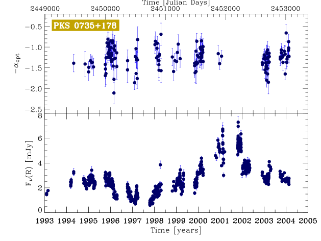
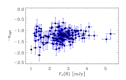
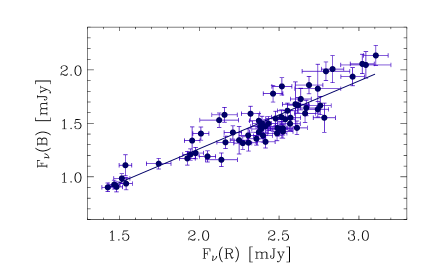
Figure 5: Upper panel: temporal behaviour of the optical spectral index $\alpha$ and the $R$-band flux in PKS 0735+178. This plot shows that the long–term variability is essentially achromatic, even if flares can imply spectral changes. Middle panel: dependence of the optical spectral index $\alpha$ on the flux intensity in the $R$-band. The scatter in the data can be explained as produced by statistical fluctuations due to instrumental and calculation errors, and by the intrinsic scatter of $\alpha$ during the more rapid and larger flares. A weak linear correlation is outlined. Lower panel: the scatter plot between the fluxes in $R$ and $B$ bands shows, as well, a linearly correlated emission (linear correlation coefficient $r_{B-R}=0.90\pm 0.18$ and slope $0.64\pm 0.04$).

7 Optical spectral indexes

The continuum spectral flux distribution of blazars in the optical range can be analyzed to distinguish properly all the emission components that, together with synchrotron radiation, contribute to the observed spectrum shape. Moreover optical flux variations in blazars are frequently associated by changes in the spectral shape. This can be revealed by analyzing the magnitude color indexes or the flux spectral indexes. In calculating the color indexes and the continuum spectral slopes, we selected the more accurate multi-band data (3 filter at least) about PKS 0735+178, obtained by a single telescope, and coupling frames with a maximum time lag of 20 minutes (in order to reduce possibly intrinsic/extrinsic, instrumental micro–variations). Since both the host galaxy of PKS 0735+178 and the feature possibly responsible for the intervening absorption at $z=0.424$ are rather faint (see sect. 2), it is reasonable to neglect the galaxy color interference and any thermal contribution in the observed continuum optical spectra. The observed magnitudes were transformed into flux densities, corrected by the Galactic absorption (derived by Schlegel, Finkbeiner, & Davis, 1998, see Tab. 2 lower panel) for the source (located at moderate Galactic latitude, b=18.07). The absorption is rather small (i.e. $B-I=0.8$ mag), accordingly the colour correction is little in comparison to the mean $B-I$ value of the source. Fluxes relative to zero-magnitude values are taken from the Johnson-Cousins system calibration presented in Bessell (1979, 1990) and Fiorucci & Munari (2003).

The optical spectral energy distribution (SED), can be expressed conveniently by a power law $\nu F_{\nu}\propto\nu^{-\alpha+1}$, ($\nu$ being the frequency of radiation and $\alpha$ the spectral index). In the optical regime the degree of correlation between $\alpha$ and the flux sheds light on the non-thermal emission processes (e.g. synchrotron and inverse-Compton processes), produced by a population of relativistic electrons in the jet. The degree of correlation between the spectral index $\alpha$ and the flux in various bands, through a least-square linear regression was checked, and values characterized by large errors and bad $\chi^{2}$ were rejected. We found that the spectral index $\alpha$ of PKS 0735+178 varies between $2.11\pm 0.26$ to $0.66\pm 0.20$, with an average value of $1.25\pm 0.15$ in the last ten years. These values for $\alpha$ are roughly in agreement with the values calculated previously in Fiorucci, Ciprini, & Tosti (2004) using only the Perugia Observatory data set.

In Fig.5 (upper panel) the temporal behaviour of $\alpha$ is represented in comparison with the flux light curve in the better-sampled $R$-band. The long–term variability seems essentially achromatic, and there is no obvious correlation between the light curve and the spectral index, whereas flares and short term variations can imply spectral changes. This is the same behaviour found in BL Lac (Villata et al., 2002, 2004) and in S5 0716+71 (Ghisellini et al., 1997; Raiteri et al., 2003). Unfortunately there is almost no spectral information during the 2001 outburst (lack of $B$ and $V$ data), to check a spectral flattening. The few data suggests a rather constant spectral index. In the same Fig.5 (middle panel) the scatter plot between $\alpha$ and the flux is reported. Data dispersion is evident, and can be explained as statistical fluctuations due to uncertainties and to scattering in $\alpha$ during the more rapid and larger flares. Such linear correlation seems weak and a general spectral flattening is not detected clearly. Uncorrelated random fluctuations in the emitted flux might introduce a statistical bias, due to the spectral index dependence by the flux (Massaro & Trevese, 1996), but values computed for the central frequency (close to the $R$-band, as plotted in Fig. 5), can be considered unbiased and representative of the brightness state. The spectral index $\alpha$ showed consistent variations even when the light curve has a rather small variations. On the contrary in the lower panel of Fig. 5 the scatter plot between the fluxes in the $R$ and $B$ bands shows a well correlated emission as expected (linear correlation coefficient $r_{B-R}=0.90\pm 0.18$ and slope $0.64\pm 0.04$), without a detectable curvature.

During well-defined and large flares at X-ray bands (especially observed in HBL), the X-ray spectral index versus the flux frequently displays a characteristic loop-like pattern (see, e.g. Georganopoulos & Marscher, 1998; Kataoka et al., 2000; Ravasio et al., 2004). That patterns outline a hysteresis cycle arising whenever the spectral slope is completely controlled by radiative cooling processes (see, e.g. Kirk, Rieger, & Mastichiadis, 1998; Böttcher & Chiang, 2002). In few sources this feature was found in the optical regime too (Fiorucci, Ciprini, & Tosti, 2004; Ciprini et al., 2004). Consequently we can claim that around and beyond the synchrotron peak frequency, the behaviour of the LBL sources during flares in the optical band, is scaled in frequency but possibly very similar to the behaviour of the HBL in X-rays bands.

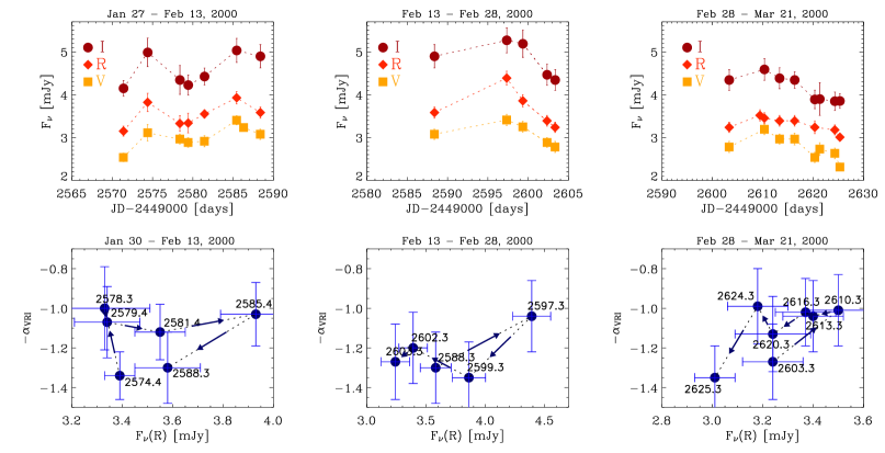
Figure 6: Evolution of the continuum optical spectrum of PKS 0735+178 (spectral index $\alpha$) as a function of the flux in $R$-band, during 3 contiguous periods of flickering variability with moderate flaring activity observed by the same telescope (Perugia Observatory, in period: January 29 - March 21, 2000). An approximative loop-like behaviour of $\alpha$ is hinted in the first (clockwise) and in the third (counterclockwise) patterns (see text for details).

In our 10-year light curve, PKS 0735+178 showed several moderate-amplitude outbursts, wider bump of longer duration, and a general flickering or shot-noise type of variability on mid-term scales. The evolution of $\alpha$ as a function of the flux is erratic and did not show evident hysteresis loops caused by non-thermal cooling. In Fig. 6 the evolution of $\alpha$ during 3 contiguous observing periods (from January 29, to March 21, 2000) is reported as example. A rough loop-like behaviour is hinted, meaning that radiative cooling can dominate the optical SED also during mild-flaring activity. Consequently variations at higher frequency band could lead those at the lower frequency bands during both the increasing and decreasing brightness phases, reflecting differences in electron cooling times.

The rather limited amplitude of the optical variability in the epochs of Fig. 6, the possible superimposition of different emission processes in the optical band, the under-sampling and the error propagation in the $\alpha$ calculation, can be the main reasons for the lack of well defined loops in such $\alpha$ vs flux diagrams. Our data are not sufficient to make a final judgement, and an improved multi-band monitoring and a better data sampling would probably clarify the existence of that patterns also during mild variability in this object.

8 Temporal variability analysis

Time series analysis (evolved from both signal-processing engineering and mathematical statistics) provides very useful methods to study blazar variability. These methods allows to explore and extract temporal signatures, structures and characteristic timescales (the powerful scales of variations), duty cycles (the fraction of time spent in an active state) and trends, to determine the dominant fluctuation modes and the power spectrum of the signal. Moreover time series analysis allows to detect and study auto/cross-correlations, time lags, transient events, periodicity and composite modulations, scaling and coherency, oscillations, beatings and instabilities, intermittence and drifts, dissipation, dumping, long-memory patterns and self-similarity, resonance and relaxation processes, random and deterministic features, linear and non-linear processes, stationary and non-stationary activity, as well as to perform filtering and forecast.

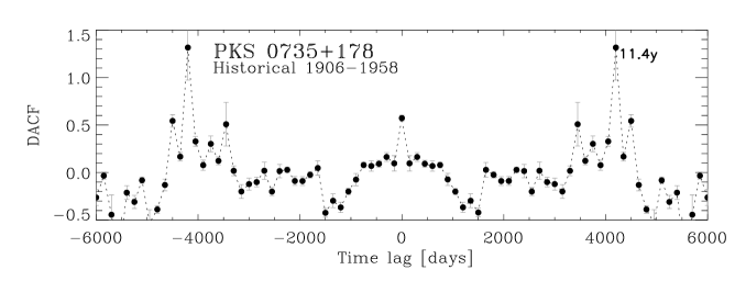
Figure 7: Discrete Autocorrelation Function (DACF; data bin: 7 days, DACF bin: 150 days) and Lomb-Scargle Periodogram (LSP; dashed line indicates the threshold of false alarm probability [FAP] fixed at 1%) of the pre-1970 light curve. A characteristic timescale around 11 years is hinted also by this poorly sampled portion of the historical light curve.

The analysis of the flux evolution over time in a blazar, joint with the multiwavelength and cross-correlation analysis, provides crucial information on the location, size, structure and dynamics of the emitting regions, and shed light on physical mechanisms of particle acceleration and radiation emission.

In this section a quantitative analysis of the optical variability observed in PKS 0735+178 is performed using 7 different methods in 13 different light curves. The aim of this work is to examine in detail the optical behaviour on long-term timescales (months/years) using the whole 1906-2004 historical light curve, the pre-1970 portion and the best sampled 1970-2004 part, and to explore mid-term scales (days/weeks in intervals $<200$ days) using our 10-year monitoring data set with improved sampling. Each seasonal light curve in the best sampled $R$-band is analyzed separately (a part of the first 2 pilot seasons, where we obtained only few observations). For the first time a rather comprehensive temporal analysis of the optical variability was performed over 3 decades in time in this peculiar blazar, investigating scales between about 2 and 30 years regarding the historical dataset, and between few days and about 100 days in the seasonal monitoring (the duration of season with data points spans between 144 and 203 days).

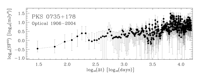
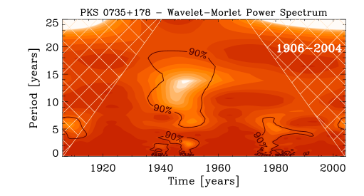
Figure 8: Panels from left to right and following below: the whole historical (1906–2004) flux light curve of PKS 0735+178 in $B$-band and plots from the related time-series analysis. First order Structure Function (SF; data bin: 7 day, SF bin: 60 days) in log-log representation, Discrete Auto Correlation Function (DACF; data bin: 7 day, DACF bin: 90 days), Lomb-Scargle Periodogram (LSP; dashed line is the 1% false alarm probability [FAP] threshold), “Clean” implementation of the Discrete Fourier Transform (CDFT), Phase Dispersion Minimization function (PDM), plane contour plot of the wavelet scalogram (i.e. the two-dimensional energy density function $\left|CWT(t,T)\right|^{2}$, CWT being the Continuous Wavelet Transform computed using a Morlet waveform, t and T the time and period scale respectively). In the last panel the periodogram of the synthetic light curve constructed upon the empty gaps using different window functions (GWFP; gap threshold 1 year). In the CWT scalogram the power spectral density is represented by filled-colour contour levels, while the thick black contours are the 90% confidence levels of true signal features against white/red noise background, and the cross-hatched regions represent the “cone of influence”, where edge effects become important. The descriptions of the plots above can be applied to the following Fig.9, Fig.10, Fig.11, and Fig.12. Issues and results from these diagrams are described in the text.

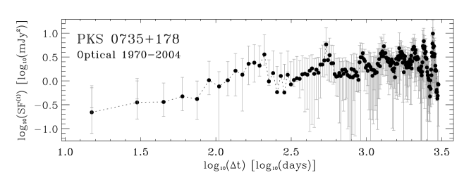
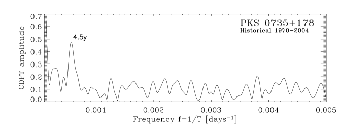
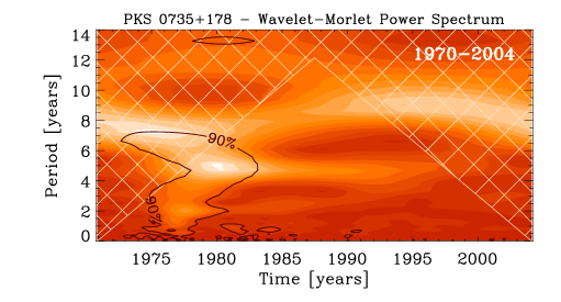
Figure 9: Panels from left to right and following below: the whole historical (1970–2004) flux light curve of PKS 0735+178 in $B$-band and plots from the related time-series analysis. SF (data bin: 1 day, SF bin: 15 days), DACF (data bin: 1 day, DACF bin: 60 days), LSP, CDFT, PDM, Morlet-CWT scalogram, and GWFP (gap threshold 0.3 years). Issues and results from these diagrams are described in the text.

The following methods, optimized or adapted for unevenly sampled timeseries, are applied: the first-order Structure Function (SF), the Discrete Auto Correlation Function (DACF), the Lomb-Scargle Periodogram (LSP), the Discrete Fourier Transform in the “Clean” implementation (CDFT), the Phase Dispersion Minimization (PDM), the scalogram of the Continuous Wavelet Transform (CWT) using different waveforms, and the periodogram of the synthetic light curve constructed on the empty gaps, using different window functions (Gaps Window Function Periodogram GWFP).

The SF is equivalent to the power spectral density function (PSD) of the signal calculated in the time domain instead of frequency space, which makes it less dependent on sampling problems, like windowing and alias (see, e.g. Rutman, 1978; Simonetti, Cordes, & Heeschen, 1985; Smith et al., 1993). The first order SF represents a measure of the mean squared of the flux differences $(F_{i}-F_{i+\Delta t})$ of $N$ pairs with the same time separation $\Delta t$:

$${\rm SF}^{(1)}(\Delta t)=\texttt{}\frac{1}{N}\sum_{i=1}^{N}\left(F_{i}-F_{i+\Delta t}\right)^{2}.$$ (1)

The general definition involves an ensemble average. Deep drops in the SF shape means a small variance and provides the signature of a possible characteristic time scales, but a wiggling pattern and fake breaks (that can indicate false time scales) are common when the sampling is not sufficient. Typically, the SF increases with $\Delta t$ in a log-log representation, showing an intermediate steep curve, whose slope $b$ is related to the power law index $a$ of the PSD by the relation $a=1+b$ (a typical PSD has indeed a power-law dependence $P(f)\propto 1/f^{a}$ on the signal frequency $f=1/t$). The maximum correlation timescale is reached when the SF is constant for longer lags (Hughes, Aller & Aller, 1992; Lainela & Valtaoja, 1993).

The DACF allows to study the level of auto-correlation in unevenly sampled data sets (see, e.g. Edelson & Krolik, 1988; Hufnagel & Bregman, 1992) without any interpolation or addition of artificial data points. The pairs $(F_{i},F_{j})$ of a discrete datasets are first combined in unbinned discrete correlations

$${\rm UDACF}_{ij}=\frac{(F_{i}-<F>)(F_{j}-<F>)}{\sigma_{F}\sigma_{F}},$$ (2)

where $<F>$ is the average values of the sample and $\sigma_{F}$, the standard deviation. Each of these correlations is associated with the pairwise lag $\Delta t_{ij}=t_{j}-t_{i}$ and every value represents information about real points. The DACF is obtained by binning the ${\rm UDACF}_{ij}$ for each time lag $\Delta t$, and averaging over the number $M$ of pairs whose time lag $\Delta t_{ij}$ is inside $\Delta t$, i.e.: ${\rm DACF}(\Delta t)=1/M\sum_{ij}{\rm UDACF}_{ij}$. The choice of the bin size is governed by a trade-off between the desired accuracy in the mean calculation and the desired resolution in the description of the correlation curve. A preliminary time binning of data usually leads to better results. The number of the real points per time bin can vary greatly in the DACF, but data bins with an equal population can be built together with Montecarlo estimations for peaks and uncertainties, as done in the Fisher $z$-transformed DACF method (ZDACF, Alexander, 1997).

The LSP is a technique analogous to the Fourier analysis for discrete unevenly sampled data trains, useful to detect the strength of harmonic components with a certain angular frequency $\omega=2\pi f$ (see, e.g. Lomb, 1976; Scargle, 1982; Horne & Baliunas, 1986; Papadakis & Lawrence, 1993).

In the CDFT method, first a “dirty” discrete Fourier transform (DFT) for unequally spaced data is calculated and then an interactive “cleaning” of the dirty DFT is performed (see, e.g. Högbom, 1974; Roberts, Lehar, & Dreher, 1987; Foster, 1995). The CDFT method is a complex and one-dimensional version of a deconvolution algorithm widely used in 2-dimensional image reconstruction. This technique provide a simple way to understand and remove false peak artifacts introduced by empty gaps. This method is effective especially in describing and recognizing multiperiodic signals. A standard (uncleaned) DFT method was implemented previously by Deeming (1975).

The PDM method (see, e.g. Lafler & Kinman, 1965; Jurkevich, 1971; Stellingwerf, 1978) try to minimize the variance of data at a constant phase with respect to the mean value of the light curve. If a trial period is close to a real period, the scattering of data against the derived mean in the light curve constructed on such phase (the light curve folded on such period) is small. The PDM method has no preference for a particular periodical shape, it incorporates all the data directly into the test statistic and it is well suited for small and randomly spaced samples. A value is statistically significant when the PDM drops towards zero.

The Wavelet method is used to transform a signal into another representation able to showing the information in a more useful shape (see, e.g. Daubechies, 1992; Foster, 1996; Percival & Walden, 2002). Wavelet transforms (WT) permits a local decomposition of the scaling behavior in time for each quantity (in contrast to the usual methods based on the Fourier analysis), allowing the signal features and the frequency of their “scales” to be determined simultaneously. Hence it is a useful tool especially to detect typical timescales and identify signals with exotic spectral features, transient information content and non-stationary properties. WT are defined following the Fourier theory, but wavelets can be formally described as localized, oscillatory functions whose properties are more attractive than sine and cosine functions.

WT is computed at different times in the signal, using mother wavelets (orthogonal base functions localized in both time and pulse spaces) of different frequency and convolved on each occasion. In this way the power spectrum (i.e. the modulus of the transform value) on a two dimensional location-frequency plane is obtained (the so called wavelet “scalogram”). A continuous WT of a one-dimensional (1D) time-series is computed as a complex array at different times, the real component being the amplitude and the imaginary component providing the phase. The square of the transformed modulus gives the wavelet power spectrum in function of both time and harmonic frequencies. In our analysis we chose the Morlet complex-valued waveform (see, e.g. Farge, 1992), composed of a plane wave modulated by a Gaussian envelope of unit width:

$$\psi_{0}(\tau)=\frac{1}{\sqrt[4]{\pi}}e^{i\omega_{0}\tau}e^{-\tau^{2}/2}$$ (3)

where $\tau$ is the non-dimensional time parameter and $\omega_{0}$ the non-dimensional frequency. Such continuous WT is convoluted on the discrete sequence of the time series $\{F_{i}\}$ with scaled and translated versions of $\psi_{0}(\tau)$. It is considerably faster to calculate such continuous WT in Fourier space: the convolution theorem allows to do all the N convolutions for a given scale simultaneously and efficiently in Fourier space N being the number of points in the time series) using a standard DFT (Kaiser, 1994; Percival & Walden, 2002).

The temporal analysis of the PKS 0735+178 optical dataset is performed using all the methods mentioned above separately on each light curve with results summarized in Table 3. In particular the diagrams from the time-series analysis of 5 light curves (the whole historical 1906-2004 and best sampled 1970-2004 $B$-band series, the seasonal IV, VII and X $R$-band light curves from our dataset) are reported in Fig. 8, Fig.9,Fig.10 Fig.11, and Fig.12. In the analysis of mid-term scales, the problem of spurious artifacts given by seasonal gaps with no data (solar conjunction with the source) was avoided studying each seasonal light curve separately. The GWFP of the best sampled 1970-2004 light curve (Fig.9 last panel, bottom, right) shows indeed only one powerful peak placed at exactly 1-year scale. This represents the periodical yearly recurrence of the seasonal gaps.

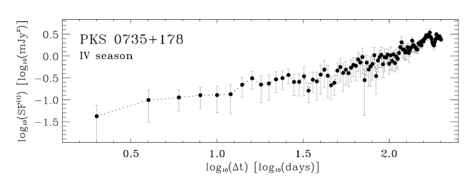
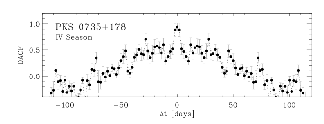
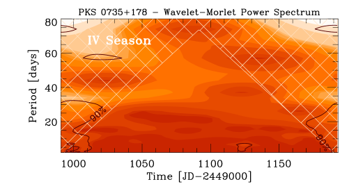
Figure 10: Panels from left to right and following below: the $R$-band light curve of PKS 0735+178 in the IV observing season (Sept. 1995, Apr. 1996) obtained by our monitoring programme, and related functions produced by the time-series analysis. SF (data bin: 1 day, SF bin: 2 days), DACF (data bin: 1 day, DACF bin: 2 days), LSP, CDFT, PDM, Morlet-CWT scalogram, and GWFP (gap threshold 5 days). Issues and results from these diagrams are described in the text. General results of the analysis of all the seasons from our dataset are summarized in Table3.

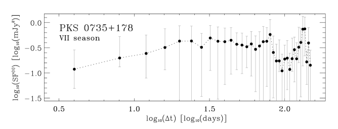
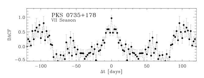
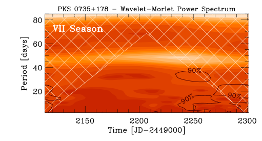
Figure 11: Panels from left to right and following below: the $R$-band light curve of PKS 0735+178 in the VII observing season (Oct. 1998, May 1999) obtained by our monitoring programme, and related functions produced by the time-series analysis. SF (data bin: 1 day, SF bin: 4 days), DACF (data bin: 1 day, DACF bin: 2 days), LSP, CDFT, PDM, Morlet-CWT scalogram, and GWFP (gap threshold 5 days). Issues and results from these diagrams are described in the text. General results of the analysis of all the seasons from our dataset are summarized in Table3.

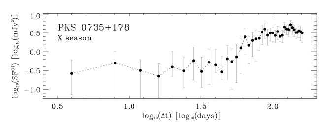
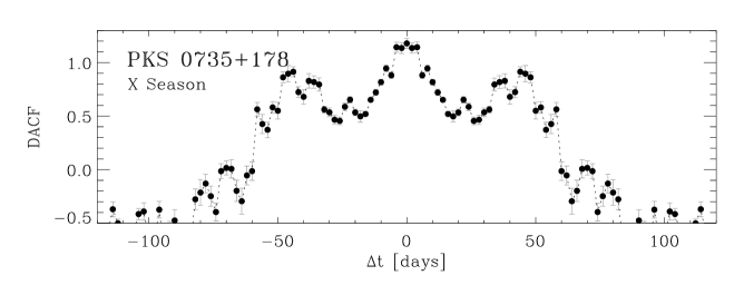
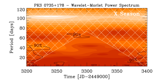
Figure 12: Panels from left to right and following below: the $R$-band light curve of PKS 0735+178 in the X observing season (Oct. 2001, May 2002) obtained by our monitoring programme, and related functions produced by the time-series analysis. SF (data bin: 1 day, SF bin: 4 days), DACF (data bin: 1 day, DACF bin: 2 days), LSP, CDFT, PDM, Morlet-CWT scalogram, and GWFP (gap threshold 5 days). Issues and results from these diagrams are described in the text. General results of the analysis of all the seasons from our dataset are summarized in Table3.

The whole 1906-2004 light curve (Fig. 8) is patently affected by substantial differences in data sampling, by void gaps, by a poor sampling earlier than 1970 and a long empty interval (1958-1970). Nevertheless several signal features and characteristic timescales are pointed out by the different techniques (using both binned and unbinned series): about 8.6y, 12-13y, 25y and 34y (see the summary reported in Table3). The 13.7y timescale (pointed out by nice features in the LSP and CWT functions) is the same value claimed as the major component of a multi-periodical trend by Qian & Tao (2004) and Fan et al. (1997), on the other hand the 8.6y timescale (suggested by the DACF and LSP) is probably to be ascribed mainly by the temporal behaviour after 1970 (Fig.9), and it is reported by Qian & Tao (2004) too. Longer duration scales (e.g. 34y) are difficult to be set out with confidence. Fake signal features, due to recurrences and temporal patterns given by the empty gaps, occurred at scales shorter than 8 years only (see the GWFP plot), therefore minor and fainter hallmarks in the SF, LSP, CWT corresponding to such shorter scales are neglected.

The best sampled portion of the historical light curve (1970–2004, Fig.9) spans 33 years and has a quite fair continuous, regular and long-term coverage: 867 nights with 1 datapoint at least, an average number of data points per night of 1.8, an average gaps among data of 7.8 days and a maximum gap of 1.6 years (Table3). The more relevant characteristic timescales suggested by the different temporal analysis methods are around 4.5y, 8.6y, and 12.5y (other few values such 3.5y, 7.4y, 11.8y years could be traced back to the previous mentioned, if we consider the finite-resolution accuracy of these methods). The 4.5, 8.6, 12.5 years scales might be considered multiples harmonic signatures of a fundamental (coherent, absolute, or transient periodical, or again with drifting duration) component of about 4 years (see also the spline visual envelope in Fig.13). A characteristic timescales of about 4.8 years was previously claimed also by Webb et al. (1988) and Smith et al. (1987), while the 8.6 years scale was recently suggested by Qian & Tao (2004). On the other hand no evidence for the periodical signature of 14.2 years previously claimed by Fan et al. (1997) are observed, but only weak hints for scales in the 11.6-13.5 years range are found out. The power spectral density in the $1/f^{a}$ regime, shows a slope index $a$ between 1.5 and 2 (i.e. next to a pure shot-noise behaviour). The GWFP show a very powerful fake signature at 1.0 years as expected, produced by the recurrent 1-year gap between subsequent observing seasons. This artifact due to sampling it is not completely neglected by the methods used (see e.g. the residual peaks around $\omega\sim 6$ i.e. $\sim 2\pi$ in the LSP plot), therefore it is very useful to develop and make use of the GWFP technique in conjunction with the other time series methods. No other (longer) fake features due to the irregular sampling are pointed out by the GWFP, therefore all the other characteristic timescales claimed in this light curve can be considered due to real variability. In the CWT scalogram a significant and localized pulse in power is visible (with a scale around 4.8 years and located in correspondence of the big 1977 outburst). Another localized bump gives a scale of about 7.4y. An elongated and lower intensity band in the CWT scalogram, corresponding to the last epochs (about 1994-2004) indicates again a coherent time scale between the values 8.2-8.9 years. Results are quite similar using different suitable CWT mother functions as the Mexican-hat and Paul waveforms in this light curve.

As example, in the time series analysis of the IV observing season of our $R$-band dataset (Sept. 1995, Apr. 1996, Fig.10) a main modulating trend quite monotonically decreasing is observed. This is stated for example by the shape of the SF in the logarithmic plot (second panel, top right of Fig.10) being quite linearly monotonic and without any turnover flattening (given by the reaching of a maximum correlation timescale). In this general trend 4 or 5 moderate and secondary oscillations can be visually identified (possibly related to the unique and weak signal of a characteristic timescale between 28-34 days, as hinted by the DACF, PDM, and CWT). Other characteristic scales are not displayed, and the artifact noise given by the irregular gaps, is important only at timescales below 13 days (see the GWFP last panel, bottom right). The power spectral density in the $1/f^{a}$ regime, shows a power index $a=1.97\pm 0.25$, i.e. a temporal variability mode like the shot noise (brown noise) signal.

In the $R$-band light curve during the VII observing season (Oct. 1998, May 1999, Fig. 11) a brightening stage (between about $JD=2451170$ and $JD=2451265$, i.e. 95 days long) looking as produced by two blended main flares of about 50 days duration, might be supposed by a visual inference. Such values (about 95 and 50 days) are pointed out indeed by the SF, DACF, LSP, PDM and CWT functions (Table3) as characteristic timescales (scales where is more power in the signal). The SF and PDM methods suggests also a possible timescale about 30 days. Fake features given by the irregular gaps are important only at timescales below 21 days (GWFP last panel, bottom right of Fig. 11). The power spectral density function shows a power index $a=1.64\pm 0.09$, i.e. a temporal fluctuation mode placed at halfway between the flickering and the shot noise behaviour.

The plots from the analysis of the X observing season data (Oct. 2001, May 2002, Fig.12) obtained by our monitoring programme, show an high state with two relevant flares, followed by a low and rather oscillating phase (after date $JD=2452273$). Unfortunately there was a long observing gap (about 25 days between $JD=2452218$ and $JD=2452243$) during the more active phase of this season, that is also the brightest optical state of the source recorded in our 1994-2004 database. Characteristic timescales of about 52-55 days are suggested by the LSP, CDFT, and PDM, while a 41 days scale is also found by the DACF and LSP (Table3). Fake features given by the irregular gaps are influential only at timescales below 18 days (GWFP last panel, bottom right, Fig.12). The power spectral density function shows a power index $a=1.46\pm 0.17$, i.e. again a temporal fluctuation mode placed at halfway between the flickering and the shot noise behaviour.

The summary of the temporal statistics and analysis results is showed in Table3. About statistics the following information is reported: the observing interval and its duration (98.1 years in total, and between 144 days and 203 days regarding our observing seasons); the number of the effective observing nights with one data point at least (867 data points in the 1970-2004 light curve, and between 20 and 62 in our dataset observing seasons); the average number of data points per observing night in the interval (spanning between 1 and 2.3, implying no data clustering); the average separation between 2 successive data points (3 days on average on all our 10 observing seasons); the maximum separation (maximum empty gap) between 2 successive data points (no more than 25 days in the worst sampled season). In time intervals where the SF slope can be recognized in the log-log representation, we calculated its power index $b$ trough a linear regression. About the time series analysis the following quantities are reported (when possible): characteristic timescales calculated by deep drops in the SF, the power law index $a=1+b$ of the PSD in the $1/f^{a}$ regime calculated by the SF, characteristic timescales inferred from the SF turnover to the plateau produced by times longer than the maximum correlation lag, timescales estimated from power peaks in the DACF/ZDACF, in the LSP and in the CDFT, timescales indicated by deep drops in the PDM and by peaks in CWT scalogram.

The criteria adopted in order to possibly avoid to quote fake features and artifacts due to the irregular sampling and gaps, or edge effects, in Table3 are the following: 1) only timescales shorter than 1/2 or 1/3 of the interval duration were considered; 2) only the more relevant signatures in each method are preliminary considered; 3) among these we discarded the features that are not indicated by more than one method on the same light curve portion, when the signature is not particularly strong; 4) if some timescales, among the remaining, is still matched by the synthetic GWFP, these are discarded too. Most of the applied methods take well into account the power of artifacts given by the irregular dataset and recurrences of gaps, as showed by Fig.8,9, 10,11, and 12 (see the comparison of the first 7 panels with the last GWFP panel). However residual spurious power can be still present in the functions (see e.g. the spurious peaks of the LSP around $\omega\sim 6$ i.e. $T=1$ year, in Fig.9 as mentioned).

On long timescales the main temporal components we found can be grouped in three main ranges of values: between 4.4 and 4.8 years, between 8.2 and 8.6 years and between 10.8 and 13.2 years (Fig.7,Fig.8, Fig.9 and Table3). These components could modulate the long term optical light curve of PKS 0735+178 with roughly cyclical oscillations. A characteristic timescale of about 4.8 years was previously claimed also by Webb et al. (1988) and Smith & Nair (1995) while a 8.6 years scale was recently suggested by Qian & Tao (2004). On the other hand we did not find any strong evidence of further and longer-duration ($>14$ years) timescales reported in literature (e.g. Fan et al., 1997; Qian & Tao, 2004, and Sect.2), but only weak hints of a 25 years and a 34 years signature.

Some parts of the light curve could contribute with different typical scales to the overall series, while data are treated in varying ways, with timescales suppressed or enhanced as the relative weight of different segments of the light curve changes. The variability scale of 8.2-8.6 years could be an important finding and a real signature of a dominant and possibly quasi-periodical component anyway, because it was found in both the whole 1906-2004 series and its best-sampled portion.

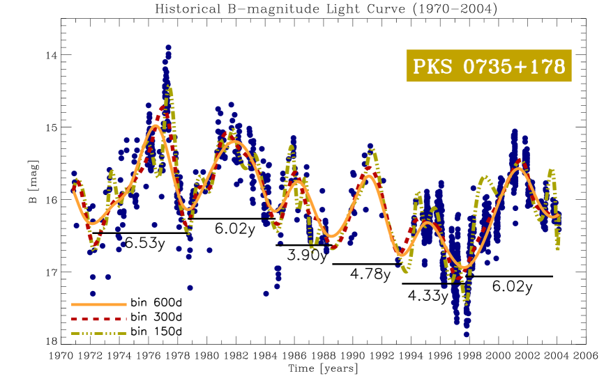
Figure 13: Cubic spline interpolations of the best sampled 1970-2004 historical light curve of PKS 0735+178. The continuous (orange) spline curve is obtained with a data binning of 600 days, while the other dotted/broken spline lines are obtained with binnings of 150 and 300 days. The interpolations show 6 main peaks already visible with the 600-days bin. With this binning and considering the separation between the troughs of the pseudo-sinusoidal curve, we have cycles of about 6.0-6.5 years and 3.9-4.8 years. This raw visual interpretation and spline envelope could be linked to one of the fundamental components (such as 4.4-4.8 years) found with the time series analysis (see Tab. 3). Hence both the hypotheses of a multi-component recurrent trend, or a pseudo-periodicity (with period drifts) and modulating this light curve can be plausible.

Moreover some uncertainty and statistical dispersion in the values found by different methods is expected, especially when the sampling is irregular, and here the dispersion range is small (0.4 years). In addition fast and/or isolated flares randomly occurred and uncorrelated to any general trend, can provide loud contributes to the power spectrum, disproving any periodicity hypothesis based on a long but under-sampled historical light curve. The better sampled portion of the PKS 0735+178 light curve did not disprove the characteristic timescale mentioned above, therefore it is reasonable to suppose a possible dominant period around 8.5 years. This hypotheses is open to future investigations based on prolonged monitoring observations. In this view the shorter 4.4-4.8 years scale found might be a submultiple of the previous component. Hence this would be the real period of the fundamental harmonics (pointed out only by the best sampled 1970-2004 portion because of the sufficient sampling to detect it). A support corroboration of this conjecture is also provided by the spline interpolation reported in Fig.13: 6 major maxima and cycles are outlined between 1970 and 2004, with a duration between 3.9-4.8 years and 6.0-6.5 years. This crude visual interpretation could be linked to the possible fundamental (and possible duration-drifting) modulating component of 4.5 years. Finally the group of longer-duration scales found in the broader range 10.8-13.2 years are detected in each piece of the historical light curve (see Tab. 3), but these values are probably too much scattered to mask a strict periodicity signature.

On intervals shorter than 200 days, monitored by our observations in 10 subsequent seasons (from the III starting in Oct.1994 to the XII ending in Feb.2004) and analyzed deeply with the methods mentioned above, there is no evidence for one single and pure periodical features, but there are signatures of several characteristic timescales of mid duration, commonly found in different observing seasons. These “recurrent” and “common” timescales are distributed in few groups of values: 18 days, 24-25 days, 27-28 days, between 40 and 42 days, between 50 and 56 days, 65-66 days, between 76 and 79 days, and 95-96 days. In particular the timescales of 27-28 days are found in 3 observing seasons (might be related to the synodical month interference), timescales between 50 and 56 days are observed in 6 seasonal light curves, and timescales between 76 and 79 days are detected in 4 seasons. About these timescales, several hypotheses can be proposed. 1) These temporal signatures could be the result of a rough multi-periodical behaviour given by the superimposition of few harmonic components (spanning from about 2 dozen of days to about 100 days). 2) They could be produced by pseudo-periodical cycles, with a drift of the period duration around a fundamental value of 27 days for example (50-56 and 76-79 days could be though as rough multiples in this case). 3) Such characteristic timescales could be produced by different periodical stages of transitory nature, with a sort of time-localized periodicity surviving only for limited epochs. 4) Again they could be the result of a variability mode endowed of few typical duty-cycles showing similar and recurrent peak shapes and durations, but occurring at random times. An improved and continuous monitoring, with an higher precision photometry and a better sampling, will provide more significant statistical results about the optical variability of PKS 0735+178 at these timescales.

9 Summary and conclusions

Blazars are one of the most exciting class of AGN, and the primary know extragalactic sources emitting high energy gamma-rays. Variability monitoring is an important effort in the study of blazars for several reasons (even if well sampled light curves are a very big challenge to be obtained at optical wavelengths normally).

Table 3: Summary of temporal statistics and characteristic timescales found in the optical light curves of PKS 0735+178 (when possible) using 7 different methods. Data sets investigated: 3 historical $B$-band flux light curves (the complete 1906-2004 curve, the best sampled 1970-2004 part, and the 1906-1958 portion), and 10 separated $R$-band flux light curves obtained in each observing season of our monitoring program (from the III season started in Oct.1994 to the XII season ended in Feb.2004). The following data are reported in the table columns (from left to right) for each light curve: (1) optical band and name of the light curve interval; (2) duration of the light curve; (3) number of the effective observing nights N_on with one data point at least; (4) average number of data points per observing night $<n>$; (5) average separation between two successive data points; (6) maximum separation (maximum empty gap) between two successive data points; (7) power-law index $a$ of the power spectral density ($PSD$) in the $1/f^{a}$ regime ($f=1/T$), calculated in the time-domain through the first order structure function $SF$; (8) characteristic timescales $T_{dr}$ calculated by deep drops in the $SF$; (9) characteristic timescales $T_{to}$ inferred from the $SF$ turnover to a long-lag plateau in the log-log representation; (10) timescales $T_{pe}$ estimated from peaks in the discrete auto-correlation function ($DACF$); (11) timescales $T_{pe}$ derived by peaks in the Lomb-Scargle periodogram $LSP$; (12) timescales $T_{pe}$ derived by peaks in the ‘clean” implementation of the discrete Fourier transform ($CDFT$); (13) timescales $T_{dr}$ estimated from deep drops in the phase dispersion minimization function $PDM$; (14) timescales pointed out by peaks in the 2-D contour plot of the wavelet scalogram (the two-dimensional energy density function provided by the continuous wavelet transform $CWT$ computed using a Morlet mother waveform). The errors in the timescales are difficult to be estimated in general, and the significance of a scale is high when it is relevant according to a method, and when several methods point out similar values. Columns from (2) to (5) show that the sampling is fairly regular without high data clustering. The criteria adopted in order to avoid possibly the quotation of fake features and artifacts due to the irregular sampling in this table, and results displayed here, are described in the text of the paper.

1) Short-term observations and multiwavelength (MW) snapshots obtained during broad but limited-duration campaigns cannot resolve all the puzzling questions about blazars, while long-term monitoring allows to investigate the behaviour and evolution of the emitted flux on different scales. 2) The knowledge about time variability is crucial like the spectral variability in constraint emission models, and the observed behaviour on long scales can be cross-correlated with the MW observations usually available on short timescales. 3) Radio-optical monitoring could be considered a farsighted effort too: it enable to construct long-term records of variability for several sources, useful for future researches. 4) Even if most of blazars seems to exhibit an irregular, uncorrelated and unpredictable temporal behaviour, their optical light curve shapes appear to be not trivial (sometimes signatures of long-term memory, temporal self similarity and intermittence are displayed), whereas in few known cases periodical/quasi-periodical components cannot be ruled out. 5) In addition, flare triggers and target of opportunity alerts for space observatories and large-size telescopes are usually based on a regular and constant monitoring. 6) Time series analysis of sparse data sets (like blazar light curves), is a challenging, interdisciplinary subject, being developed and applied on a wide variety of present-day research topics outside astrophysics. 7) Our fairly novel investigation and results on mid-term optical timescales (days, weeks), could be also compared to the analysis of blazar gamma-ray light curves that will be provided, at the same scales, by the forthcoming Gamma-ray Large Area Space Telescope (GLAST). In fact this high-energy space observatory will be a large field-of-view and all-sky monitor for flares and variability, allowing to record flux variations on over timescales $>1$ day on hundreds of $\gamma$-ray blazar-like sources. 8) Moreover worldwide international collaborations and the participation of amateur and schools/universities optical telescopes are now possible (thanks to the development of CCD photometry and automation technology) meaning a valuable link for education and public outreach.

With this in mind, during a long-term and painstaking optical monitoring programme, we have obtained, collected and analyzed the largest amount of optical data in 4 colors ever published on the prominent blazar PKS 0735+178, thanks to the collaboration of 3 professional observatories (Perugia, Torino and Tuorla) and 1 amateur facility (Sabadell). Furthermore a new $VRI$ photometric calibration of 7 comparison stars in the field of this blazar is presented (Tab. 1), joint with the reconstruction and analysis of the whole historical light curve (spanning now from 1906 to 2004). These optical data are rather unique with respect to continuity, sampling and duration for this source, and the associated data analysis enough comprehensive, despite of natural difficulties (weather/seeing conditions, seasonal gaps, technical problems or limited manpower). About 500 nights of observations, collected in more than 10 years (period 1993-2004), and providing 1332 new $BVRI$ final data points on PKS 0735+178 are reported and investigated, aiming to a quantitative statistical description of the data set, a characterization of the multi-band behaviour, and an investigation of variability over 3 decades in time, for the first time in this blazar.

During the last 10 years, PKS 0735+178 continued to show rapid and large–amplitude optical variations typical of blazars, even if the source remained in a rather low or intermediate brightness state (mag $R>14$), showing a mild flaring activity. However starting from the end of 1997 the source showed a clear increase of the average brightness until 2001, when an active phase occurred. In this decennium typical variations of about 2 mag in less than half-year are observed joint with a general wiggling pattern produced by a superimposition or succession of flares, and modulated by a slower (possibly achromatic and oscillating) long-term trend. The quiescent and mild-activity reported from 1994 to the second half of 2000 in the optical band, was also pointed out recently in radio bands, as a period of quiescent flux activity and highly twisted jet geometry (Agudo et al., 2006). In the whole $\sim$100-years history of PKS 0735+178 five brightest outbursts and active phases were observed: the last occurred in the period Feb.2001-Oct.2001, and the brightest outburst was observed in May 1977 (when the source reached its historical optical maximum $B\simeq 13.9$).

The analysis of the continuum optical spectrum of this blazar suggests, as expected, a correlation between the fluxes in $B$ and $R$ bands, while the long-term variability of the spectral index $\alpha$ appear to be essentially achromatic and independent by the wavelength (Fig. 5). High-amplitude and isolated flares can imply correlated spectral changes (usually a flattening, i.e. bluer when brighter), but our data showed usually a rather erratic evolution of $\alpha$ as a function of the flux, and few or weak hints of non-thermal signatures (see e.g. Fig. 6). At these mid-term timescales and without an increased sampling, it is reasonable to expect that the superimposition of pure synchrotron optical fluctuations and emission peaks cannot be easily disentangled from slower variability patterns produced by different mechanisms.

A summary of the quantitative temporal analysis performed in each single observing season of our $R$-band light curves is reported in Tab.3. Intervals $<200$ days are investigated discovering quite common characteristic scales of variability falling especially into value ranges of 27-28 days, 50-56 days and 76-79 days. These signatures are the stronger contribution to the power spectrum, possibly produced by correlated flares with typical duty cycles emitted by some charge/discharge-like mechanisms. On the contrary hand these typical timescales might represent the effects of single or few powerful random events that are completely uncorrelated and infrequent. On other words, even if a characteristic and intrinsic timescale is found, this does not mean necessarily a discovery of a dominant modulation or periodicity. In fact such evidence could well be produced by events of random or transitory nature, or be misrepresented by a combination of different underlying components affected by an insufficient observing sampling.

Moreover the shot–noise (Brownian/brown noise) behaviour, pointed-out by the values of the power-law index $a$ of the PSD (computed in each season and falling between 1.46 and 2.34, see Tab.3), reflects the nature of the variations and can be linked to the findings cited above. Red and brown noise are termed usually as $1/f^{a}$ (power-law decline) fluctuations, meaning that the occurrence of a specific variation is inversely proportional to its strength. Brownian variability can be produced by a sequence of random pulses endowed of long-term memory, where independent/discrete events and parallel relaxation processes (like shocks and knots, electron density fluctuations, magnetic field turbulence or plasma instabilities) might generate a succession of mild optical flares and oscillations with similar duty-cycles, on mid-term timescales. We remark that fluctuation in the statistical moments and parameters like the PSD and variance may be intrinsic in red/brown noise processes (see, e.g. Vio et al., 2005), even if our analysis is essentially phenomenological and model independent. In addition when we analyzed separately different segments of the light curve and applied methods like the wavelets, we took already into account non-stationarity problems.

About the historical behaviour of PKS 0735+178, we found 3 main characteristic timescales having an extension of about 4.5 years, about 8.5 years (possibly signatures of the same 4.5 years fundamental component) and between about 11 and 13 years (Table3). These scales could be the result of an oscillating and achromatic trend, modulating (with a pseudo-periodic or multi-component course) the long-term variability. Pseudo-periodicity can imply drifts in duration and modulation, while a multi-component trend has several different scales contributing in the composite modulation. In particular in the first hypothesis the majority of the the long-term characteristic timescales found might be multiple signatures of a base component slightly drifting and varying around the value of 4.5 years. The visual inference based for example on the light curves of Fig. 4 and Fig. 13, can supports this statistical finding. A rather “humped” or “multi-bumped” cyclical activity is evident, possibly meaning a bimodal course, defined by an alternation of active and quiescent stages. The limited temporal range of observations having a sufficient sampling (1970-2004) does not allow to understand if this pseudo-cyclical activity is a stable or transitory phenomena, and several hypotheses can explain the observed trend. A quasi/pseudo-periodical behaviour (with a fundamental component drifting/oscillating around a value of 4.5 years); a multi-component modulation (by possibly different correlated mechanisms); a mere random or transitory occurrence; a combination of the previous scenarios (for example a mixture of a multi-component trend with a quasi-periodical component). The achromatic behaviour reported in section 7, is in agreement with a dynamical model implying slower variations of the base level flux and long-term modulations, resulting for by variations in the beaming factor of the jet.

This kind of optical course could be better correlated to the radio flux behaviour and the twisted (maybe precessing) jet of PKS 0735+178 observed in details by some years. This peculiar blazar (both radio and X-ray selected, and also a gamma-ray EGRET source) shows quite slow variations in the radio bands and a complex morphology displaying several moving components. In previous literature the optical and radio history of PKS 0735+178 have already suggested a possible periodical activity. Periodicity in blazars has been debated for more than 40 years and several models were developed to explain this prospect (for example precessing or helical jets and supermassive binary black holes, see e.g. Lehto & Valtonen, 1996; Sillanpää et al., 1996; Villata et al., 1998; Rieger & Mannheim, 2000; Valtaoja et al., 2000; Ostorero, Villata, & Raiteri, 2004). However only in very few (and well publicized) cases there is still a sufficient evidence of cyclical outburst (like in OJ 287), and usually there is a general scepticism about widespread periodicity in quasars/blazars light curves till now. On the other hand the search for supermassive binary black holes in extragalactic sources, should become a major research topic in the next years.

As final consideration we point out that our 10-year observations probably mapped 2 distinct phases: a stage of low or intermediate optical luminosity (1994-2000) and a phase of mild flaring activity (2001). That dual and possibly cyclic scenario might well be confirmed by the behaviour of the radio flux and structure during the same years (Gabuzda et al., 1994; Gómez et al., 2001; Agudo et al., 2006). The optical flux is believed to be mainly originated in the very inner regions of the jet, even if the stronger variability could occur much farther from the central engine than previously expected (Marscher, 2005). Hence it is reasonable to conceive a correlation between the optical and radio flux on long-term scales, and during the most active events. An improved continuous and longer optical monitoring of PKS 0735+178, and the comparison of the optical flare events with the ejection and evolution of the superluminal radio knots based on long-term data records, will allow to shed light on the physics of the jet flow and flare mechanisms in this interesting object.