Properties of sunspots in cycle 23

Abstract

Aims. In this paper we investigate the dependence of umbral core brightness, as well as the mean umbral and penumbral brightness on the phase of the solar cycle and on the size of the sunspot.

Methods. Albregtsen & Maltby (1978) reported an increase in umbral core brightness from the early to the late phase of solar cycle from the analysis of 13 sunspots which cover solar cycles 20 and 21. Here we revisit this topic by analysing continuum images of more than 160 sunspots observed by the MDI instrument on board the SOHO spacecraft for the period between 1998 March to 2004 March, i.e. a sizable part of solar cycle 23. The advantage of this data set is its homogeneity, with no seeing fluctuations. A careful stray light correction, which is validated using the Mercury transit of 7th May, 2003, is carried out before the umbral and penumbral intensities are determined. The influence of the Zeeman splitting of the nearby Ni I spectral line on the measured “continuum” intensity is also taken into account.

Results. We did not observe any significant variation in umbral core, mean umbral and mean penumbral intensities with solar cycle, which is in contrast to earlier findings for the umbral core intensity. We do find a strong and clear dependence of the umbral brightness on sunspot size, however. The penumbral brightness also displays a weak dependence. The brightness-radius relationship has numerous implications, some of which, such as those for the energy transport in umbrae, are pointed out.

1 Introduction

Albregtsen & Maltby (albregtsen1 (1978), cf. Albregtsen & Maltby albregtsen2 (1981), Albregtsen et al. albregtsen (1984)) reported a dependence of umbral core brightness on the phase of the solar cycle based on 13 sunspots observed at Oslo Solar Observatory. The umbral core is defined as the darkest part of the umbra. According to their findings, sunspots present in the early solar cycle are the darkest, while as the cycle progresses spots have increasingly brighter umbrae. Also, the authors did not find any dependence of this relation on the size or the type of the sunspot. Following this discovery Maltby et al. (maltby (1986)) proposed three different semi-empirical model atmospheres for the umbral core, corresponding to early, middle and late phases of the solar cycle.

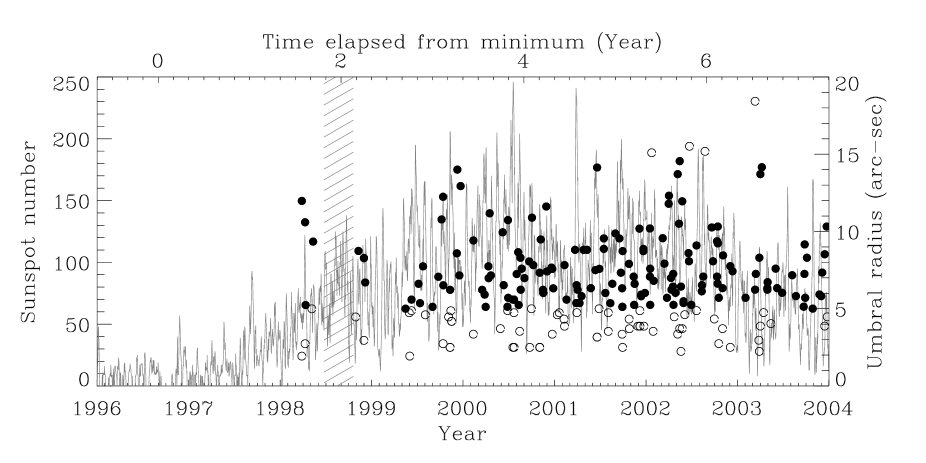
Figure 1: Distribution of analysed sunspots over the ongoing solar cycle 23. The grey solid line shows the International Sunspot Number (left scale). The solid circles show the dates of observation and umbral radii of the analysed sunspots with umbral radii between 5 and 15 arc-sec, and the open circles show the sunspots with umbral radii less than 5 arc-sec or greater than 15 arc-sec (right-hand scale). No sunspot in 1996 & 1997 fulfilled the selection criteria of $\mu>0.94$. The hatched area marks the period when contact with SOHO was lost.

In order to explain the umbral brightness variation with solar cycle two hypotheses have been put forward. Sch$\mathrm{\ddot{u}}$ssler (schussler (1980)) proposed that umbral brightness may be influenced by the age of the sub-photospheric flux tubes, whereas Yoshimura (yoshimura (1983)) suggested that the brightness of the umbra depends on the depth in the convection zone at which the flux tube is formed. Confirmation of these results appears important for two reasons. Firstly, this is the only strong evidence for a dependence of local properties of the magnetic features on the global cycle. E. g., the facular contrast does not depend on solar cycle phase (Ortiz et al. ortiz (2006)). Secondly, such a confirmation appears timely in the light of the recent paper by Norton & Gilman (norton (2004)), who reported a smooth decrease in umbral brightness from early to mid phase in solar cycle 23, reaching a minimum intensity around solar maximum, after which the umbral brightness increased again, based on the analysis of more than 650 sunspots observed with the MDI instrument. This decrease in brightness contradicts the results of Maltby et al. (maltby (1986)). Also, the data used by Norton & Gilman (norton (2004)) were not corrected for stray light and no sunspot size dependence of the brightness was discussed.

In this paper we investigate the dependence of umbral core brightness, as well as the mean umbral and penumbral brightness on the solar cycle and on the size of the sunspot. In the following section we describe the data selection. In the third section we deal with the data correction for stray light and for the influence of Zeeman splitting of the nearby Ni I absorption line on continuum measurements. In sections 4 and 5 we present our results. We discuss our results and compare them with earlier findings in section 6.

2 Data selection

Continuum full disk images recorded by the Michelson Doppler Imager (MDI; Scherrer et al. scherrer (1995)) on board the SOHO spacecraft are used in this analysis. The continuum images are obtained from five filtergrams observed around the Ni I 6768 Å mid-photospheric absorption line with a spectral pass band of 94 mÅ each. The filtergrams are summed in such a way as to obtain the continuum intensity is free of Doppler cross talk at the 0.2% level. The advantage of this data set is its homogeneity with no seeing fluctuations.

We selected 234 sunspots observed between March, 1998 and March, 2004. The selected sunspots were located close to the disk centre, i.e. for $\mu>0.94$, where $\mu=\cos\theta$ and $\theta$ is the angle between the line-of-sight and the surface normal. Also, our analysis was mostly restricted to regular sunspots, this excluded complex sunspots having very irregular shape and multiple umbrae. By looking through the daily images and selecting the sunspot when it was very close to the central meridian, we make sure that a particular sunspot is included only once in our analysis during one solar rotation. Out of the selected sunspots, 164 sunspots have an umbral radius between 5″ and 15″. Even though all the 234 sunspots were used for the study of radius-brightness dependence, only the sunspots with umbral radius between 5″ to 15″ were used for the study of brightness dependence on solar cycle. This is done in order to facilitate a direct comparison of our results with those of Maltby et al. (maltby (1986)). The data set covers most of solar cycle 23, although it does miss a few sunspots in the beginning of the cycle due to our selection criteria and the end of the cycle.

Figure 1 shows the distribution of sunspots over cycle 23, used for the study of the solar cycle dependence of brightness (filled circles) and those used only to determine the dependence on size (open circles). By restricting the analysis to sunspots near the disk centre, we avoid the suspected effect of centre-to-limb variation on the umbral brightness (Albregtsen et al. albregtsen (1984)). This is shown in Sect. 5.

The determination of umbral-penumbral and penumbral-quiet sun boundaries was carried out using the cumulative histogram (Pettauer & Brandt pettauer (1997)) of the intensity of the sunspot brightness and of the immediately surrounding quiet Sun (whose average is set to unity). This histogram was computed for 88 symmetric sunspots scattered across the observational period and then averaged. This averaged cumulative histogram is shown in Fig. 2. Note that the histogram is computed after stray light correction (see Sect. 3). The quiet Sun corresponds to the steep rise around normalised intensity unity. The rise at around 0.6 corresponds to the penumbra, below that is the umbra. In order to determine the intensity threshold corresponding to the penumbra-photosphere and umbra-penumbra boundaries linear fits to the flattest parts of the averaged histogram were computed. The boundaries were chosen at the highest intensity at which the linear fit ceases to be a tangent to the histogram. The reason why the penumbra is visible as a reasonably sharp drop, while the umbra is not, is only partly due to the larger range of intensity found in the umbra. It is mainly due to the large difference in umbral brightness from spot to spot (see Sect. 4). From the average cumulative histogram it was found that values of 0.655 and 0.945 in normalised intensity correspond to umbral-penumbral, and penumbral-quiet sun boundaries, respectively. These values were later used to determine the umbral and spot radius. All intensities are normalised to quiet Sun values at roughly the same $\mu$ value as the sunspot.

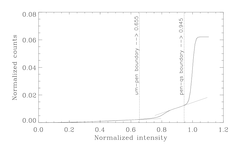
Figure 2: Average cumulative intensity histogram used for obtaining the umbral-penumbral and penumbral-quiet Sun sunspot boundaries. Dotted lines are linear fits to the flattest parts of the histogram. Vertical dotted lines mark the values selected for umbral-penumbral and penumbral-quiet Sun boundaries.

Figure 3: Off-limb stray light profiles of SoHO/MDI continuum images for 8 different years.

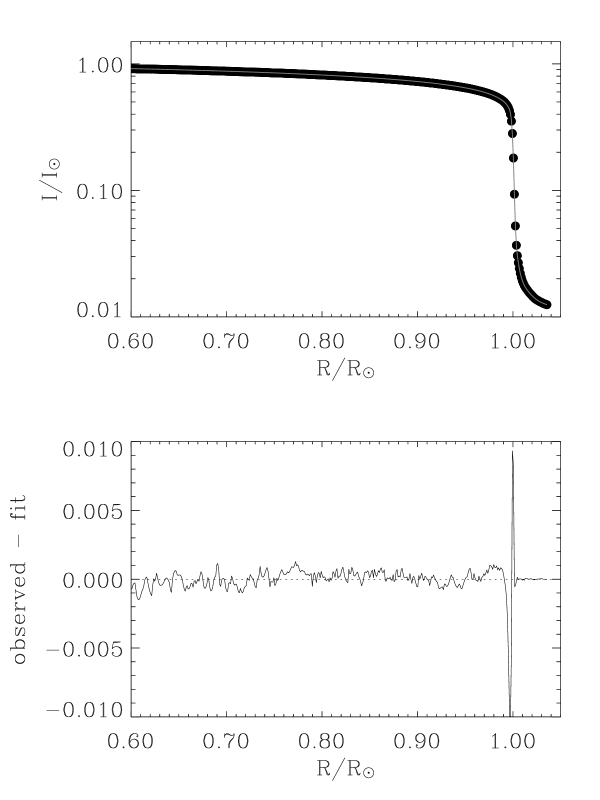
Figure 4: A typical stray-light fit to the observed limb profile. Top: the filled circles show the observed average limb profile and the solid line shows the fit to the observed profile. Bottom: the residual after the fit.

3 Data correction

Before retrieving the brightness, we made a few corrections to the observed data. Even though the atmospheric seeing related blurring and distortions are absent, MDI continuum images are found to be contaminated by instrumental scattered light. By checking the falloff of intensity just outside the solar limb, it was noticed that the instrumental scattered light increased with the aging of the instrument, which we carefully correct for.

Also, continuum measurements in MDI are not carried out in a pure continuum spectral band. As described in the previous section, five filtergrams obtained around a Ni I absorption line are used to compute the continuum intensities. We investigate the effect of this absorption line in the vicinity of a filter pass-band on observed continuum intensities. This is especially important in sunspots where the line profile changes due to the presence of a magnetic field. In the following subsections we elaborate on these corrections.

3.1 Stray light correction

In order to remove the stray light, average radial profiles were obtained from the observed full-disk MDI continuum images. Figure 3 shows such intensity profiles obtained from an MDI continuum image, averaged over the whole limb, each year just outside the solar disk. The gradual increase in scattered light with time is clearly evident in the plot. These profiles were fitted to retrieve the PSF (point-spread function) of the instrument (Martínez Pillet valentin (1992), Walton & Preminger walton (1999)). The radial profiles were generated using the spread function along with the centre-to-limb variation (CLV). A fifth order polynomial is used to describe the CLV. The initial values of the CLV coefficients were taken from Pierce & Slaughter (pierce (1977)). The computed profiles were iteratively fitted to the observations by adjusting the coefficients of the PSF and CLV. A deconvolution of the observed image with the model PSF (generated from the fitted coefficients) is carried out to retrieve the original intensity.

Figure 4 shows a typical fit to the observed radial profile and the difference between observed and fitted profiles. The spikes in the residual are due to the sharp change in intensity at the solar limb and are restricted to the points just outside and inside the Sun. Excluding these points, the residuals always lie between $\pm 0.002$.

We tested our fitting procedure for the stray light correction using MDI continuum images of the Mercury transit on 7th May, 2003. Figure 5 shows the observed and restored intensity for a cut across the solar disk through the Mercury image (at $\mu=0.65$) whose expected full width at half maximum is 12″, i.e. typical of the diameter of a sunspot umbra. It is evident from the figure that while the intensity in the original cut through the Mercury image never drops below 16%, after the stray light removal the intensity drops to very close to zero. More details of the stray light correction are given in Appendix A.

Figure 5: Observed and restored intensity for a cut across the solar disk through the Mercury image. Filled circles show the observed intensity profile through the centre of the mercury image. The solid line shows the profile after the stray light removal.

3.2 Correction for the Zeeman splitting of the Ni I line

In MDI, the continuum is computed by measuring intensities at five filter positions (designated as F₀ through F₄, cf. Scherrer et al. scherrer (1995)) on a spectral band which includes the Ni I absorption line. The filter F₀ (whose profile is shown in Fig. 6) gives the main contribution to the measured continuum, while the intensities recorded through the other filters are used to correct for intrusions of the Ni I line into the continuum filter, mainly introduced by Doppler shifts. The claimed accuracy for such corrections is 0.2% of the continuum intensity (Scherrer et al. scherrer (1995)), which is perfectly adequate for our analysis.

Figure 6: Synthesised Ni I line profiles (solid lines). Filled circles represent the FTS quiet Sun (QS) spectrum for the same line. The dashed curve shows the position of the MDI-F₀ filter transmission profile.

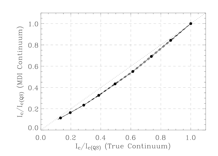
Figure 7: Brightness correction for the contribution of the Ni I line to the MDI-continuum measurements. The solid line shows the normalised continuum intensity computed including the influence of the spectral line plotted versus the computed true continuum for the same set of model atmospheres. Dashed lines are for magnetic field strengths around 10% below or above the values listed in Table 1, for a given value of temperature.

It is, however, not clear to what extent the Zeeman splitting of the line, as known to be present in sunspots, affects the continuum intensity measurement. In order to quantify this effect in sunspots, we carried out a series of calculations taking various values for magnetic field strength and temperature, which approximately simulate the relationship between the magnetic field and corresponding temperatures found in sunspots following Kopp & Rabin (kopp (1992)), Solanki et al. (sol1993 (1993)), and Mathew et al. (mathew (2002)). The exact choice of the field strength-temperature relation is not very critical, as we have found by considering also other combinations (e.g. with lower or with higher field strength for a given temperature). The magnetic field strength and the corresponding temperature along with other parameters used in the synthesis of Ni I line profiles are given in Table 1. The abundance is given on a logarithmic scale on which the hydrogen abundance is 12 and the oscillator strength implies the $\log(gf)$ value.

Table 1: Parameters used for producing Ni I line profiles

Centre wavelength	6767.768 Å
Abundance (Ni)	6.25
Oscillator strength	$-$1.84
Macro turbulence	1.04 km s-1
Micro turbulence	0.13 km s-1
Temperature (K)	Field strength (G)
5750	0
5500	1100
5250	1700
5000	2250
4750	2250
4500	2500
4250	3000
4000	3500
3750	4000

Figure 8: The change in full width (solid line; left scale), equivalent width (dotted line; left scale) and line depth (dashed line; right scale) with effective temperature.

Figure 6 shows the computed Ni I line profiles along with the position of the MDI-F₀ filter transmission profile. The solid circles are the quiet Sun FTS (Fourier Transform Spectrometer) spectrum for the same line (Kurucz et al. kurucz_at (1984)). Each plotted line profile was computed using a model atmosphere from Kurucz (kurucz (1991)) with effective temperature and height independent vertical magnetic field of the strength listed in Table 1. The Ni abundance is taken from Grevesse & Sauval (grevesse (1998)) and the atomic parameters are obtained from the Kurucz/NIST/VALD atomic data bases. As a first step, the Ni I line profile taken from the quiet Sun FTS spectrum is fitted using the Kurucz quiet Sun model atmosphere (T${}_{\rm eff}=$ 5750 K) keeping the micro- and macro-turbulence and oscillator strength as free parameters. The values obtained for the oscillator strength and micro- and macro-turbulence from the fit are maintained when computing all the remaining line profiles with various magnetic field strengths. MDI theoretical filter transmission profiles are created for the five filter positions across the spectral line. The transmitted intensity through each filter is computed and combined following Scherrer et al. (scherrer (1995)) to derive the continuum intensities. In Fig. 7 we plot the ‘true continuum’ intensities (i.e., the intensity which would have been measured through the filter if the line were not present in the vicinity of the MDI filter) versus the intensities resulting from the MDI continuum measurements for different effective temperatures. Clearly, the MDI continuum measurements in the presence of the Ni I absorption line provide a lower intensity than the real continuum in the sunspots, and the difference varies with the changing field strength and temperature. Naively one would expect this difference to increase for increasing magnetic field strengths, whereas the actually found behaviour is more complex. An explanation for this is given in Fig. 8. The decreasing temperature reduces the line depth (which is given in units relative to the continuum intensity for the relevant line profile), while the equivalent width initially increases before decreasing again with decreasing temperature if the field is left unchanged. Increasing field strength leads to enhanced line broadening and a slight increase in equivalent width. The combined influence of both effects is plotted in Fig. 8. Note that the width is measured as the wavelength difference between the two outer parts of the line profile at which it drops to $1-d/2$, where $d$ is the line depth in units of the continuum intensity. The behaviour seen in Fig. 7 therefore partly reflects the dependence of the equivalent width on temperature, but quite significantly also the fact that the total intensity absorbed by the line in terms of the continuum intensity of the quiet Sun decreases rapidly with decreasing temperature. This is the quality more relevant for our needs, rather than total absorbed intensity relative to sunspot continuum intensity, which corresponds to the equivalent width.

Figure 9: Cut through two simple sunspots with different effective umbral radii of around (a) 15 arc-sec and (b) 6 arc-sec.

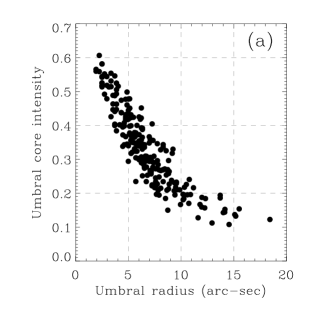
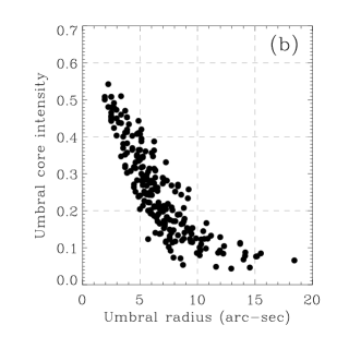
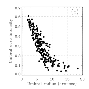
Figure 10: Umbral core intensity versus umbral radius, (a) observed, (b) corrected for stray light, and (c) corrected for stray light and the influence of the Ni I line. Here sunspots with umbral radius less than 5 arc-sec and greater than 15 arc-sec are also included.

The two dashed lines in Fig. 7, which are hardly distinguishable from the solid line correspond to using different field strength-temperature relations. The upper one is found if we decrease the field strength by around 10% (i.e. the correction is minutely smaller), the lower one for around 10% higher field. We use the solid line in Fig. 7 to correct the observed continuum intensities in sunspots. During the data reduction process all the resulting intensities after the stray light removal are replaced by reading out the corresponding value from the computed true continuum.

4 Brightness-radius relationships

Before discussing the brightness-radius relationship,in Fig. 9 we show cuts through two different sunspots. Those allow us to point out various intensity values used in our study. The big sunspot (Fig. 9(a)) has an effective umbral radius of around 15″. The horizontal dashed lines indicate the umbral and penumbral boundaries, whereas the dotted lines represent mean and minimum umbral intensities as well as mean penumbral intensity in this particular sunspot. Similarly, Fig. 9(b) shows a cut through a small sunspot (umbral radius $\approx 6$″).

4.1 Umbral core and mean intensity versus umbral radius

Figure 10 shows the relation between umbral core intensity and umbral radius. The umbral radius is computed as the radius of a circle with the same area as the (irregularly shaped) umbra under study. The umbral core intensity is the lowest intensity value found in the particular umbra (see Fig. 9).

All intensities are normalised to the average local quiet Sun intensity. Figure 10(a) shows this relation for the observed intensity and (b) for the stray light corrected intensities. The influence of the Ni I line on the continuum measurement is still present in this panel. Figure 10(c) is corrected for both the stray light and the effect of the Ni I line on the continuum measurement. In all the figures the trend remains the same. It is clear from the figure that the core intensity decreases very strongly with increasing umbral radius.

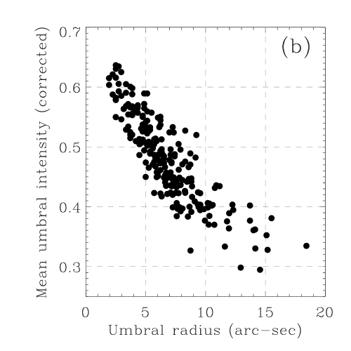
Figure 11: Mean umbral intensity versus umbral radius, (a) observed and, (b) corrected for stray light and the influence of the Ni I line. Here sunspots with umbral radius less than 5 arc-sec and greater than 15 arc-sec are also included.

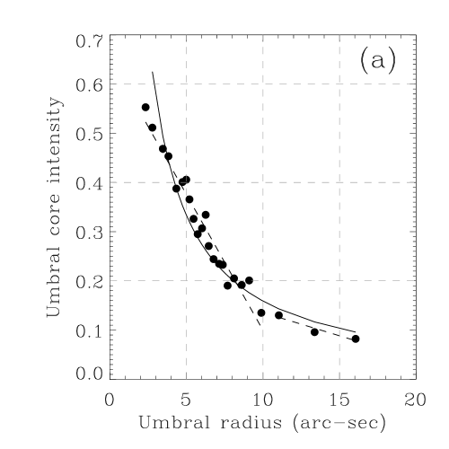
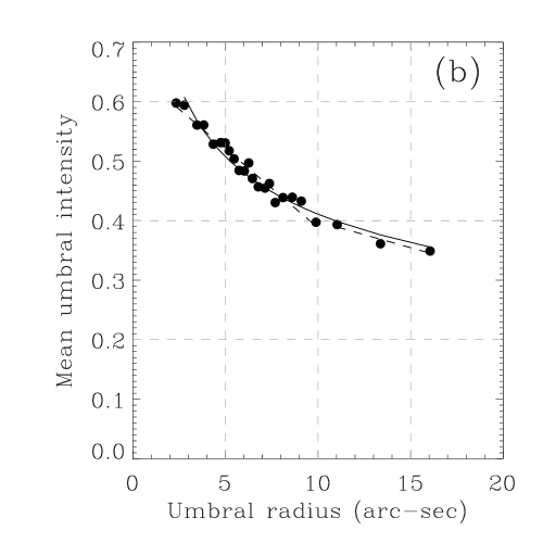
Figure 12: Power law fit (solid line) and double linear fit (dash lines) to the (a) umbral core intensity and, (b) mean umbral intensity. Here the filled circles represent bins of 10 spots each.

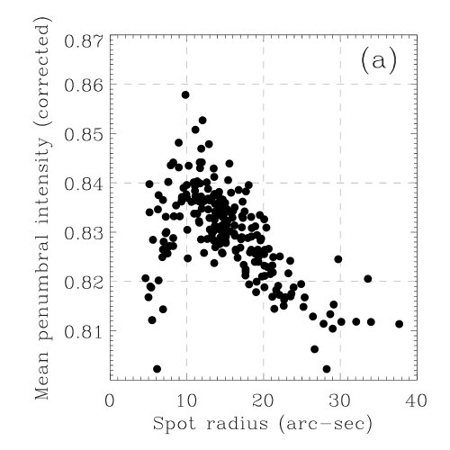
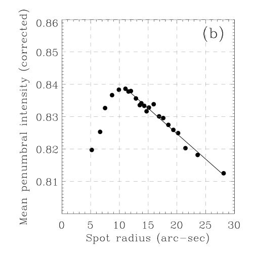
Figure 13: (a) Mean penumbral intensity versus spot radius, corrected for stray light. (b) Linear fit to the binned mean penumbral intensity.

Table 2: Fit parameters for radius-brightness relation

Dependence on umbral radius of,	Umbral radius	Constant	Exponent	Gradient	$\sigma$	$\chi^{2}$
Power law fit
umbral core intensity	(all)	1.8598	$-1.0679$		0.063	$3.5\times 10^{-3}$
umbral mean intensity	(all)	0.8297	$-0.3052$		0.013	$1.5\times 10^{-4}$
Double linear fit
umbral core intensity	$<$10′′	0.6515		$-0.0552$	0.0029	$6.7\times 10^{-4}$
	$>$10′′	0.2299		$-0.0094$	0.0027	$4.7\times 10^{-5}$
umbral mean intensity	$<$10′′	0.6536		$-0.0266$	0.0013	$1.2\times 10^{-4}$
	$>$10′′	0.4858		$-0.0087$	0.0026	$4.3\times 10^{-5}$
Dependence on spot radius of,
Linear fit
penumbral mean intensity	$>$10′′	0.8561		$-0.0016$	0.0001	$1.1\times 10^{-6}$

A steeper decrease is found for spots with smaller umbral radius, while for the bigger spots a more gentle decrease in umbral core intensity with radius is observed (dictated by the fact that umbral intensity has to be positive). This plot emphasises the need to take into account the dependence of the umbral brightness on the size of the spot when looking for solar cycle variations.

The mean umbral intensity, plotted in Fig. 11, also shows a similar decrease with increase in umbral radius. The difference between the umbral core and mean intensities is smallest for the smallest umbrae and increases with umbral size.

In order to obtain a relation between the umbral core and mean intensities with umbral radius, we carried out two different fits to the respective corrected umbral intensities after binning together points with similar sunspot radius, such that each bin contains 10 samples. The dashed lines in Figs. 12(a) and (b) show the double linear fits to the umbral core and mean intensities, respectively. The individual linear fits are made to spots with umbral radii less than 10″ and to those with radii above this limit, respectively. The fit parameters along with errors and normalised $\chi^{2}$ values are included in Table 2. The solid lines in these figures show the power law fit. The power law fit to the umbral core intensity seems to be a comparatively poor approximation, while the mean umbral brightness seems to obey the power law (i.e. it gives a very low $\chi^{2}$ for half the number of free parameters as the double linear fit). The parameters for the power law fit are also included in Table 2. Figure 12 again demonstrates that the difference between the core and mean intensity increases rapidly with umbral radius. It is equally clear that since the umbral core intensity varies by a factor of nearly 6, the mean umbral intensity by a factor of nearly 2 between the smallest and the largest umbrae, employing a single value for umbral brightness of all spots is a very poor approximation. Such an approximation is often made e.g. for the reconstruction of solar irradiance (cf. Unruh et al. unruh (1999), Krivova et al. krivova (2003)).

4.2 Penumbral mean intensity and spot radius

Figure 13(a) shows the relation between mean penumbral intensity and spot radius. An approximate linear relationship is evident for the spots with outer penumbral radius between 10″ and 30″. The outer penumbral radius is the equivalent radius of the whole sunspot (including the umbra). The large scatter in mean penumbral intensities for spot sizes below 10″ might result from the insufficient resolution of the full disk images or may be due to the fact that the parameters for distinguishing between umbra and penumbra are possibly not appropriate for small spots. Note the order of magnitude smaller range of variation of penumbral contrast than of umbral contrast. Figure 13(b) shows the linear fit to the mean penumbral brightness, after binning 10 adjacent spots (taking only spots with radius greater than 10^′′). The fit parameters are listed in Table 2.

Figure 14: Umbral core intensity versus solar cycle, (a) observed, (b) corrected for stray light, and (c) corrected for stray light and the influence of Ni I line. The intensities are plotted for all spots with umbral radii between 5 arc-sec and 15 arc-sec. The solid line shows the linear regression and the dashed lines represent the $\pm 1\sigma$ deviation, due to the uncertainty in the regression gradient. The best linear fit is given in the upper left corner.

5 Solar cycle dependence of the brightness

In Fig. 14 we plot the sunspot umbral core intensity versus time elapsed since the solar cycle minimum. September 1996 is taken as the minimum month, the upper axis shows the corresponding year. This plot includes spots with umbral radius between 5″ and 15″ only, in order to be consistent with the work of Albregtsen & Maltby (albregtsen1 (1978)). Figure 14(a) shows the observed intensity, (b) the stray light corrected intensity, while Fig. 14(c) shows the intensity corrected for both stray light and the influence of the Ni I line on the continuum measurements. In all the figures the trend remains the same. As the umbral radius and core brightness are related, the scatter in one quantity also reflects the scatter in the other.

The solid line shows the linear regression to the brightness, whereas the dotted lines indicate the 1$\sigma$ error in the gradient. A feeble trend of increasing umbral brightness towards the later phase of the solar cycle is observed. This increase is well within the 1$\sigma$ error bars and statistically insignificant. Table 3 lists the fit parameters, including the errors and normalised $\chi^{2}$ values. All the fit parameters are listed for the corrected intensity values. Also, in all the remaining figures we plot the corrected intensities alone.

Figure 15: Umbral core intensity versus solar cycle plotted for (a) umbral radii ranging from 5 to 10 arc-sec and, (b) from 10 to 15 arc-sec. The solid lines show the regression fits and the dashed lines the $\pm 1\sigma$ deviations due to the uncertainty in the regression gradient.

Table 3: Fit parameters for solar cycle dependence

Solar cycle dependence of,	Umbral radius	Constant	Gradient	$\sigma$	Gradient$/\sigma$	$\chi^{2}$
umbral core intensity	(all)	0.33605	$-0.00785$	0.00649	$-1.2095$	0.01901
	5′′ - 15′′	0.22188	$+0.00358$	0.00577	$+0.6205$	0.01015
	5′′ - 10′′	0.25001	$+0.00227$	0.00582	$+0.3900$	0.00841
	10′′ - 15′′	0.12560	$-0.00269$	0.00547	$-0.4918$	0.00158
	(all, northern hemisphere)	0.33957	$-0.01071$	0.00622	$-1.7218$	0.00085
	(all, southern hemisphere)	0.33062	$-0.00310$	0.00874	$-0.3547$	0.00164
umbral mean intensity	5′′ - 15′′	0.44346	$+0.00206$	0.00312	$+0.6603$	0.00296
	5′′ - 10′′	0.45782	$+0.00168$	0.00294	$+0.5714$	0.00215
	10′′ - 15′′	0.39609	$-0.00333$	0.00513	$-0.6491$	0.00139
penumbral mean intensity	5′′ - 15′′	0.82974	$-0.00009$	0.00049	$-0.1837$	0.00007
	5′′ - 10′′	0.83324	$-0.00034$	0.00042	$-0.8095$	0.00004
	10′′ - 15′′	0.81723	$-0.00024$	0.00074	$-0.3243$	0.00003
umbral radius	(all)	5.79088	$+0.19029$	0.13549	$+1.4045$	8.29028
	5′′ - 15′′	8.06675	$-0.07457$	0.12525	$-0.5954$	4.77502
	5′′ - 10′′	7.06682	$-0.01697$	0.08311	$-0.2042$	1.71632
	10′′ - 15′′	11.5536	$+0.06823$	0.20443	$+0.3338$	2.20379
	(all, northern hemisphere)	5.75164	$+0.21357$	0.11716	$+1.8229$	0.30162
	(all, southern hemisphere)	5.94171	$+0.12221$	0.19719	$+0.6198$	0.83724

Figure 16: Solar cycle dependence of umbral radius for (a) sunspots with radii between 5 and 10 arc-sec and (b) with radii between 10 and 15 arc-sec.

Figure 17: $\mu$ versus time since activity minimum for all spots with umbral radii between 5 arc-sec and 15 arc-sec. The solid line shows the linear regression and the dashed lines the $\pm 1\sigma$ deviation.

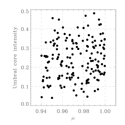
Figure 18: Umbral core intensity versus $\mu$ for all spots with umbral radii between 5 arc-sec and 15 arc-sec.

Figure 19: Umbral core intensity (a) and umbral radius (b) versus time since solar cycle minimum for Northern (filled circles) and Southern (asterisks) hemispheres, for all observed sunspots. Each plotted symbol represents an average over 10 sunspots. The solid and dashed lines show the linear regression fits for Northern and Southern hemispheres, respectively. The best linear fits are given in the lower left corner.

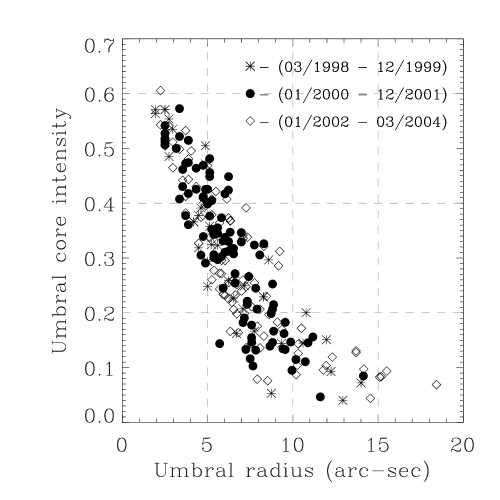
Figure 20: Umbral core intensity versus umbral radius. Different symbols represent spots observed in ascending, maximum and descending phases of solar cycle. The dates indicate the period of observation.

In Figs. 15(a) and (b) we display the umbral core intensity for two different umbral size ranges, i.e. for spots with umbral radii in the range 5″ - 10″ and in 10″ - 15″, respectively. The trend seen here is opposite for small and large spots, but is insignificant in both cases (see column Gradient/$\sigma$ in Table 3). If we plot all the sunspots, irrespective of radius, the results are not significantly different.

In Figs. 16(a) and (b) we plot the dependence on the time elapsed from activity minimum, of the analysed sunspot umbral radius, separately for the small (5″ - 10″) and the large (10″ - 15″) spots, respectively. The linear regression are overplotted. The mean umbral radius of the analysed spots between 5″ - 10″ slightly decreases with time, whereas spots with radius between 10″ - 15″ show the opposite trend. Similarly in Fig. 1 the umbral radii of all studied spots are plotted. The regression parameters for the full sample of spots (5″ - 10″) is given in Table 3. Although none of these trends is statistically significant, they are opposite to the trends (also not statistically significant) shown by the umbral brightness of these spots. This is completely consistent with the dependence of brightness on umbral radius shown in Figs. 10 - 12.

Another bias can be introduced by the fact that the sunspot latitude systematically decrease over a solar cycle. We have to a certain extent reduced this effect by considering only sunspots at $\mu>0.94$. Figure 17 shows the average $\mu$ of the analysed sunspots, as expected, this displays an increase over the cycle. In order to judge whether this introduces a bias into the cycle phase dependence of sunspot brightness we plot in Fig. 18 umbral core brightness (i.e. contrast to local quiet Sun) versus $\mu$ (for $0.94<\mu<1$). We did not find any significant variation in the umbral core brightness with $\mu$.

In order to check for an asymmetry in umbral brightness between the northern and southern hemispheres as reported by Norton & Gilman (norton (2004)), in Fig. 19 we plot umbral core brightness separately for northern and southern hemispheres. In this plot we used corrected intensities for all the observed spots. The intensities are binned and each bin contains 10 samples. The linear regression fit provides a slightly higher gradient in the northern hemisphere. But this can be well explained by the increase in umbral radius of the spots with the cycle phase (Fig. 19(b)). It should be noted that Norton & Gilman observed a significant umbral brightness difference between the northern and southern hemisphere during the onset of cycle 23. Due to the restriction of $0.94<\mu$ in our selection criteria, we have analysed only few spots during this period and hence cannot comment on that result.

In Table 3 we also list the parameters of the linear regressions to mean umbral and penumbral intensities versus time. None of the gradients is significant at even the 1$\sigma$ level. Also, the signs of the gradients of all umbral core and mean intensity samples are opposite to those of the umbral radius of the corresponding sample, suggesting that even any small gradient in the umbral brightness is due to a small bias in the umbral size with time. Hence we find no evidence at all for a change in sunspot brightness over the solar cycle.

In order to test whether the dependence of umbral core brightness on umbral radius in Sect. 4.1 is itself dependent on solar cycle phase we plot in Fig. 20 the umbral core brightness versus radius but now for three different phases of the cycle. Asterisks, filled circles and diamond symbols represent the spots observed in ascending, maximum and descending phases of solar cycle, respectively. As can be clearly seen there is no difference between the different phases. This demonstrates that there is no cross-talk between cycle phase dependence and umbral radius dependence of umbral brightness.

6 Discussion

With a large sample of sunspots, we have tested if the umbral core brightness, the umbral average brightness, or the penumbral brightness depend on solar cycle phase. In addition to this, we studied the dependence of brightness on sunspot size.

Earlier continuum observations suggested that large sunspots are darker than smaller sunspots (Bray & Loughhead bray (1964)). But most of such observations were barely corrected for stray light (Zwaan zwaan (1965)). Subsequent observations which were corrected for stray light showed no significant dependence of umbral core brightness on spot size (Albregtsen & Maltby albregtsen2 (1981)). More recent observations however, reveal that even after stray-light correction a size dependence remains. Thus, Kopp & Rabin (kopp (1992)) present observations at 1.56 ${\rm{\mu m}}$ that show clear evidence for the size dependence of umbral brightness. Also, results from two sunspots observed at the same wavelength combined with the Kopp & Rabin data confirm and strengthen the linear dependence of brightness on sunspot umbral size (Solanki solanki1997 (1997), Solanki et al. solanki1 (1992), Kopp & Rabin kopp (1992), R$\mathrm{\ddot{u}}$edi et al. ruedi (1995)).

Martínez Pillet & V$\acute{\rm a}$zquez (martinez (1993)) confirmed the Kopp & Rabin result based on the analysis of 7 sunspots. Collados et al. (collados (1994)) found from the inversion of Stokes profiles obtained in 3 sunspot umbrae that small umbrae are distinctly hotter than large umbrae. One disadvantage of all these studies is that each is restricted to a relatively small number of sunspots. Another is that each sunspot was observed under different seeing conditions, so that the level of stray light varied in an unsystematic manner. Both shortcomings are addressed in the present paper.

In our analysis we found a clear dependence of umbral core brightness on umbral size. Since we correct for the very slowly varying stray light and the MDI specific problem of cross-talk of the spectral line into the continuum, as described in Sect. 3 and the appendix, our results are basically free from stray light contamination. This is particularly true for umbral core intensities as we could show using the Mercury transit data. For mean intensities some residual remains (see Appendix A). Also, we have a relatively large sample of sunspots to support our results. We carried out and compared two different fits to the umbral brightness-size dependence for the analysed spots, a double linear fit for two different umbral size ranges and a power law fit to the entire data set. A similar analysis of umbral brightness and diameter carried out at a wavelength of 1.56 $\rm\mu m$ (Solanki solanki1997 (1997)) shows a smaller gradient than what we obtained in our work. Umbral brightness for 9 spots, with umbral diameter ranging from 5″ to 35″ were included in the above study. From a linear fit, a gradient of around $-0.012/\arcsec$ is obtained for the umbral brightness, whereas in our case a much higher gradient of $-0.04/\arcsec$ is found. This is not surprising since the brightness at 1.56 $\rm\mu m$ reacts much more weakly to a given temperature change than at 677 $\rm{nm}$.

Albregtsen & Maltby (albregtsen1 (1978)) reported a variation of umbral core brightness with solar cycle by analysing 13 sunspots. The results were mainly presented for the observations done at a wavelength of 1.67$\rm{\mu m}$. They found an increase in umbral core intensity by as much as 0.15 from early to late phase of the solar cycle. They also found no dependence of umbral brightness on other sunspot parameters, such as size and type of the spot. In a later paper Maltby et al. (maltby (1986)) detailed this variation for a range of wavelengths starting from 0.38 - 2.35 $\rm{\mu m}$. The nearest wavelength to our observations (i.e. 0.669 $\rm{\mu m}$) shows a variation of around 0.072 in umbral core intensity from early to late phase, this corresponds to 0.0065 umbral intensity variation per year. Based on these findings they presented three different umbral core model atmospheres for sunspots present in the early, mid and late phase of the solar cycle. In a recent study carried out using MDI data Norton & Gilman (norton (2004)) find a relatively smooth decrease in the umbral brightness from activity minimum to maximum for Northern hemisphere and no distinct trend for the southern hemisphere. The decrease in umbral brightness with solar cycle they found is opposite to the results of Maltby et al. (maltby (1986)).

In our analysis we found a very feeble, statistically insignificant dependence of umbral brightness on solar cycle (i.e. any change remains well within the error bars). The linear fit to umbral core brightness is given by the following equation,

$$I_{uc}=0.222+(0.004\pm 0.006)\times t$$ (1)

where $t$ is the time elapsed from the minimum in units of years. All sunspots within 5″ - 15″ umbral radius are included in the regression. It is striking that the 1$\sigma$ uncertainty in the gradient obtained in our analysis is approximately equal to the trend found by Maltby et al. (maltby (1986)). Therefore, either the MDI wavelength is less suitable than the 1.56 $\rm\mu m$ wavelength band employed by Maltby and co-workers, or there is a selection bias affecting their results. Indeed, the change in umbral core intensity over the solar cycle reported by Maltby et al. (maltby (1986)), 0.072, is only $1/3$ the umbral core intensity difference between spots with umbral radii of 5″ and 15″ found here and is 0.6 times the intensity difference between such spots at 1.56 $\rm\mu m$. Consequently, selection biases, which often afflict small samples, can introduce an artificial trend of the correct magnitude over an activity cycle.

In order to reduce the effect of size dependence on the above relation, we grouped the sunspots into two umbral radii bins. The linear regressions to these groups are given by the following equations,

$$I_{uc}=\{\begin{array}[]{ll}0.250+(0.002\pm 0.006)\times t&{\rm for}\leavevmode\nobreak\ \leavevmode\nobreak\ 5^{\prime\prime}-10^{\prime\prime}\\ 0.126-(0.003\pm 0.005)\times t&{\rm for}\leavevmode\nobreak\ \leavevmode\nobreak\ 10^{\prime\prime}-15^{\prime\prime}\end{array}$$ (4)

For the group of spots with umbral radii between 5″ - 10″ the linear regression fit gives an increase in umbral brightness with increasing phase of the solar cycle, but again the change is within the error bars. For the spots with umbral radii 10″ - 15″ the opposite trend is found. We compared these results with the variation of the sizes of the analysed sunspots over the solar cycle. It turns out that for all three samples (5″- 10″, 10″-15″, 5″-15″) the average radii show the opposite trend to the intensity. This suggests that at least part of any trend in brightness over the solar cycle is due to a corresponding (opposite) trend in umbral radii.

From these results it is evident that the dependence of the brightness of the spot on size is an important parameter to be considered when the umbral brightness variation with solar cycle is studied. We believe that without showing the time dependence of the average area or size of the sunspot umbrae in the employed samples, any studies of sunspot brightness (or even field strength) evolution over time are of limited value. Although there is no systematic variation in the relative distribution of umbral areas with solar cycle (Bogdan et al. bogdan (1988)) in a smaller sunspot sample a trend may be introduced by limited statistics. It would therefore be of great value to determine the areas of the umbrae studied by Penn & Livingston (penn (2006)), who find a steady decrease of the maximum umbral field strength over the last 7 years, since the field strength is related to brightness (Maltby maltby2 (1977), Kopp & Rabin kopp (1992), Martínez Pillet & V$\acute{\rm a}$zquez martinez (1993), Solanki et al. sol1993 (1993), Mathew et al. mathew2004 (2004), Livingston livingston (2002)), which depends on size (Sect. 4.1). Also, our results imply that models of the umbral atmosphere (e.g. Avrett avrett (1981), Maltby et al. maltby (1986), Caccin et al. caccin (1993), Severino et al. severino (1994), Fontenla et al. fontenla (2006)) should always indicate the spot size to which they refer.

Chapman et al. (chapman (1994)) reported photometric observations of sunspot groups, that show considerable variation in their mean contrast. This could be due to umbra/penumbra area ratio change, or due to intrinsic brightness change. Our results suggest that, at least in part the later is the reason. This has implications for irradiance reconstructions, particularly those using separate atmospheric components for umbrae and penumbrae (e.g. Fligge et al. fligge (2000), Krivova et al. krivova (2003)).

The result is also of importance for the physics of sunspots, since an explanation must be found why a smaller heat flux is transported through the umbrae of larger sunspots. E. g. in Parker’s (parker (1979)) spaghetti model it would imply that either the filamentation of the subsurface field is less efficient under larger umbrae, or that the energy flux transported between the filaments is smaller for larger filaments. One factor which probably plays a role is that darker sunspots have higher field strengths (Maltby maltby2 (1977), Kopp & Rabin kopp (1992), Livingston livingston (2002)) which are more efficient at blocking magnetoconvection. This also implies that larger sunspots have stronger fields.

The only clear dependence we have found in our sample of sunspots is between umbral intensity and radius. However, even this relationship shows considerable scatter, whose origin is not clear. We list some possibilities below:

1. dependence of the scattered light correction on the shape of the umbra (e.g. very elongated versus circular);

2. dependence of intrinsic brightness of umbrae on shape and complexity;

3. dependence of brightness on age;

4. (small) dependence of brightness on phase of the solar cycle;

5. CLV of umbral contrast (which is small according to Fig. 18).

Separating clearly between these possibilities is beyond the scope of the current paper. Our analysis is restricted to regular sunspots with single umbrae. Complex spots may in principle show a different behaviour.

7 Concluding remarks

In this paper we present the analysis of MDI continuum sunspot images aimed at detecting umbral core brightness variation with solar cycle. We analysed a total of 234 sunspots of which 164 sunspots have an umbral radius lying between 5″ - 15″. Careful corrections for stray light and the Zeeman splitting of the nearby Ni I line on measured continuum intensities have been made. We derive the following conclusions from our analysis.

• The umbral core and mean brightness decreases substantially with increasing umbral radius.

• The mean penumbral intensity is also reduced with increased spot size, but by a small amount.

• No significant variation in umbral core, umbral mean and mean penumbral intensities is found with solar cycle.

• The insignificant variation with solar cycle of the umbral intensity could be at least partly be explained by the dependence of the analysed spot size on solar cycle.

Appendix A Stray-light evaluation and image restoration of MDI data

The point spread function used to fit the limb profiles follows Martínez Pillet (valentin (1992)) and it includes three Gaussians and one Lorentzian component:

Figure 21: Dependence between umbral intensity and size (a) used to compute the contamination levels (observed intensity minus true intensity) shown in (b). Solid lines correspond to a constant umbral intensity for all umbral sizes. Dashed lines correspond to a linear decrease of umbral intensity with umbral radius. Dashed-dot lines represent a combination of the two previous cases. The spread functions used are those derived from the Mercury transit observations.

$$\psi(r)=\sum_{i=1}^{3}m_{i}a_{i}exp(-{{r^{2}}\over{b_{i}^{2}}})+M{{A}\over{B^{2}+r^{2}}}{\bf,}$$ (5)

where $r$ is the radial distance from disk centre, $m_{i}$ and $M$ the weights of the different components (that add to 1), $b_{i}$ the corresponding Gaussian parameters, $B$ the Lorentzian parameter and $a_{i}$ and $A$ the normalisation constants (see Martínez Pillet valentin (1992), equations 23 and 24). The theoretical CLV used for the (two-dimensional) convolution with the spread function is a simple polynomial:

$${{I(r)}\over{I_{0}}}=\sum_{i=1}^{6}c_{i}\mu^{i}(i-1){\bf,}$$ (6)

with $\mu$ the cosine of the heliocentric angle. Note that all polynomial coefficients, $c_{i}$, add to one. The azimuthally averaged MDI continuum intensity profiles are fitted with a standard non-linear least-squares algorithm. The free parameters are the Gaussian and Lorentzian parameters ($b_{i}$ and $B$), the three Gaussian weighting parameters ($m_{i}$) and five of the CLV coefficients ($c_{i}$). In total there are 12 free parameters. While we originally left fixed the CLV coefficients to values found in the literature, it was clear from the residuals observed inside the solar disk that they should be left also as free parameters (note also that the continuum of MDI does not correspond to a clean continuum, as explained in the text).

In Table A.1, we provide the spread function fitted parameters for four frames observed during the Mercury transit on the 7th of May, 2003. The corresponding limb profiles were all very similar and showed differences at the few $10^{-4}$ level (of the disk centre intensity). The only parameter that changes more considerably is the Lorentzian parameter $B$, but we note that this procedure to fit the stray-light is known to be very insensitive to this parameter (see Martínez Pillet valentin (1992)). The stray-light levels far away from the solar limb are known to be more closely linked to the values of the Lorentzian weighting parameter $M$. Indeed, it is a change in this parameter from $M=0.116$ in 1996 to $M=0.17$ in 2003 that explains the steady increase in scattered light in the MDI instrument seen in Fig. 3.

Table 4: Spread function parameters from Mercury transit data

Parameter	Frame 1 UT 07:59:30	Frame 2 UT 09:35:30	Frame 3 UT 11:11:30	Frame 4 UT 12:47:30
$b_{1}$ (″)	2	2	2	2
$b_{2}$ (″)	6	6	6	6
$b_{3}$ (″)	18	17	16	17
$B$ (″)	61	47	40	46
$m_{1}$	0.676	0.672	0.693	0.694
$m_{2}$	0.117	0.123	0.108	0.107
$m_{3}$	0.035	0.033	0.029	0.029
$M$	0.173	0.171	0.170	0.171

The first Gaussian, with a 2″ parameter (FWHM 3.5″), represents the pixel dominated MDI resolution. The other Gaussian and Lorentzian terms represent contributions from diffraction and scattering by the optical components. Umbral scattered light is dominated by the widest Gaussian ($b_{3}$, of around 30″ FWHM) and the Lorentzian components.

Once the spread function is derived for a given image, we proceed with its restoration. If $O(u,v)$ is the Fourier transform of the observed image, the restored image is computed as the inverse Fourier transform of $O^{R}(u,v)$, defined as follows:

$$O^{R}(u,v)=O(u,v)\Phi(q)T(q)$$ (7)

with $q=\sqrt{u^{2}+v^{2}}$ the radial coordinate in the Fourier domain. $\Phi(q)$ corresponds to the division by the Fourier transform of the spread function, $t(q)$ (the modulation transfer function), defined within the optimum filter scheme. That is:

$$\Phi(q)={{t(q)}\over{t^{2}(q)+{{1}\over{SNR^{2}(q)}}}}$$ (8)

with $SNR(q)$ the Signal-to-Noise Ratio of the data in the Fourier domain. The level of white noise used for this quantity was estimated, as usual, by observing the high frequency part of the power spectrum of the data. Finally, $T(q)$ is a cosine based apodization window whose effect is to reduce the restoration of the intermediate Gaussian component and completely avoid any restoration from the Gaussian component corresponding to the pixel sampling. The apodization window leaves the restoration of the Lorentzian and broadest Gaussian component almost untouched. The exact level of apodization (48%) was fine tuned by using the Mercury observations. If a full restoration is used with no apodization window, umbral intensities remain within 1-2 percent of their value obtained with apodization, but Gibbs oscillations are enhanced at the limb in the restored data. These Gibbs oscillations also affect our penumbral intensities for the smallest spots and our apodization function helps to minimise their effect.

The restoration in the Fourier domain is made with images that are twice as large as the original MDI images (i.e. 2048$\times$2048 frames). Only when these extended images were used, could we recover a clean zero intensity value (in the restored frames) beyond the solar limb (see Fig. 4). Restoration using normal size frames always produced negative values in this area. The reason for this behaviour was found to be the doubled sampling in the Fourier domain of the transform of the Lorentzian component. This component, being the most extended one, has a very sharp peak at low frequencies in the MTF. This peak was correctly sampled only when the extended images were used. The stray light was artificially prolongated in the extended observed images using the fitted spread function parameters.

The observed core intensity of Mercury (12″ diameter) is 0.16 of the surrounding photosphere and the mean value over the planet’s disk 0.23. After the restoration the core intensity is $-0.02$ (slight over correction) and the mean value 0.09. This shows that our restoration provides core intensities that are correct to within a few percent and mean values that are under corrected by 10% for pores that are of a size similar to Mercury. Sunspots of this size or larger will have much better accuracies in both core and mean intensities.

A visual inspection of Fig. 10 shows that the correction applied by our algorithm turns out to be larger for larger sunspots and becomes smaller for the smallest ones. At first sight this result is somewhat puzzling. One expects smaller spots to show larger contamination levels (defined as observed minus corrected intensities), but we caution that this is only true as long as the intrinsic brightness of the spots remains the same for different sizes. A correlation between sunspot size and continuum intensity (as found in this paper, i.e. increase in intensity with decreasing size) can mask this trend. To confirm that for small bright sunspots one can expect lower contamination levels, we performed simulations where a brightness-size relationship was assumed and estimated the contamination levels using the spread functions derived for the MDI instrument during the Mercury transit. The simulations consist of locating a sunspot of a known size and brightness at the centre of an artificial solar image that displays the CLV derived from our analysis. These images are convolved (also with 2048$\times$2048 frames) with the inferred spread function and the contamination level for this sunspot size is directly evaluated from the convolved image. The results can be seen in Fig. A.1. Three cases are presented, umbral intensity constant for all sizes (solid line), a linear decrease of umbral intensities with umbral radii (dashed line) and, finally, a steeper linear decrease for smaller umbrae with radii less than 8.6″and a constant intensity value for larger umbrae (dot-dashed line). The contamination levels obtained from the first case (constant intensity) show the expected result of monotonically decreasing values for larger umbrae (solid line). When the umbral intensity is smaller for larger umbrae (dashed line), the contamination level initially shows the same tendency of smaller levels for larger sunspots but soon changes the slope and provides a larger contamination for larger sunspots. The third case shows that when there is a very strong dependence between umbral intensities and sunspot sizes (smaller spots are brighter) the contamination levels are always larger for larger sunspots. This tendency is reversed when the umbral intensities remain constant for the largest sunspots. Then, the expected decrease of the contamination levels for larger umbrae is found again. The shape of this (dot-dashed) curve is reminiscent of the dependence between the observed contamination levels and umbral sizes shown in Fig. 10. We thus conclude that the observed increased brightness for smaller sunspots in this Figure is perfectly compatible with stray light corrected data and reflects a real tendency of solar spots.

References

- (1) Albregtsen, F., Maltby, P. 1978, Nature, 274, 41
- (2) Albregtsen, F., Maltby, P. 1981, Sol. Phys., 71, 269
- (3) Albregtsen, F., Jorås, P. B., Maltby, P. 1984, Sol. Phys., 90, 17
- (4) Avrett, E. H. 1981, in The Physics of Sunspots, L. E. Cram, J. H. Thomas (Eds.), National Solar Obs., Sunspot, NM, p. 235
- (5) Bogdan, T. J., Gilman, P. A., Lerche, I., Howard, R. 1988, ApJ, 327, 451
- (6) Bray, R. J., Loughhead, R. E. 1964, Sunspots, Chapman and Hall, London
- (7) Caccin, B., Gomez, M. T., Severino, G. 1993, A&A, 276, 219
- (8) Chapman, A. G., Cookson, S. M., Dobias, J. J. 1994, ApJ, 432, 403
- (9) Collados, M., Martínez Pillet, V., Ruiz Cobo, B., del Toro Iniesta, J. C., Vzquez, M. 1994, A&A, 291, 622
- (10) Fligge, M., Solanki, S. K., Unruh, Y. C. 2000, A&A, 353, 380
- (11) Fontenla, J. M., Avrett, E., Thuillier, G., Harder, J. 2006, ApJ, 639, 441
- (12) Grevesse, N., Sauval, A. J. 1998, Space Sci. Rev., 85, 161
- (13) Kopp, G., Rabin, D. 1992, Sol. Phys., 141, 253
- (14) Krivova, N. A., Solanki, S. K., Fligge, M., Unruh, Y. C. 2003, A&A, 399, L1
- (15) Kurucz, R. L., Furenlid, I., Brault, J. W. 1984, Solar flux atlas from 296 to 1300 nm, National Solar Observatory Atlas, Sunspot, New Mexico
- (16) Kurucz, R. L., 1991, in Stellar Atmospheres: Beyond Classical Models, L. Crivellari, I. Hubeny, D. G. Hummer (Eds.), NATO ASI Series, Kluwer, Dordrecht, p.440
- (17) Livingston, W. 2002, Sol. Phys., 207, 41
- (18) Maltby, P. 1977, Sol. Phys., 55, 335
- (19) Maltby, P., Avrett, E. H., Carlsson, M., Kjeldseth-Moe, O., Kurucz, R. L., Loeser, R. 1986, ApJ, 306, 284
- (20) Martínez Pillet, V. 1992, Sol. Phys., 140, 207
- (21) Martínez Pillet, V., Vzquez, M. 1993, A&A, 270, 494
- (22) Mathew, S. K., Solanki, S. K., Lagg, A., Collados, M., Berdyugina, S., Frutiger, C., Krupp, N., Woch, J., 2002, in Poster Proc. 1st, Potsdam Thinkshop on Sunspots and Starsspots, K. G. Strasmeier, A. Washuettl (Eds.), AIP, p. 117
- (23) Mathew, S. K., Solanki, S. K., Lagg, A., Collados, M., Borrero, J. M., Berdyugina, S. 2004, A&A, 422, 693
- (24) Norton, A. A., Gilman, P. A. 2004, ApJ, 603, 348
- (25) Ortiz, A., Domingo, V., Sanahuja, B. 2006, A&A, 452, 311
- (26) Parker, E. N. 1979, ApJ, 230, 905
- (27) Penn, M. J., Livinston, W. 2006, ApJ, 649, L48
- (28) Pettauer, T., Brandt, P. N. 1997, Sol. Phys., 175, 197
- (29) Pierce, A. K., Slaughter, C. D. 1977, Sol. Phys., 51, 25
- (30) Redi, I., Solanki S.K., Livingston W. 1995, A&A, 302, 543
- (31) Scherrer, P. H., Bogart, R. S., Bush, R. I., et al. 1995, Sol. Phys., 162, 129
- (32) Schssler, M. 1980, Nature, 288, 150
- (33) Severino, G., Gomez, M. T., Caccin, B. 1994, in Solar surface magnetism,, R. J. Rutten, C. J. Schrijver (Eds.), Kluwer, Dordrecht, p. 169
- (34) Solanki, S. K. 1997, in Advances in the Physics of Sunspots, B. Schmieder, J. C. del Toro Iniesta, M. Vzquez (Eds.), Astron. Soc. Pacific Conf. Ser., Vol. 118, p.178
- (35) Solanki, S. K. 2003, A&A Rev., 11, 153
- (36) Solanki, S. K., Redi, I., Livingston, W. 1992, A&A, 263, 339
- (37) Solanki S. K., Walther, U., Livingston W. 1993, A&A, 277, 639
- (38) Unruh, Y. C., Solanki S. K., Fligge, M. 1999, A&A, 345, 635
- (39) Walton, S. R., Preminger, D.G. 1999, ApJ, 514, 959
- (40) Yoshimura, H. 1983, Sol. Phys., 87, 251
- (41) Zwaan, C., 1965, in Proceedings of the IAU Symposium no. 22, R. Lst (Ed.), p.277