A Systematic Search for High Surface Brightness Giant Arcs in a Sloan Digital Sky Survey Cluster Sample

Abstract

We present the results of a search for gravitationally-lensed giant arcs conducted on a sample of 825 SDSS galaxy clusters. Both a visual inspection of the images and an automated search were performed and no arcs were found. This result is used to set an upper limit on the arc probability per cluster. We present selection functions for our survey, in the form of arc detection efficiency curves plotted as functions of arc parameters, both for the visual inspection and the automated search. The selection function is such that we are sensitive only to long, high surface brightness arcs with $g$-band surface brightness $\mu_{g}\leq 24.8$ and length-to-width ratio $l/w\geq 10$. Our upper limits on the arc probability are compatible with previous arc searches. Lastly, we report on a serendipitous discovery of a giant arc in the SDSS data, known inside the SDSS Collaboration as Hall’s arc.

1 Introduction

Clusters of galaxies are the largest gravitationally bound structures in the universe. It has long been recognized that they constitute very usefeul probes for cosmology (see, e.g., Press & Schechter, 1974; Mohr et al., 2001; Voit, 2005), and therefore understanding them in detail has been a major field of research. Notable progress in the theoretical understanding of clusters has been achieved in recent years through N-body and hydrodynamical simulations. At present, different simulation schemes converge in reproducing several broad properties of clusters (Frenk et al., 1999; Heitman et al., 2005). Furthermore, several properties of the simulated clusters are in agreement with observations (see, e.g., Borgani et al., 2004; Evrard et al., 2002; Eke et al., 1998).

The strong gravitational lensing of background galaxies produced by massive clusters is a probe of cluster structure. This effect has been observed in many previous studies, with the most extreme case being the giant gravitational arcs first seen by Lynds & Petrosian (1989) and Soucail et al. (1987). Almost a decade later, spectacular images of these arcs were provided by the excellent resolution of the Hubble Space Telescope (Couch & Ellis, 1995; Kneib et al., 1996; Smail et al., 1996). There are now about a hundred clusters with giant arcs imaged by HST (for a recent compilation, see Sand et al., 2005). Several arc searches have been carried out with ground based observations, both for X-ray selected clusters (see, e.g., Luppino et al., 1999; Cypriano, 2002; Campusano et al., 2006) as well as for optically identified clusters (Zaritsky & Gonzalez, 2003; Gladders et al., 2003).

The comparison of the abundance of gravitational arcs with theoretical predictions has been proposed as a tool to constrain cosmology (Grossman & Narayan, 1988; Miralda-Escudé, 1993; Wu & Hammer, 1993). The early results indicated that the number of strongly-lensed arcs greatly exceeded that expected from $\Lambda$CDM simulations (Bartelmann et al., 1998). More detailed studies of the theoretical uncertainties and systematic effects involved in this analysis seem to indicate that the observations do, in fact, agree with the theoretical expectations from the standard cosmology (Hennawi et al., 2005; Dalal et al., 2004; Wambsganss et al., 2004; Oguri et al., 2003), although uncertainties may still remain (Li et al., 2005).

The main goal of the work presented here is not in the extraction of cosmological information from the statistics of gravitational arcs. Instead it is both (a) to locate high surface brightness giant arcs that would prove useful in follow-up imaging and spectroscopy programs, and more directly (b) to understand the probability for a galaxy cluster to produce a giant arc as a function of the cluster mass and redshift. We believe this is an important aspect to be considered before cosmology can be extracted from arc statistics and that it will provide a significant improvement in our understanding of the mass distribution inside galaxy clusters.

A defining characteristic of previous arc searches is that they were done in the most massive clusters. Luppino et al. (1999) searched for arcs in 38 X-ray selected clusters (redshifts $0.15\leq z\leq 0.82$) with X-ray luminosity $L_{x}\geq 2\times 10^{44}$ ergs/sec and found arcs in a high fraction of clusters with $L_{x}>10^{45}$ ergs/sec, but no arcs in clusters with $L_{x}<4\times 10^{44}$ ergs/sec. Zaritsky & Gonzalez (2003) searched for arcs in 44 optically selected clusters ($0.5\leq z\leq 0.8$) from a list ranked by surface brightness, finding arcs in two clusters. Gladders et al. (2003) searched $\approx 900$ optically selected clusters ($0.3\leq z\leq 1.4$) ranked by a galaxy overdensity parameter, finding arcs in 8 clusters, with none at $z<0.64$. Sand et al. (2005) used a very different technique, searching for arcs in the heterogeneous sample of clusters that have been observed with HST; out of 128 clusters ($0.1\leq z\leq 0.78$) 45 had tangential arcs, although it is worth noting that many of the clusters were targeted by HST precisely because of known arcs.

It is possible to compute which of the arcs found in high quality images would be found in images of lower quality, and we will perform such a comparison. The results so far suggest looking for arcs in clusters with high X-ray luminosity or high redshift. Luppino et al. (1999) found a higher frequency of arcs in high $L_{x}$ clusters, and since the bremstrahlung emission in clusters is proportional to $n_{e}^{2}$, this result suggests that arcs are found preferentially in the highest density clusters. Gladders et al. (2003) found a higher frequency of arcs in higher redshift clusters, which suggests either an evolution of cluster structure in a way not fully understood, or perhaps that the sources lensed are predominately at higher redshifts, where the lensing cross section would be much larger for $z\sim 0.7$ clusters than for those at $z\sim 0.3$ (Ho & White, 2005). Observationally, however, it is clear that the dominant variables for successful arc detection are limiting surface brightness and, in particular, seeing.

The Sloan Digital Sky Survey (York et al., 2000) to date has produced multiband $ugriz$ imaging of $8000$ deg² of the northern sky, along with an associated catalog of 1,048,496 spectra, of which 674,749 are galaxies (Adelman-McCarthy et al., 2006). It has proven useful as a data set for gravitational lens searches. An example is the multiply-lensed quasar searches of Pindor et al. (2003) and Oguri et al. (2006), which use the imaging data to select quasar-colored objects that are larger than a PSF, or groupings of quasar-colored objects in a small area. A second example of lens searches in the SDSS data uses the large SDSS spectroscopic data set: Bolton et al. (2006) searched red galaxy spectra for indications of a second, higher redshift nebular emission spectrum. This locates strongly-lensed background galaxies, which are revealed as arcs after applying galaxy subtraction techniques on HST ACS images. Our program is a search for strongly-lensed background galaxies behind clusters; that is, a search for giant arcs. Our ability to locate gravitational arcs in the SDSS images is demonstrated by recovering arcs observed by other surveys and by the discovery of new gravitational arcs (see Fig. 1, Appendix A, and Allam et al., 2006). A similar arc search in a sample of 240 rich SDSS clusters has been carried out by Hennawi et al. (2006) and has found a significant number of new giant arc systems, but relies on deeper imaging data to discover the arcs, whereas we use the original SDSS imaging data itself.

Our analysis consists of a search for giant gravitational arcs in a sample of SDSS galaxy clusters sorted by a richness estimator. Our imaging data does not have the depth or seeing available to previous searches, but it does have the twin features of homogenity and large sky coverage. This results in our ability to greatly increase the number of clusters searched. The search reported here totals 825 clusters, comparable to the largest previous search. We intend, in a future paper, to decrease the mass threshold down to the poor group range in order to search tens or hundreds of thousands of locations. Furthermore, the redshift range of the cluster catalog we have searched is predominantly $0.1\leq z\leq 0.3$, a regime poorly covered by previous searches.

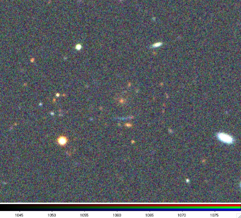
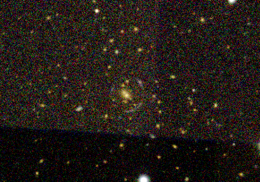
Figure 1: On the left, the SDSS image of the RCS1419.2+5361 cluster. The arc was discovered by visual inspection of the RCS cluster sample (Gladders et al., 2003) and is clearly visible in this color image composed of the SDSS $g$, $r$, and $i$ data. On the right, Hall’s arc (see Appendix), serendipitously discovered in the SDSS data. It too is clearly visible in the composite $gri$ image. These observations, together with the recent discovery of a new arc system (Allam et al., 2006), demonstrate the ability of the SDSS to detect high surface brightness giant arcs.

2 The Data

The data set we use is the Sloan Digital Sky Survey (SDSS) Data Release 5 (DR5; Adelman-McCarthy et al., 2006). The SDSS uses a wide-field drift-scanning mosaic CCD camera (Gunn et al., 1998) on a dedicated 2.5m telescope (Gunn et al., 2006) at Apache Point Observatory, New Mexico, to image the sky in the five photometric bandpasses $ugriz$ (Fukugita et al., 1996; Stoughton et al., 2002). The SDSS photometric data are processed using pipelines that address astrometric calibrations (Pier et al., 2003), photometric data reduction (Lupton et al., 2001), and photometric calibrations (Tucker et al., 2006; Smith et al., 2002; Hogg et al., 2001; Ivezic et al., 2004). Note that the SDSS is a survey that trades relatively shallow exposures – 55 seconds on a 2.5m telescope, resulting in point sources detected at $95\%$ confidence level at $g=22.2$ and $i=21.3$ (AB) – for a very wide area: 8000 deg² or $20\%$ of the total sky.

2.1 The Cluster Sample

The cluster catalog was constructed using the maxBCG algorithm. This is a red-sequence locating technique that has shown completeness levels of $90\%$ at $0.1\leq z\leq 0.3$ and down to $N_{g}=10$, where $N_{g}$ is the number of galaxies on the E/S0 red sequence brighter than $0.4L^{\star}$ and within $1h^{-1}$ Mpc of the brightest cluster galaxy. The correlation of the richness $N_{g}$ with mass can be calibrated with independent mass estimators, such as velocity dispersions or weak lensing shear profiles. A detailed description of the maxBCG technique is discussed in Koester et al. (2006a). Koester et al (2006b) used the SDSS DR5 data to construct a cluster catalog containing 12,875 rich clusters, plus two orders of magnitude more clusters of lower masses. The catalog we used in this work was created using an earlier version of the maxBCG algorithm (see, e.g., Hansen et al., 2005; Sheldon et al., 2001).

One of the defining features of red sequence methods is that projection effects are present only at a minimal level: if the clusters differ by $\Delta z<0.05$ then they can be confused as a single object. The resulting purity (lack of false positives) is $\approx 95\%$, and the completeness (lack of false negatives) is $\approx 85\%$ above $1\times 10^{14}M_{\sun}$, as determined by running this algorithm on mock catalogs (Koester et al, 2006b).

We selected a sample of 825 clusters with $N_{g}\geq 20$, approximately 50% of the $N_{g}\geq 20$ clusters in our sample. The whole sample was not searched due to a variety of technical reasons, but lack of a complete sample is not important for the results of this paper. The distribution of $g$-band seeing of the cluster images is shown in Fig. 2 and has a mean of $1.44^{\prime\prime}$; this is important because the seeing is the single dominating factor in our ability to detect arcs. The cluster redshift distribution is shown in Fig. 3. The richest clusters in our sample are presented in Table LABEL:clusterlist, and the table listing our full cluster sample is available electronically.

Figure 2: The $g$-band seeing distribution for the SDSS images of the 825 clusters inspected in this paper. The distribution is well fit by a gaussian of mean 1.44” and standard deviation 0.20”.

Figure 3: The redshift distribution for the 825 clusters inspected for this paper. We have good statistics in the redshift range $0.1<z<0.3$.

While we do not use the masses of the clusters directly in this work, we do have a rough mass calibration. Stacked cluster spectroscopic velocity dispersions, plus isothermal sphere fits to stacked cluster weak lensing shear profiles, both from early work in the SDSS EDR (see, e.g. Bahcall et al., 2003; Sheldon et al., 2001), were combined to produce a scaling relation between velocity dispersion $\sigma_{v}$ and $N_{g}$ given by $\sigma_{v}\approx 85N_{g}^{0.6}$ km/s. Modeling the cluster as a singular isothermal sphere, the mass enclosed within a radius having an overdensity of 200 with respect to the critical density is (see, e.g. Bryan & Norman, 1998)

$$M_{200}=\Big{(}\frac{\sigma_{v}}{\sigma_{0}}\Big{)}^{3}\frac{1}{E(z)h}\quad 10^{15}M_{\sun},$$ (1)

where $\sigma_{0}=1148$ km/s, $E(z)=\sqrt{\Omega_{\Lambda}+\Omega_{m}(1+z)^{3}+(1-\Omega_{\Lambda}-\Omega_{m})(1+z)^{3}}$, $h$ is the Hubble constant in units of 100 km/s/Mpc, and $\Omega_{m}$ and $\Omega_{\Lambda}$ are the energy densities of cold/presureless normal matter and the cosmological constant, respectively, in units of the critical density. The $\sigma_{v}$-$N_{g}$ relation has a significant scatter. Indirect methods, such as (a) running the cluster finding algorithm on mock catalogs based on N-body simulations and (b) measuring the higher moments of the velocity distributions of galaxies in stacked cluster samples, suggest that the scatter is $\Delta M_{200}/M_{200}\sim 40\%$ at high $N_{g}$ and increases at lower $N_{g}$. A more sophisticated calibration using weak lensing measurements of the full maxBCG catalog is given in Sheldon (2006) and Johnston et al. (2006). In future work we expect to use the current maxBCG catalog and mass calibrations.

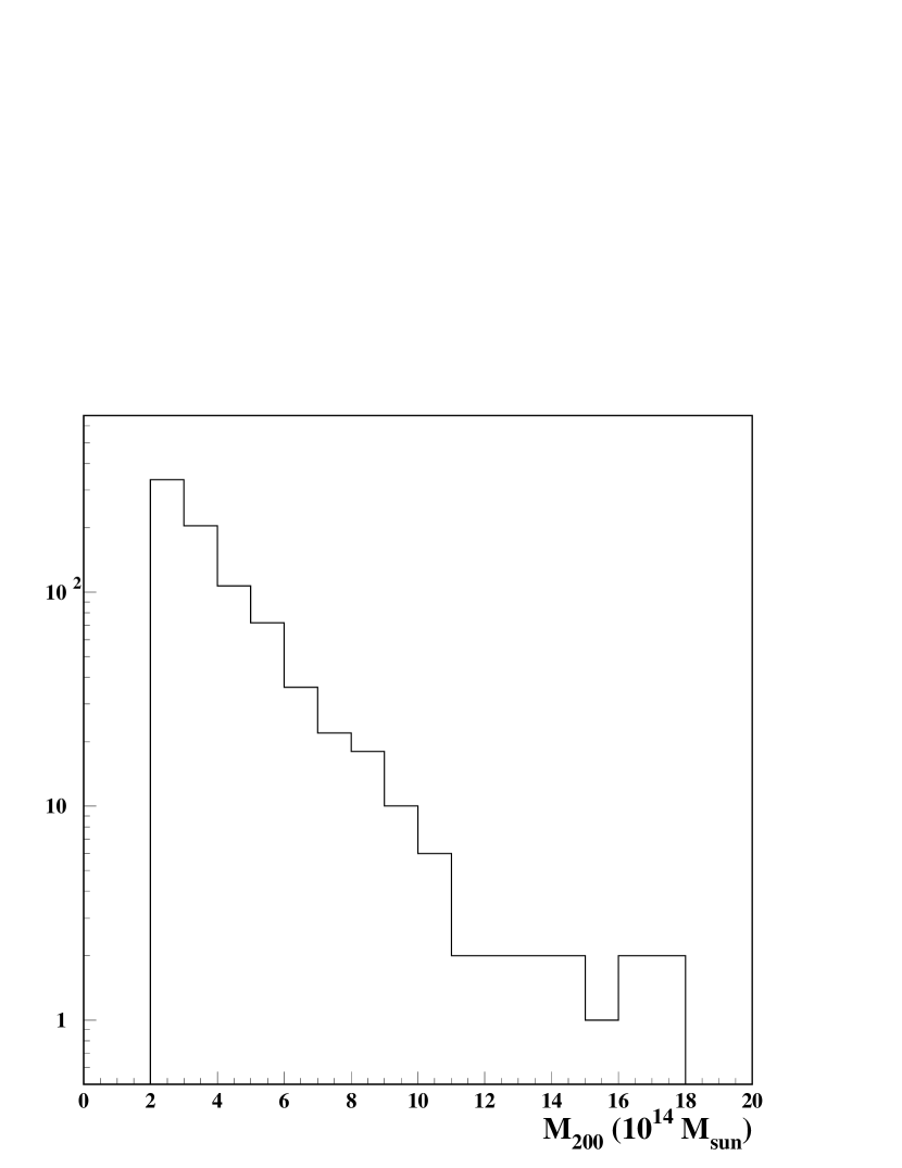
Figure 4: The mass distribution for our sample of inspected clusters. The masses were estimated from the $\sigma_{v}$-$N_{g}$ relation mentioned in the text and from Eqn. (1).

3 Search by Visual Inspection

Previous arc surveys have generally used visual inspection to locate arc candidates, which are then usually followed up with deeper imaging in better seeing.

The SDSS images of the 825 selected clusters were visually inspected for arcs. For each cluster, we used a SDSS coaddition code to build an image covering an angle corresponding to a physical scale of 1 Mpc (assuming $H_{0}=100$ km/s, $\Omega_{m}=0.3$, and $\Omega_{\Lambda}=0.7$). The inspector was then presented with 4 simultaneous images using the ds9 image display program: grayscale images of the $g$, $r$, and $i$ bands and a color image that combines the three bands. The grayscale images were displayed using the ds9 “zscale” algorithm, while the color image was displayed using a fixed surface brightness range (the same range was used for all clusters). A single author of this work (T.L.) scanned the 825 images, while three other authors inspected images of the 300 highest $N_{g}$ clusters in the sample. Candidates were recorded for later consideration and for potential follow-up observations (§5).

3.1 Visual Inspection Selection Function

A selection function is a prerequisite for the proper use of arc statistics to constrain cosmology. In order to calculate a selection function for our arc search, simulated arcs were added to a fraction of the images in our cluster sample. These objects were included before the images were inspected for arcs and without the knowledge of the scanner doing the visual inspection. Each added arc consisted of a section of a circle centered on the brightest cluster galaxy identified by the maxBCG algorithm. We added the arcs using uniform distributions in log peak surface brightness and in length-to-width ratio ($l/w=5-20$) in order to derive the arc detection efficiency as a function of these arc parameters. The simulated arcs have a flat spectrum in AB magnitudes, similar to typical observed gravitational arcs from other surveys (this makes the simulated arcs much bluer than the cluster galaxies). The typical length for the simulated arcs was $l\approx 10^{\prime\prime}$, and they were inserted in the images at $5^{\prime\prime}-45^{\prime\prime}$ from the brightest cluster galaxy (BCG). The simulated arcs have a surface brightness profile that is uniform along the tangential direction and is a gaussian along the radial direction, with a FWHM = $1.2^{\prime\prime}$ ($\approx w$), similar to the typical SDSS seeing. The selection functions obtained with this technique are presented in Figs. 5 and 6.

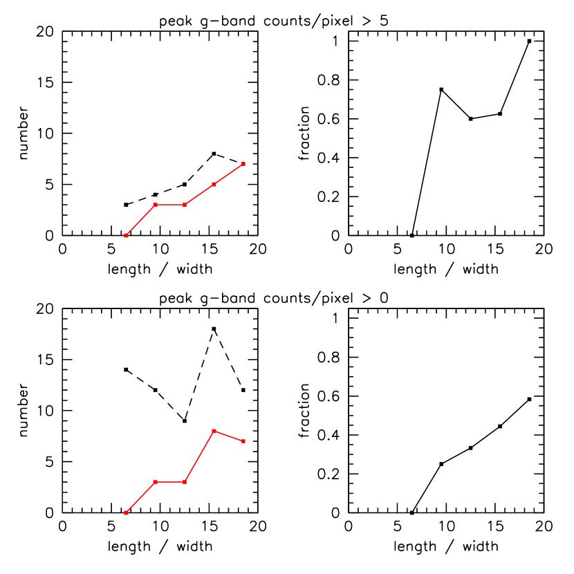
Figure 5: Efficency for finding simulated arcs as a function of the length-to-width ratio $l/w$. The panels on the left show the number of simulated arcs included in the images (dashed black) and the number of these arcs recovered by the visual inspection (solid red). The panels on the right show the efficiency for recovering the simulated arcs. The top panel shows the results for arcs with more than 5 counts/pixel in peak surface brightness (the conversion of counts per pixel to surface brightness is shown in Fig. 6) and the bottom panel shows the efficiency for the whole sample.

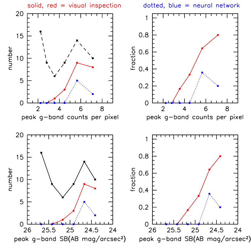
Figure 6: Efficiency for finding simulated arcs as a function of $g$-band peak surface brightness, in units of either counts per pixel (top panels) or AB magnitudes per arcsec² (bottom panels). The panels on the left show the number of simulated arcs included in the images (dashed black), the number recovered by the visual inspection (solid red), and the number recovered by the automated search (dotted blue). The panels on the right show the efficiency for recovering the simulated arcs.

For the visual inspection, the detection efficiency reaches 50% at about 24.8 mag/arcsec² in the peak g-band surface brightness and for $l/w\approx 10$. The primary causes for missed arcs are low surface brightness and small length-to-width ratio. However, the recovery efficiency does not reach 100% even for high $l/w$ ratio, high surface brightness arcs, due to blending problems with bright galaxies and stars on the images. Note that the measurement of our selection function is somewhat limited by small-number statistics, because we decided not to populate a significant fraction of our images with simulated arcs (we added 65 simulated arcs in total, i.e., to about 8% of the 825 inspected clusters).

4 Search by Algorithm

While sophisticated arc-finding algorithms have been published previously (e.g., Lenzen et al., 2004; Horesh et al., 2005; Alard, 2006; Starck et al., 2003; Seidel et al., 2006) we are not aware of an arc search that has been performed in a fully automated way. Clearly if we are to examine $10^{5}$ clusters we will need to use an algorithm (as opposed to a human eye inspection). We have developed such an algorithm, based on ideas taken from related techniques used in experimental particle physics for tracking particles in cloud and bubble chambers. In this work we will set a benchmark comparison between a simple algorithm for arc detection and a visual inspection.

4.1 The Algorithm

Our algorithm is composed of three steps: image preparation, candidate pre-selection, and final arc selection.

Step 1 is image preparation, where we scale the $g,r,i$ images by the variances of their respective sky backgrounds, normalize the variances to 1.0, average the three images together, and then run SExtractor (Bertin & Arnouts, 1996) to produce an object image. This step is intended to enhance the signal-to-background ratio of the arc-like objects. The averaging of the variance-normalized images follows the ideas of Szalay et al. (1999), and the intent is to produce an image where the pixel values are a $\chi^{2}$ of the hypothesis that the pixel consists of only sky. The SExtractor-produced object image has eliminated isolated pixels above threshold (due to noise) that do not belong to any object, retaining only pixels belonging to objects dectected above threshold. We perform a deblending of the SExtractor objects by separating each object into sub-objects which correspond to groups of contiguous pixels above threshold, and those sub-objects that are separated from another sub-object by fewer than 2 pixels are merged into one object.

Step 2 is candidate pre-selection, where the basic shape of the candidates is characterized by measuring the major and minor axes of each object, and where objects that show elongated shapes are kept for further study. The major axis ($r_{1}$) is defined as the largest distance between any pair of the $N$ pixels belonging to the object, and the minor axis ($r_{2}$) is defined as the maximum distance between pixels perpendicular to the main axis. Elongated objects, where $r_{1}/r_{2}\geq 1.4$, are chosen for further analysis. Step 2 simply reduces the number of objects to be studied, in order to reduce computation time per image. It is designed to be both complete and efficient, keeping $\approx 100\%$ of the arc-like objects while providing about a factor of 100 in rejection against the rest of the objects detected by SExtractor.

Step 3 is final arc selection, where the remaining objects have their radius of curvature measured. Those radii, plus other parameters measured in step 2, become the input for a neural net (NN) trained to select simulated arcs. The output of this NN is used to determine if an object is a good arc candidate. The radius of curvature ($R$) is measured using a least squares fit. The selection of good arc candidates then uses the following quantities:

• $r_{1}/(2\pi R)$: the fraction of the circumference covered by the arc. This is typically $>0.2$ for objects with significant curvature.

• $N/(\pi R^{2})$: the fraction of the circle area covered by pixels above threshold. This is typically $<0.15$ for good candidates.

• $\chi^{2}/N$: the goodness of fit.

• $r_{1}$: the length of the long axis. This ensures significant size for the candidates, $>20$ pixels (1 pixel $=0.396^{\prime\prime}$).

The 4 quantitites described above are then presented to a NN with 8 nodes in a hidden layer and the output is trained (by back propagation) to identify simulated arcs. The NN was trained using a separate sample of 100 bright simulated arcs, where the peak surface brightness was fixed at 20 counts per pixel in the $g$ band.

4.2 Algorithm Selection Function

The efficiency obtained with this algorithm is somewhat lower than that seen for the human scan and is shown in Fig. 6. The detection efficiency reaches 40% at 24.7 mag/arcsec² in the $g$ band and for $l/w\approx 10$; the curve is consistent with the eye scan curve shifted to a brighter surface brightness by $\approx 0.4$ mags. More development will be needed to bring this algorithm to the level of efficiency of the visual inspection. However, this analysis provides a quantitative benchmark for the comparison of a human search with a simple algorithm search applied to the same cluster sample.

5 Candidate Follow-up

The six best candidates, all from the visual inspection, were selected for follow-up. These arc candidates were observed using the SPIcam imager on the Apache Point Observatory 3.5-meter telescope. Images were takin in the SDSS $g$, $r$, and $i$ filters. The observations were done the night of April 29-30, 2006, during dark time. Table 1 shows the amount of time spent observing each object with the three filters. The images were reduced using standard bias subtraction and flat-fielding techniques. The images were also registered and coadded. Typical seeing on the individual images ranged from $1.1^{\prime\prime}$ to $1.5^{\prime\prime}$.

The candidates were inspected by the authors and discarded based on judgements that they were most likely “junk” or edge-on galaxies. Room for improvement in this system exists and we plan on putting into place a set of criteria for systematic follow-up. The criteria useful for SDSS data are obvious from an examination of Fig. 1: $l/w$, surface brightness, radius of curvature, and color.

Table 1: Candidate Observations

Name	RA	Dec	z	g (min)	r (min)	i (min)
SDSS+139.5+51.7+0.24	09:17.59.5	51:42:06	0.24	15	5	5
SDSS+184.4+3.6+0.08	12:17:28.0	03:36:17	0.08	15	5	5
SDSS+117.7+17.7+0.19	07:50:48.9	17:40:43	0.19	15	5	5
SDSS+175.3+5.8+0.12	11:41:13.5	05:48:28	0.12	15	5	5
SDSS+205.5+26.4+0.10	13:41:49.1	26:22:25	0.10	15	5	5
SDSS+139.1+5.9+0.14	09:16:21.3	05:53:18	0.14	15	5	5

Note. — SPIcam observations. Exposure times are given in minutes. The redshifts quoted for the clusters are photometric redshifts from the maxBCG algorithm and have a dispersion of $\sigma_{z}=0.015$.

6 Results of the Searches

Our survey of 825 SDSS galaxy clusters resulted in no convincing candidates for giant gravitational arcs.

The selection function we have computed shows that we are $\geq 50\%$ efficient at SB $\leq 24.8$ mags/arcsec² and for $l/w\geq 10$. The latter, given our mean seeing of $1.4^{\prime\prime}$, corresponds to arcs longer than $14^{\prime\prime}$. Fig. 7 shows the surface brightness distribution of the arcs found by Lynds & Petrosian (1989, in seeing of $\sim 1.0$”), by Luppino et al. (1999, $\sim 0.90^{\prime\prime}$, their Table 2), by Zaritsky & Gonzalez (2003, $\sim 0.55^{\prime\prime}$), and by Gladders et al. (2003, $\sim 0.85^{\prime\prime}$). These are all the published ground based surveys, and no attempt to homogenize the seeing has been made. The surface brightnesses have been converted into the AB system from the Vega system. We assume that the arcs have flat spectra so that no change is necessary for the different bandpasses. We see from Figure 7 that our surface brightness limit is in fact exceeded by the majority of these arcs. The observed surface brightness for arcs that are unresolved in width is a function of the seeing obtained, and the data here include a variety of seeing. However, all are better than our sample’s mean seeing of $1.4^{\prime\prime}$, so if this plot were homogenized to the SDSS seeing most of these arcs would fall below our surface brightness limit. Seeing is thus the dominant limiting factor in our efficiency, and it is the relatively large PSF of the SDSS data that limits our detection to high surface brightness, quite long arcs with $l/w\geq 10$. On the other hand, the arcs that we can in fact find in the SDSS will therefore also be particularly interesting objects for follow-up observations.

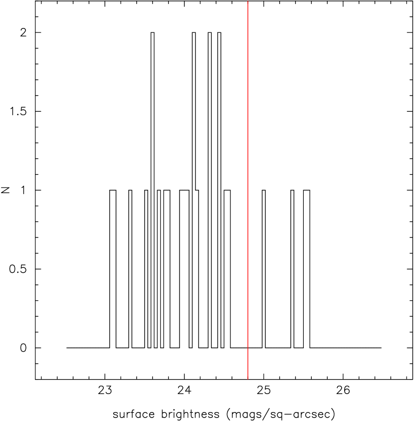
Figure 7: The surface brightnesses of the arcs found in previous ground based searches. The surface brightness is reported in the AB system; given the simplifying assumption of a flat spectrum arc, we need not report the bandpass, though the data were in fact observed through a variety of filters ($B,V,R,I$). The vertical red line is the $50\%$ efficiency limit of our visual search selection function.

6.1 Upper Limits on the Observable Arc Production

We use our search results to establish upper limits on the production of observable giant arcs by galaxy clusters. Assuming Poisson statistics, an observation of 0 arcs for a given inspected cluster indicates that the 95% C.L. upper limit on the expected number of observable arcs per cluster is 3 (i.e., the probability of observing 0 events for a Poisson distribution with mean 3 is $3^{0}e^{-3}/0!\approx 0.05=1-0.95)$. Then, given a null result after inspecting $N_{i}$ clusters in a redshift bin $i$, the 95% C.L. upper limit on the expected number of observable arcs per cluster, $\Sigma^{(i)}_{95\%}$, may be determined from the product of the individual Poisson probabilities using the relation

$$[\ (\Sigma^{(i)}_{95\%})^{0}\ e^{-\Sigma^{(i)}_{95\%}}\ /\ 0!\ ]^{N_{i}}=e^{-\Sigma^{(i)}_{95\%}N_{i}}=0.05\ ,$$ (2)

from which we find that

$$\Sigma^{(i)}_{95\%}=\frac{3}{N_{i}}.$$ (3)

$\Sigma^{(i)}_{95\%}$ is shown in Fig. 8 for clusters with estimated masses $M_{200}>2\times 10^{14}M_{\sun}$ and $M_{200}>4\times 10^{14}M_{\sun}$. It should be noted that our upper limits correspond to arcs observable by the SDSS according to the efficiency for detection shown in Figs. 5 and 6. The lower panel in Fig. 8 corresponds to the more massive clusters ($M_{200}>4\times 10^{14}M_{\sun}$) in our sample, and from the plot it is clear that we only have the statistics for a significant limit in the range $0.1<z<0.3$.

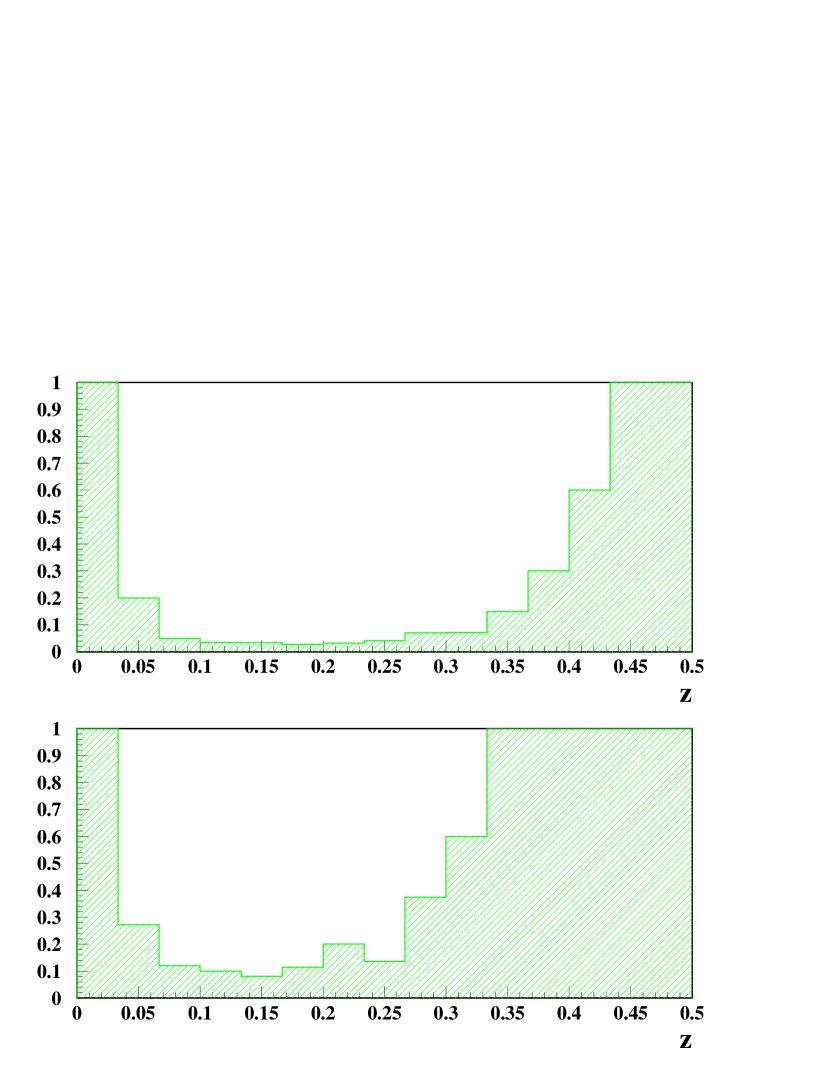
Figure 8: The 95% C.L. upper limit for the probability for a cluster to produce a gravitational arc visible in SDSS imaging, assuming Poisson statistics in our sample of 825 clusters. The limit is shown as a function of redshift for $M_{200}=2-4\times 10^{14}M_{\sun}$ clusters in the top panel and for $M_{200}>4\times 10^{14}M_{\sun}$ clusters in the bottom panel.

6.2 Comparison With Previous Works

In order to understand the compatibility of our results with previous arc searches, we perform a direct comparison with these searches over similar redshifts. The cluster selection function is a considerable source of uncertainty which is hard to quantify for this comparison, ans so to reduce the impact of this effect we have selected on each sample clusters with similar mass estimators. The sample of X-ray luminous galaxy clusters constructed by Smith et al. (2005) is a good place to start. This sample has a total of 10 rich clusters with $M_{200}>4\times 10^{14}M_{\sun}$ at $0.17\leq z\leq 0.26$, where the mass is estimated from X-ray luminosities (Allen et al., 2003). The sample was imaged with HST and the geometrical properties of the arcs were published by Sand et al. (2005). In order to estimate the expected number of arcs observable in the SDSS, the parameters of the arcs are degraded from those observed in HST imaging (with a typical PSF of 0.15”) to the image quality of the SDSS (with a typical PSF of 1.4”). This conversion is done assuming that the arc is well resolved in HST imaging, i.e., that the width is entirely due to the object, not the PSF. The width is then increased by adding in quadrature the average seeing for the SDSS, effectively reducing the $l/w$ ratio. The increased width results in an increased area for the object, which translates into a reduction in surface brightness. Of the arc candidates observed with HST in these clusters, only 3 remain with $l/w>10$ after degradation to SDSS seeing. Of the surviving arcs only 1 has a surface brightness inside our detection limit. Thus the sample of Smith et al. (2005) gives a 10% probability of having an arc observable by SDSS for clusters with $M_{200}>4\times 10^{14}M_{\sun}$ and $0.15<z<0.3$. This result lies inside the 95% C.L. presented in Fig. 8.

A similar comparison can be done with the Luppino et al. (1999) sample of 38 EMSS X-ray selected clusters with $L_{x}\geq 2\times 10^{44}$ ergs/sec at $0.15\leq z\leq 0.82$. As before, the parameters for the arcs were transformed into expected parameters for the SDSS using the seeing applicable to each arc observation carried out by Luppino et al. (1999). After this procedure, no arc from this sample is expected to be observable in SDSS imaging. Again, this result is consistent with the upper limits derived from our analysis.

The results obtained in this work are also consistent with a search for giant gravitational arcs in the RCS (Gladders et al., 2003). The RCS cluster sample covers a redshift range $0.35<z<0.95$, and after visual inspection of approximately 900 clusters with $M_{200}>4\times 10^{14}M_{\sun}$, 3 strong lensing systems with giant arcs were found, all of them with $z>0.60$. The result from the RCS indicates a smaller probability for a low redshift cluster to produce an arc, compared with a cluster of similar mass at higher redshifts. The bulk of the clusters used for the arc search in the present work have redshifts $0.1<z<0.3$, lower than the arc clusters found by the RCS, and so our null result is also consistent with the RCS result that low-redshift clusters are less efficient for the production of arcs.

We are aware of 4 giant arc systems recovered or discovered in single-pass SDSS imaging: one found by the RCS (Gladders et al., 2003, see below), one found by Sand et al. (2004, RX J1133), a new system described in the Appendix, and another new system that is described in Allam et al. (2006). Three of the arc systems are lensed by clusters with $N_{g}\sim 10-20$, beneath the threshold of our current work, and these also have $0.35\leq z\leq 0.45$, beyond our catalog redshift limit though well within the reach of SDSS cluster finders. The fourth is RCS1419.2+5326 at $z=0.64$: our cluster finders can discover objects with these properties, but with $N_{g}\sim 5$ (as observed by the SDSS; the real $N_{g}$ is much higher) the catalogs are far from the $90\%$ efficiency level of the $z<0.3$ catalogs (the actual efficiency may be of order $1-5\%$). It is worth noting that the two high surface brightness arcs found by Lynds & Petrosian (1989) are just south of the limits of the SDSS Stripe 82 region. Had both clusters been 1 degree farther north, they would likely have been found in our survey.

7 Summary

The potential for observing arcs in SDSS imaging has been demonstrated by the observation of known arc systems in the multiband imaging of the survey (see Fig. 1) and by the discovery of new arcs (this paper and Allam et al., 2006). In this work, we presented a systematic search for gravitational arcs in a sample of SDSS clusters. A total 825 clusters with $N_{g}>20$ (corresponding to $M\gtrsim 2\times 10^{14}M_{\sun}$) have been visually inspected for arcs and have also been processed with an automated arc search algorithm. The efficiency of arc detection for both techniques has been quantified by using simulated arcs added to the inspected images. The results indicate a significantly higher efficiency for the eye scan and point to the need for developing a more efficient algorithm for the automated search. No gravitational arcs were seen in the sample of clusters analyzed. This result is consistent with previous surveys done over a similar redshift range ($0.1<z<0.3$).

8 Acknowledgements

Funding for the SDSS and SDSS-II has been provided by the Alfred P. Sloan Foundation, the Participating Institutions, the National Science Foundation, the U.S. Department of Energy, the National Aeronautics and Space Administration, the Japanese Monbukagakusho, the Max Planck Society, and the Higher Education Funding Council for England. The SDSS Web Site is http://www.sdss.org/.

The SDSS is managed by the Astrophysical Research Consortium for the Participating Institutions. The Participating Institutions are the American Museum of Natural History, Astrophysical Institute Potsdam, University of Basel, Cambridge University, Case Western Reserve University, University of Chicago, Drexel University, Fermilab, the Institute for Advanced Study, the Japan Participation Group, Johns Hopkins University, the Joint Institute for Nuclear Astrophysics, the Kavli Institute for Particle Astrophysics and Cosmology, the Korean Scientist Group, the Chinese Academy of Sciences (LAMOST), Los Alamos National Laboratory, the Max-Planck-Institute for Astronomy (MPIA), the Max-Planck-Institute for Astrophysics (MPA), New Mexico State University, Ohio State University, University of Pittsburgh, University of Portsmouth, Princeton University, the United States Naval Observatory, and the University of Washington.

Appendix A Appendix: Hall’s Arc

We report here an arc discovered serendiptously by one of us (P.B.H) in 2004. It is widely known inside the SDSS Collaboration but has not been published previously. The purely serendipitous discovery was made during inspection of the images of spectra classified UNKNOWN (the initial reduction of the SDSS spectrum had bad spectrophotometry and could not be classified). There is a cluster clearly visible in the images: the BCG has a SDSS spectrum and is at $z=0.44$, and it is coincident with NVSS J014656-092952. The SDSS spectrum shows two objects superimposed, the $z=0.44$ galaxy and a star – the latter is what the SDSS pipeline reports.

We ran the maxBCG code at the position of the BCG and measured $N_{g}=12$, but this is a lower limit. The cluster is above the redshift where the $N_{g}$ is complete – at this redshift two effects compromise the $N_{g}$ measurement: (1) $0.4L^{\star}$ is fainter than the useful limiting magnitude of the SDSS, and (2) the colors of objects near $0.4L^{\star}$ become noisy enough to scatter outside the color box used to determine cluster membership. A correction must be applied to $N_{g}$ for these effects. As we are not attempting to use this arc in our analysis we defer the measurement of the corrected $N_{g}$ to a later paper. We have tabulated our information about the cluster in Table 2.

There are three arcs. The longest one was split by the SDSS photometry pipeline Photo into two objects, a and b. We report on the object parameters in Table 3. Three of the four objects have photometric redshifts of about 0.6-0.7; the fourth is about $3\sigma$ away (though we note that for faint objects $r>20$ the SDSS photometric redshifts are less reliable because the spectroscopic training sets available are less extensive than at brighter magnitudes). We measured the parameters of the three arcs in the SDSS $g$-band image. These are listed in Table 4. It is likely that we would have found this arc in our survey (if it had been in our sample catalog) because it is remarkably clean: there are no stars or cluster galaxies that are projected onto the images of the arcs. Deeper imaging data for this system may be found in Hennawi et al. (2006).

Table 2: Hall’s Arc: the Cluster

Name	RA	Dec	$z$	$N_{g}$
SDSS+26.733-9.497+0.44	01:46:56.00	-09:29:52.4	0.44	$\geq 12$

Table 3: Hall’s Arc: Positions, Magnitudes, and Photo-z’s

Arc	RA	Dec	$g$	$u-g$	$g-r$	$r-i$	$i-z$	$z_{phot}$
1a	26.73210	-9.50009	$21.85\pm 0.15$	$1.3\pm 1.4$	$0.57\pm 0.21$	$0.68\pm 0.19$	$0.09\pm 0.51$	$0.61\pm 0.14$
1b	26.73051	-9.49967	$21.81\pm 0.21$	$0.39\pm 0.92$	$0.75\pm 0.27$	$0.63\pm 0.22$	$-1.8\pm 2.6$	$0.57\pm 0.23$
2	26.73063	-9.49525	$21.66\pm 0.10$	$0.45\pm 0.46$	$0.53\pm 0.14$	$0.73\pm 0.12$	$0.29\pm 0.28$	$0.67\pm 0.08$
3	26.73641	-9.49673	$21.77\pm 0.15$	$0.66\pm 0.81$	$0.03\pm 0.27$	$0.15\pm 0.39$	$-1.1\pm 2.1$	$0.15\pm 0.15$

Note. — SDSS data. We retain the SDSS decimal degrees convention for RA and Dec. The magnitudes and colors are SDSS model magnitudes and are corrected for extinction (see Adelman-McCarthy et al., 2006, and references therein).

Table 4: Hall’s Arc: Arc Parameters

Arc	$l$	$l/w$	mean SB (mag/arcsec2)
1	$17.2^{\prime\prime}$	11.2	24.5
2	$10.0^{\prime\prime}$	6.5	24.6
3	$3.8^{\prime\prime}$	2.5	23.7

Note. — SDSS $g$-band measurements. The $g$-band PSF is $1.53^{\prime\prime}$.

Table 5: List of the most 20 most massive inspected clusters in our sample. The full sample is available electronically.

Name	RA	DEC	$z$	$N_{g}$	$M_{200}$
SDSS+239.6+27.2+0.11	239.634	27.1808	0.109	94	31.2
SDSS+230.6+27.7+0.08	230.6	27.7144	0.083	88	28.1
SDSS+213.6-00.3+0.13	213.618	-0.3301	0.133	69	17.7
SDSS+117.7+17.7+0.19	117.721	17.6768	0.192	68	16.7
SDSS+258.2+64.0+0.08	258.227	63.9924	0.081	67	17.2
SDSS+227.8+05.8+0.08	227.75	5.7828	0.081	65	16.3
SDSS+197.9-01.3+0.20	197.886	-1.3329	0.203	65	15.3
SDSS+234.9+34.4+0.25	234.893	34.4369	0.249	63	14.1
SDSS+250.1+46.7+0.25	250.098	46.7028	0.242	62	13.7
SDSS+110.4+36.7+0.15	110.36	36.7383	0.148	62	14.4
SDSS+227.6+33.5+0.12	227.584	33.486	0.116	59	13.4
SDSS+250.8+13.4+0.20	250.843	13.363	0.199	58	12.5
SDSS+126.3+47.1+0.13	126.32	47.1424	0.129	58	12.9
SDSS+203.8+41.0+0.26	203.818	41.0132	0.264	55	10.9
SDSS+139.5+51.7+0.24	139.481	51.7163	0.236	54	10.7
SDSS+255.7+34.1+0.11	255.69	34.0611	0.109	54	11.5
SDSS+228.8+04.4+0.11	228.823	4.397	0.107	53	11.1
SDSS+137.3+11.0+0.18	137.329	10.9857	0.179	53	10.7
SDSS+184.4+03.6+0.08	184.381	3.6157	0.089	52	10.9
SDSS+216.5+37.8+0.16	216.475	37.7915	0.164	50	9.7

References

- Adelman-McCarthy et al. (2006) Adelman-McCarthy, J.K., et al. 2006, ApJS, submitted
- Allam et al. (2006) Allam, S. S., Tucker, D. L., Lin, H., Diehl, H. T., Annis, J., Buckley-Geer, & Frieman, J.A., ApJL, submitted, astro-ph/0611138.
- Alard (2006) Alard, C. 2006, A&A, submitted, astro-ph/0606757.
- Allen et al. (2003) Allen, S. W., Schmidt, R. W., Fabian, A. C., & Ebeling, H. 2003, MNRAS, 342, 287
- Bahcall et al. (2003) Bahcall, N. A. et al. 2003, ApJS, 148, 243
- Bartelmann et al. (1998) Bartelmann, M., Huss, A., Colberg, J. M., Jenkins, A., & Pearce, F. R. 1998, A&A, 330, 1
- Bertin & Arnouts (1996) Bertin, E., & Arnouts, S. 1996, A&AS, 117, 393
- Bolton et al. (2006) Bolton, A. S., Burles, S., Koopmans, L. V. E., Treu, T., & Moustakas, L. A. 2006, ApJ, 638, 703
- Borgani et al. (2004) Borgani, S., et al. 2004, MNRAS, 348, 1078
- Bryan & Norman (1998) Bryan, G.L., & Norman, M.L. 1998, ApJ, 495, 80
- Campusano et al. (2006) Campusano, L. E., Cypriano, E. S., Sodré, L., Jr., & Kneib, J.-P. 2006, EAS Publications Series, 20, 269
- Couch & Ellis (1995) Couch, W., & Ellis, R. 1995, Science, 268, 199
- Cypriano (2002) Cypriano, E. S. 2002, Ph.D. thesis, Universidade de São Paulo.
- Dalal et al. (2004) Dalal, N., Holder, G., & Hennawi, J. F. 2004, ApJ, 609, 50
- Eke et al. (1998) Eke, V., Navarro, J., & Frenk, C. 1998, ApJ, 503, 569.
- Evrard et al. (2002) Evrard, A. E., et al. 2002, ApJ, 573, 7
- Frenk et al. (1999) Frenk, C. S., et al. 1999, ApJ, 525, 554
- Fukugita et al. (1996) Fukugita, M., Ichikawa, T., Gunn, J.E., Doi, M., Shimasaku, K., & Schneider, D.P. 1996, AJ, 111, 1748
- Gladders et al. (2003) Gladders, M. D., Hoekstra, H., Yee, H. K. C., Hall, P. B., & Barrientos, L. F. 2003, ApJ, 593, 48
- Grossman & Narayan (1988) Grossman, S. A., & Narayan, R. 1988, ApJ, 324, L37
- Gunn et al. (1998) Gunn, J.E., et al. 1998, AJ, 116, 3040
- Gunn et al. (2006) Gunn, J.E., et al. 2006, AJ, 131, 2332
- Mohr et al. (2001) Haiman, Z., Mohr, J. J., & Holder, G. P. 2001, ApJ, 553, 545
- Hansen et al. (2005) Hansen, S. M., McKay, T. A., Wechsler, R. H., Annis, J., Sheldon, E. S., & Kimball, A. 2005, ApJ, 633, 122
- Heitman et al. (2005) Heitmann, K., Ricker, P. M., Warren, M. S., & Salman, H. 2005, ApJS, 160, 28
- Hennawi et al. (2005) Hennawi, J. F., Dalal, N., Bode, P., & Ostriker, J.P. 2005, ApJ, submitted, astro-ph/0506171
- Hennawi et al. (2006) Hennawi, J.F., et al. 2006, ApJ, submitted, astro-ph/0610061
- Ho & White (2005) Ho, S., & White, M. 2005, Astroparticle Physics, 24, 257
- Hogg et al. (2001) Hogg, D.W., Finkbeiner, D.P., Schlegel, D.J., & Gunn, J.E. 2001, AJ, 122, 2129
- Horesh et al. (2005) Horesh, A., Ofek, E. O., Maoz, D., Bartelmann, M., Meneghetti, M., & Rix, H.-W. 2005, ApJ, 633, 768
- Ivezic et al. (2004) Ivezic, Z., et al. 2004, AN, 325, 583
- Johnston et al. (2006) Johnston, D.E., Sheldon, E.S., Tasitsiomi, A., Frieman, J.A., Wechsler, R., & McKay, T.A. 2006, ApJ, submitted, astro-ph/0507467
- Kneib et al. (1996) Kneib, J.-P., Ellis, R. S., Smail, I., Couch, W.J., & Sharples, R. M. 1996, ApJ, 471, 643
- Koester et al. (2006a) Koester, B., et al. 2006a, in preparation
- Koester et al (2006b) Koester, B., et al. 2006b, ApJ, submitted
- Lenzen et al. (2004) Lenzen, F., Schindler, S., & Scherzer, O. 2004, A&A, 416, 391
- Li et al. (2005) Li, G.-L., Mao, S., Jing, Y. P., Bartelmann, M., Kang, X., & Meneghetti, M. 2005, ApJ, 635, 795L
- Luppino et al. (1999) Luppino, G. A., Gioia, I. M., Hammer, F., Le Fèvre, O., & Annis, J. A. 1999, A&AS, 136, 117
- Lupton et al. (2001) Lupton, R. H., Gunn, J. E., Ivezić, Z., Knapp, G. R., Kent, S., & Yasuda, N. 2001, in ASP Conf. Ser. 238, Astronomical Data Analysis Software and Systems X, ed. F.R. Harnden, Jr., F.A. Primini, & H.E. Payne (San Francisco: Astr. Soc. Pac.), p. 269
- Lynds & Petrosian (1989) Lynds, R., & Petrosian, V. 1989, ApJ, 336, 1
- Miralda-Escudé (1993) Miralda-Escudé, J. 1993, ApJ, 403, 497
- Oguri et al. (2003) Oguri, M., Lee, J., & Suto, Y. 2003, ApJ, 599, 7
- Oguri et al. (2006) Oguri, M. et al. 2006, AJ, 132, 999
- Pier et al. (2003) Pier, J.R., Munn, J.A., Hindsley, R.B., Hennessy, G.S., Kent, S.M., Lupton, R.H., & Ivezic, Z. 2003, AJ, 125, 1559
- Pindor et al. (2003) Pindor, B., Turner, E. L., Lupton, R. H., & Brinkmann, J. 2003, AJ, 125, 2325
- Press & Schechter (1974) Press, W. H., & Schechter, P. 1974, ApJ, 187, 425
- Sand et al. (2004) Sand, D.J., et al. 2004, ApJ, 604, 88
- Sand et al. (2005) Sand, D. J., Treu, T., Ellis, R. S., & Smith, G. P. 2005, ApJ, 627, 32
- Seidel et al. (2006) G. Seidel, M. Bartelmenn, astro-ph/0607547 (2006).
- Sheldon et al. (2001) Sheldon, E.S., et al., 2001, ApJ, 554, 881
- Sheldon (2006) Sheldon, E.S., et al. 2006, ApJ, submitted
- Smail et al. (1996) Smail, I., Dressler, A., Kneib, J.-P., Ellis, R.S., Couch, W. J., Sharples, R. M., & Oemler, A. 1996, ApJ, 469, 508
- Smith et al. (2005) Smith, G. P., Kneib, J.-P., Smail, I., Mazzotta, P., Ebeling, H., & Czoske, O. 2005, MNRAS, 359, 417
- Smith et al. (2002) Smith, J.A., et al. 2002, AJ, 123, 2121
- Starck et al. (2003) Starck, J.,L., Donoho, D.,L., & Candes, E.,J., 2003, A&A, 398,785
- Stoughton et al. (2002) Stoughton, C., et al. 2002, AJ, 123, 485
- Soucail et al. (1987) Soucail, G., Fort, B., Mellier, Y., & Picat, J. P. 1987, A&A, 172, L14
- Szalay et al. (1999) Szalay, A. S., Connolly, A. J., & Szokoly, G. P. 1999, AJ, 117, 68
- Tucker et al. (2006) Tucker, D., et al. 2006, AN, 327, 821
- Voit (2005) Voit, G. M. 2005, Rev. Mod. Phys., 77, 207
- Wambsganss et al. (2004) Wambsganss, J., Bode, P., & Ostriker, J. P. 2004, ApJ, 606, L93
- Wu & Hammer (1993) Wu, X.-P., & Hammer, F. 1993, ApJ, 463, 404
- York et al. (2000) York, D. G. et al. 2000, AJ, 120, 1579
- Zaritsky & Gonzalez (2003) Zaritsky, D., & Gonzalez, A. H. 2003, ApJ, 584, 691