The study of colliding molecular clumps evolution

Abstract

The results of study of the gravitational fragmentation in the interstellar medium (ISM) by clump-clump collisions are presented. We suggest, that collision of clumps, that are subparts of Giant Molecular Clouds (GMC) may be on of the basic mechanism, which result to ISM fragmentation and define the dynamical as well as statistical characteristics (e.g. the mass spectra) of protostellar condensation.

In the present paper, we describe our $3D$ SPH-modeling, in isothermal approximation, of supersonic collisions of two identical clumps with a few variants of initial impact parameters ($\beta$), that cover the wide range.

Our results shown, that at all $\beta$ in system began intensive fragmentation. The resulting fragments mass function depend from initial impact parameter. The obtained mass spectra have the slopes in a good enough agreement with observational data for our Galaxy – especially for large impact parameters, which are more realistic as for large clumps ensembles.

KEY WORDS     ISM, fragmentation, molecular clouds collisions, clumps mass spectra, SPH method

1 Introduction

Nearly the half mass of gas in our Galaxy are concentrated in giants molecular clouds (GMC) with typical sizes in tens parsecs, masses $10^{5}-10^{6}\,\mathfrak{M}_{\odot}$ and temperatures $T\lesssim 20\textrm{K}$ [1, 2, 3]. The mean number density in GMC is equal to $10^{2}-10^{3}\;\textrm{cm${}^{-3}$}$, but in some regions it can reaches up to $10^{6}\;\textrm{cm${}^{-3}$}$ [2]. There are about 4000 such objects in Galaxy and this objects mainly concentrate in the Galaxy disc [1, 2, 3].

The GMC tightly connect with some other objects in our Galaxy – such as IR-sources, masers, compact H II zones, T Tau stars, Herbig-Haro objects, O-association etc. This connection show the clear evidence of star formation process in GMC at present.

The hight resolution radio observations of GMC in molecular lines, show their clear fragmentary structure on all hierarchy levels down to parsec’s fractions. In first approximation we can describe the GMCs as a complex of smaller and denser condensations (clumps), embedded into tenuous gas medium.

The typical clump have a mass in $10^{3}-10^{4}\;\,\mathfrak{M}_{\odot}$ and size in a few parsecs. It content yet more small and dense cores with masses in several solar mass and sizes in parsec’s fraction [2]. As a good examples of such clouds complexes we can brought the $\rho$ Oph [4], M17 SW [5] and Tauri molecular clouds complex [6].

The numerous observational data about molecular clouds indicate the complex gas flows and clumps chaotic motions inside GMC. There are strong turbulence inside clumps, but tenuous gas ”background” have a more regular kinematics. The dependence of velocity dispersion $\sigma$ from size of consider region can be approximated by the power law $\sigma\propto L^{0.38}$ [7]. Here $\sigma$ is total 3D-rms velocity deviation for all internal motions including large-, small-scale and thermal gas motions (for H₂ clumps at temperature in a few tens of Kelvins the mean quadratic velocity of thermal motions is negligible by comparison with two first components). $\sigma$ is about $1\;\textrm{km/s}$ for $R\approx 2\;\textrm{pc}$ or $\mathfrak{M}\approx 2000\;\,\mathfrak{M}_{\odot}$.

This discovered dependence is very similar to Kolmogorov law for distribution of velocity dispersion at subsonic turbulence ($\sigma\propto L^{0.33}$) and it is possibly, that all seen us interstellar movements is parts of a single hierarchy of interstellar turbulence.

At that time the rms velocity dispersion of molecular clouds and clumps itself have mainly flat spectrum in wide mass range (up to four orders) with average value around $5-10\;\textrm{km/s}$ [8, 9].

Usually, the GMC, having masses $10^{5}\!-\!10^{6}\,\mathfrak{M}_{\odot}$, may contain a tens of clumps with typical masses by order $10^{3}\!-\!10^{4}\,\mathfrak{M}_{\odot}$ [10]. Of course, chaotically moving at supersonic velocities, they can collide each with other. Many authors consider this mechanism as one of the possible source of ISM fragmentation and formation of initial mass function (MF) of protostellar condensations.

It is interesting to note, that as GMC, as clumps and cores inside its have almost the same mass spectra in mass range from $10^{-4}$ to $10^{4}\;\,\mathfrak{M}_{\odot}$ [11]. This may point to common mechanism of their formation. For example, just such result was obtained in special N-body modeling of collisional buildup of molecular clouds [12], that gave observational mass- and velocity spectra for obtained objects.

So, interclouds collisions have a great interest for its study, including a numerical simulations. First, two-clouds isothermal collisions are studied: for identical rotating clouds [13], non-rotating clouds with different masses [14] and collisions of identical clouds with taken into account cooling/heating processes [15, 16].

Simulations with using great particle numbers ($\sim\!10^{5}-10^{6}$) and, therefore, with hight resolution require sufficient CPU consumptions even for supercomputers. In consequence of that, they carrying out either without integrating of energy equation, but with barotropic state equation $p=p(\rho)$ [17], or simply in isothermal approximation [18].

In Monaghan & Varnas [15] and Bhattal et al. [17] the system of 48 and 1000 clouds correspondingly was considered. But even in such rich complexes the main role play just a pair collisions [18].

The most of such works were carried out without quantitative analysis of fragmentation. Thus, only in Bhattal et al. [17] and Gittins et al. [18] the masses of fragments are evaluated. Additionally, in the last work qualitative analysis of IMF is given for which the fragments are defined as a single sink particles without any internal structure, etc [see 19, for more details].

In our work we carried out simulation of isothermal supersonic collisions of two identical molecular clumps with aim of more detailed fragmentation study and mass distribution analysis of obtained fragments. For fragments finding we apply the modified variant of well-known ”friends-of-friends” algorithm (FOF).

2 The Method

2.1 Hydrodynamics

For gas process modeling we use the Smoothed Particle Hydrodynamics method (SPH), which was independently suggested by Lucy [20] and Gingold & Monaghan [21].

As in the well-known N-body algorithm, modeling system in SPH is represented by a set of computational particles which characterized by mass, position, linear and angular momentums and energy. Besides, each particle is diffusive one and additionally have some hydro- and thermodynamical parameters (such as density and thermal energy), defined for its ”center” by interpolating from nearest neighborhood. Partially overlapping, SPH-particles gives the average weighing contributes to local properties of medium, according with their internal distribution profile.

So, the smoothing estimate of any physical parameter $f({\bf r})$ in SPH is:

$$\langle f({\bf r})\rangle=\int f({\bf r}^{\prime})W({\bf r}-{\bf r}^{\prime},h)\;d{\bf r}^{\prime}\approx\sum_{j=1}^{N}m_{j}\frac{f({\bf r}_{j})}{\rho_{j}}W({\bf r}_{i}-{\bf r}_{j},h_{i}),$$ (1)

where the integral is taken over entire space and summation is over all $N$ particles, $h$– so-called smoothing length, $W({\bf r}-{\bf r}^{\prime},h)$ – interpolating smoothing kernel, which must satisfy to two simple conditions: $\int W({\bf r}-{\bf r}^{\prime},h)\;d{\bf r}^{\prime}\equiv 1\;\textrm{and}\;\lim_{h\to 0}W({\bf r}-{\bf r}^{\prime},h)\!=\!\delta({\bf r}-{\bf r}^{\prime}).$

Yet another SPH features is that it need not in finite-differences for gradients calculating. Instead of this we must only differentiate the smoothing kernel and then smooth interesting parameter as in (1):

$$\langle\nabla f({\bf r})\rangle=\int f({\bf r}^{\prime})\nabla W({\bf r}-{\bf r}^{\prime},h)\;d{\bf r}^{\prime}\approx\sum_{j=1}^{N}m_{j}\frac{f({\bf r}_{j})}{\rho_{j}}\nabla W({\bf r}_{i}-{\bf r}_{j},h_{i}).$$ (2)

The concrete form of kernel is chosen from reason, that non-zero contribution to local hydrodynamical properties must take only the nearest particles. Smoothing length $h$ define a scale of smoothing and so the spatial resolution.

The great flexibility of SPH is provided by absence of any restriction neither on system geometry, nor on admissible range of varying of dynamics parameters, easiness of kernel change (that is equal to change of finite-difference scheme in grid methods), variety of equation symmetrization means, artificial viscosity forms, etc.

Being hydrodynamics extension of earlier N-body method, SPH can naturally include it, as a one of its parts, for modeling collisionless components (as a dark matter). For handle with selfgravity field SPH use either grid methods to solve of Poisson’s equation, or TREE-algorithm [22], or, at last, direct summation of all particle-particle interactions by special hardware GRAPE. Also, SPH may be easy combined with other optional algorithms such as starformation, feedback etc [see for example 23, 24, 25, 26, 27].

For more details see the good reviews by Monaghan [28], Berczik & Kolesnik [29], Hernquist & Katz [22], Hiotelis & Voglis [30], and other works such as Lombardi et al. [31], Thaker et al. [32], Berczik [24], Berczik & Kolesnik [33], Carraro et al. [27], Monaghan & Lattanzio [34], Steinmetz & Müller [35] and of course Springel et al. [36].

We used the parallel version of freely available SPH code GADGET version 1.1 ​​ (GAlaxies with Dark matter and Gas intEracT) [36], that destinate for numerical SPH/N-body simulating both of isolated self-gravitating system and cosmological modeling in comoving coordinates (with/without periodical boundary conditions). The GADGET v 1.1 distributive contain two codes: serial one, for workstations, and parallel – for supercomputers with distributed memory or PC-clusters with shared memory. Code is written on ANSI C and use standard MPI library (Message Passing Interface) ​​ for parallelization.

GADGET allow up to four types of N-body particles for collisionless fluids and one type of SPH particles for gas in modeled system. The main code features are spline-based smoothing kernel [34], which is second order accuracy (in since that $<\!\!f({\bf r})\!\!>=f({\bf r})+O(h^{2})$), shear-reduced form of generally accepted Monaghan artificial viscosity [31, 32, 28], Burnes & Hut (BH) TREE-algorithm for gravity calculation, leapfrog scheme as a time integrator [30, 29] and so.

The code is completely adaptive in time as well as in space, owing to algorithms of individual time-steps and smoothing length for each particle. The last feature signify, that the number of nearest smoothing neighbors, which must influence on local medium properties is just constant in serial code version and nearly constant (in small enough bands in a few percents) in parallel version [36].

The time-step for each active particle calculated as

$$\Delta t_{1}=\frac{\alpha_{toll}}{|{\bf a}_{i}|}.$$ (3)

Additionally, there is yet another hydrodynamical criterion specially for SPH particles:

$$\Delta t_{2}=\frac{\alpha_{C}h_{i}}{h_{i}\,|(\nabla{\bf v})_{i}|+\max(c_{i},\,|{\bf v}_{i}|)\cdot(1+0.6\,\alpha_{visc})},$$ (4)

and taken the minimal from both. (here a is acceleration, $\alpha_{toll}$ – dimensional accuracy factor [see 36], $\alpha_{C}$ – analog of Courant factor, $\alpha_{visc}$ – artificial viscosity factor, $c$ – sound speed). Besides, time-steps are bounded by their lower and upper limits: $\Delta t_{min}$ and $\Delta t_{max}$.

For gravity calculation in GADGET were employed the standard BH oct-TREE, which is built for each particles type separately. For SPH particles it used also for neighbors search. Gravity potential expanded up to quadrupole order. As a cell-opening criterion may be used either standard BH-criterion [37], or original one, based on approximative estimate of force error, caused by multiple expansion oneself [36].

2.2 Fragments finding

As our purpose was to study the fragmentation in colliding clumps, we has not only to simulate the collision, but also to find an appropriate method for the determination of the extent of medium fragmentation and for the statistical analysis of fragments properties.

We decided in favor of the well-accepted ”friends-of-friends” algorithm (hereafter FOF). It was initially proposed for the separation of galactic groups and clusters in the spectroscopic redshifts surveys [38]. This simple and versatile algorithm is still widely used [39, 40]. As original FOF method handled with points on coelosphere and distances between them it can be easily adapted for analyzing the results of numerical N-body/SPH experiments [41, 42].

For each particle, that has not yet been subjected to the analysis procedure, all its neighbors located inside the sphere of a certain so-called ”search-linkage” radius $\delta$ are found. When there are no such neighbors, the particle is write off as isolated one (or as a background particle), otherwise this procedure is recursively repeat to all its neighbors are found, neighbors of neighbors and so on, until the whole list is exhausted. Then all the particles thus found are included in a cluster (fragment) if their amount is not below some threshold $N_{min}$. In other words, if any two particles are separated by less then $\delta$, they both belong to the same group (but only in the case when the whole group will collected no less then $N_{min}$ members, else all these particles are reckoned as belonging to the background).

The advantages of the FOF algorithm are its coordinate-free nature and so absence of any meshes and independence from problem geometry; no a priori assumptions are made as to properties of the sought-for groups of particles (such as shape, symmetry, density profile etc.), which is very convenient in the work with 3D models.

The algorithm has only two ”adjustment parameters”: $\delta$ and $N_{min}$. The former parameter control the compactness and extension of the sought-for fragments, while the later one rejects random small groups of closely located particles like pairs and triples (the statistics suggests, that they comprise about $80-85$ % of all groups found). Generally spiking, $N_{min}$ should be as small as possible, but not smaller then the number $N_{B}$ of smoothing neighbors.

Choosing of ”search-linkage radius” (SLR) $\delta$ is not all the clear, but obviously it should not be too large. It often taken in terms of the mean interparticles distances (if that’s case the geometric mean is better, than arithmetic mean, because the existence of very distant, very compact groups can result in unjustifiably large $\delta$). In this case, however, at different moments the fragments are separated with the use of different scales, i.e., $\delta$ will depend from time. In addition, any mutual fragments moving off will influence the results of analysis. So, it is necessary to use the most stable criterion (as regards to interparticles distances varying) for SLR choosing, or set it by hand.

Apart from all, the simple FOF method have some drawbacks. For example two groups which linked by a small thread will be identified as a single structure; or when there are several groups with strong different compactness and/or with internal fragmentation, the algorithm may either do not recognize the internal structure of some fragments, or it can let go some less compact groups at smaller $\delta$.

We modified the standard FOF algorithm to avoid such situations, by manual setting up of a few fixed SLR ${\delta_{i}}$ and multistep fragments searching. All $\delta_{i}$ are consequently applied by they increasing to nonidentified particles (i.e. writing off from previous step). So, first the most compact fragments will be detected with the smallest $\delta$; next the less compact fragments are found with the new SLR among remained particles and so on.

We took four radii $\delta=0.001,0.005,0.01,0.05\;\textrm{pc}$. The largest radius is approximately equal to the gravitational smoothing length (see below), and smallest radius was chosen for the densest fragments recognizing as a separate ones. The threshold particles number $N_{min}$ was equal to number of smoothing neighbors $N_{B}=40$.

3 Scaling and initial model

GADGET allow to use arbitrary user’s system of units, including dimensionless variables. As a base units, are units of mass, length and velocity. We choose

$$[\mathfrak{M}]=1\,\mathfrak{M}_{\odot},\qquad[l]=1\>\textrm{pc},\qquad[v]=1\>\textrm{km/s}.$$

Following this, unit of time is defined as $[t]\!=[l][v]^{-1}\!\approx 0.978\;\textrm{Myr}$, density – $[\rho]=[\mathfrak{M}][l]^{-3}\approx 6.77\cdot\!10^{-20}\,\;\textrm{kg/cm${}^{3}$}$ (that correspond to number density $17.6\;\textrm{cm${}^{-3}$}$, at choosen mean molecular weight – see below). The temperature measured in Kelvins, but everywhere in code use the internal specific energy $u$ instead of temperature, which is measured in $[v]^{2}$. In chosen units gravitation constant is $G=4.3\cdot\!10^{-3}\,\;\textrm{$\,\mathfrak{M}_{\odot}^{-1}$ $\cdot$ pc $\cdot$ (km/s)}$, gas constant – $\mathfrak{R}=8.314\cdot\!10^{-3}\,\textrm{$\,\mathfrak{M}_{\odot}\cdot$ (km/s)${}^{2}\cdot$ mol${}^{-1}\cdot$ K${}^{-1}$}$.

We consider four models of supersonic collisions of two identical molecular clumps with various impact parameters $\beta\equiv b/R=0,\;0.2,\;0.5,\;0.75$ (were $b$ is linear shift of clumps centers, $R$ - their radius) and therefore with different initial angular moment.

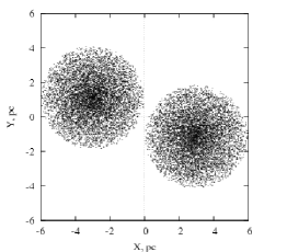
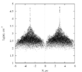
Figure 1: Initial clouds position at $\beta=0.75$.

Firstly, clumps’ centers positioned at $\{-R;\frac{b}{2};0\}$ and $\{R;-\frac{b}{2};0\}$. There are no any internal gas motions in both clumps initially, but they moves to each other along $X$-axis each with velocity $v$ (see Fig. 1 for example).

The mass $\mathfrak{M}$ in both clumps is distributed inside cut-off radius $R$ according to density profile

$$\rho=\frac{\mathfrak{M}}{2\pi R^{2}}\>\frac{1}{r}.$$ (5)

We choose the follow basic parameters for each clump:

$$\mathfrak{M}=2000\,\mathfrak{M}_{\odot},\quad R=3\>\textrm{pc},\quad T=20\>\textrm{K},\quad v=5\>\textrm{km/s},\quad\mu=2.3$$

That is in good agreement with observational data about ISM in our Galaxy [2, 43, 44, 3].

Additionally, each clump have further derived characteristics:

• free-fall time: $\tau_{f\!f}\approx 1.92\>\textrm{Myr}$,

• crossing time: $\tau_{cross}=R/v\approx 0.59\>\textrm{Myr}$,

• isothermal sound speed: $c\approx 0.27\>\textrm{km/s}$,

• mean number density (at given $\mu=2.3$): $\bar{n}\approx 300\>\textrm{cm${}^{-3}$}$,

• ratio of thermal energy to gravitational one: $E_{T}/|E_{G}|\approx 0.09$,

• Jeans’ mass: $\mathfrak{M}_{J}\approx\!1\>\,\mathfrak{M}_{\odot}$ in center and $\approx\!10\>\,\mathfrak{M}_{\odot}$ at edge.

For generation of initial configuration we divide up each clump into $100$ shells of equal mass with boundary radii obeying to density profile (5). Next, we homogeneous and randomly distribute all particles in total number $N$ among this shells in corresponding shares independently for each clump. It is need to note, that then any ideal symmetry was wittingly excluded and there was slight departure in positions of clumps centers from theoretical ones.

The two set of calculations were carried out: one with total number of particles $N=2\!\times\!4000$ and second – with $N=2\!\times\!8000$. In all calculations we used the fixed number of smoothing neighbors $N_{B}=40$, $\alpha_{visc}=0.75$, $\alpha_{toll}=1.00\>\textrm{km/s}$, $\alpha_{C}=0.01$, $\Delta t_{min}=10^{-6}\>\textrm{[t]}$, $\Delta t_{max}=0.75\>\textrm{[t]}$ and gravitation softening $\varepsilon=0.03\>\textrm{ }$ [see 36].

For calculation of all models we had used the supercomputing facilities of Hungarian National Supercomputing Center ​​ (SUN E10k/E15k supercomputers).

4 The Test Runs

Besides main simulations, we first fulfilled a few simple test-runs for study of code characteristics oneself.

First test was adiabatic collapse of cold cloud with density profile (5) and homogeneous specific internal energy distribution

$$u=0.05\frac{G\mathfrak{M}}{R}$$

in natural dimensionless units system $G\!=\!\mathfrak{M}\!=\!R\!=\!1$.

This test, named as ”Evrard-test”, was suggested in Evrard [45] and now became a standard tool for SPH-codes verification [22, 32, 35, 27, 36]. It was calculated out with different particles number $N=(1,2,4,8,16,32)\!\cdot\!10^{3}$ till final moment nearly equal to $3\>\tau_{f\!f}$.

In the full agreement with cited works, at $t\approx 0.7-1\;\tau_{f\!f}$ central bounce was occurred and during outwards shock wave going, significant dissipation of kinetic energy into heat taken place. Nearly at $2.5\;\tau_{f\!f}$ in whole system the virial equilibrium between thermal and potential energies $E_{T}\approx-E_{G}/2$ had been set. Also, test showed the excellent energy conservation $|\delta E/E|<0.1\%$ even at small $N$.

Generally speaking, the total CPU-consumption must determine by selfgravity calculation. Our results showed the typical for TREE-algorithms asymptotic of time consumption $\sim\!O(N\,log(N))$, but the hydrodynamical consumption is even greater then for gravity.

As the next test, we calculated out the spherical isothermal collapse of analogous cloud with mass $\mathfrak{M}=2000\,\mathfrak{M}_{\odot}$, radius $R=3\>\textrm{pc}$, but with temperature $T=20\>\textrm{K}$, as in main simulations. Particles number was set to $N=4000$. After $1.56\,\textrm{Myr}$, that correspond to $0.81\,\tau_{f\!f}$, central dense core with size of $\sim\!0.03\>\textrm{pc}$ was formed close to center ​​ with thin extensive shell around, that have self-similar density distribution $\rho\propto r^{-2}$ [see 46].

The third test was fulfilled for check-up of comparative role of each time-step criterion (3) and (4) and for choice of available accuracy factors. We calculate adiabatic collapse from ”Evrard-test” with $32000$ particles once with fixed $\alpha_{toll}=0.05(G\mathfrak{M}/R)^{1/2}$ and various $\alpha_{C}=0.1,\;0.05,\;0.01,\;0.001$, and another time – the wrong way, with fixed $\alpha_{C}=0.01$ and various $\alpha_{toll}=0.02,\;0.05,\;0.07$. With changing of Courant factor $\alpha_{C}$ the CPU-consumptions was increasing pro rata to its decreasing, that point to determinant role of criterion (4). Since energy error with $\alpha_{C}$ decreasing approach to some limit ($\sim\!0.05\%$), we choose – as a available from ratio accuracy/consumption – its value $\alpha_{C}=0.01$. At such choice, variation of $\alpha_{toll}$ even does not any affect neither on accuracy, nor on time-consumption.

And in the end, we calculate one of clumps collisions – with $N=2\!\times\!4000$, $v=5\>\textrm{km/s}$, $\beta=0.5$ during $1.3\;\textrm{Myr}$ on 1, 2, 4, 8, 16 and 32 SUN UltraSPARC III (1050 MHz) processors for verify of code parallelization. ​​ (see tab. 1)

In general case, any parallel code may be split to so-called consecutive and parallel parts. Therefore it is easy to characterize a quality of code parallelization by relative share of this part in total time-consumption. For example, on parallel part fall

$$\tau_{p}=\frac{1-1/k}{1-1/N_{p}},$$

where $N_{p}$ – processors number, $k>1$ – ratio of durations of task work on single CPU and on $N_{p}$ processors. For GADGET this value is greater then 93%. Also, we can evaluate the effectiveness of CPU loading, as $\epsilon=k/N_{p}$ (tab. 1).

5 The Results

Head-on collision ($\beta=0$)         Because of extensively CPU-consumption this model was traced till $2.885\;\textrm{Myr}$ only. However, already at $1\;\textrm{Myr}$ for $N\!=\!2\!\times\!8000$ and at $1.76\;\textrm{Myr}$ for $N\!=\!2\!\times\!4000$ the number density of central object amounted of $4.5\cdot\!10^{10}\,\;\textrm{cm${}^{-3}$}$ and exceeded the ”opacity limit” ($10^{-13}\;\textrm{g cm${}^{-3}$}\cong 2.6\cdot\!10^{10}\,\;\textrm{cm${}^{-3}$}$, see Masunaga & Inutsuka [47]). So, there was no reason to continue simulation in isothermal approximation at last for this object.

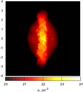
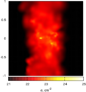
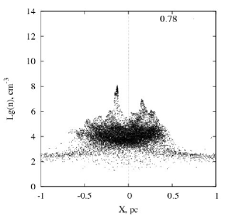
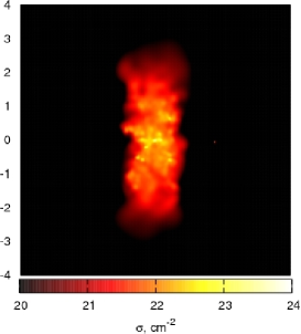
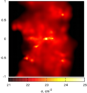
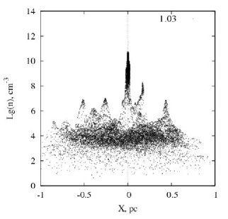
Figure 2: Column-density images along $Z$-axis in large and small scales as well as common logarithms of number density vs. particles $X$-coordinate in model with $\beta=0$. The top row is for time $t=0.78\;\textrm{Myr}$ and the bottom one – for $t=1.03\;\textrm{Myr}$.

The column-density images in $XY$ plane and particles number densities vs. $X$-coordinate on two moment are shown on Fig. 2

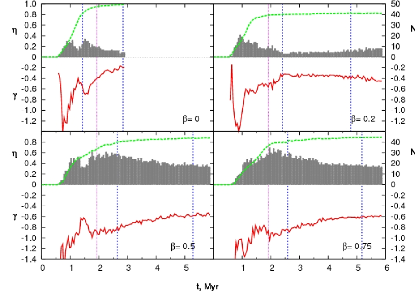
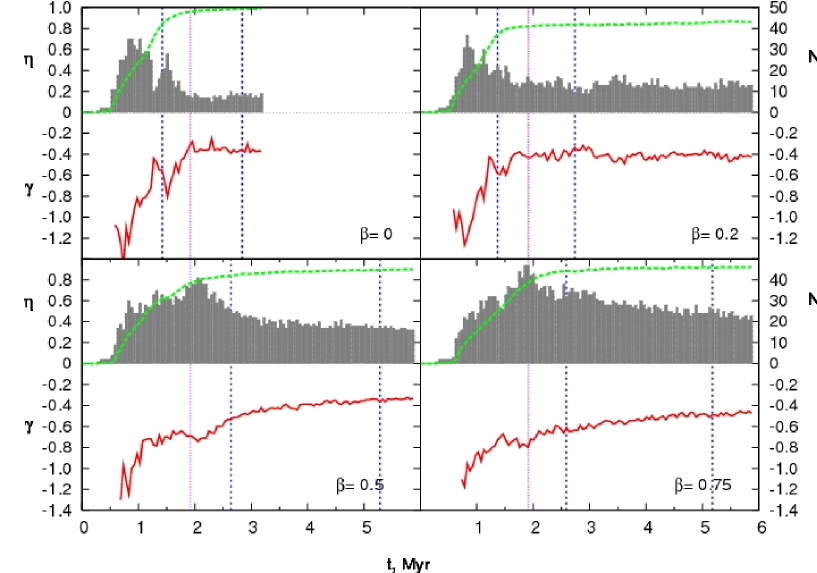
Figure 6: The fragments amount $N_{f}$ (boxes), total fragmentation $\eta$ (dotted line) and slope of fragments mass spectra $\gamma$ (solid line) vs. time for $N\!=\!2\times 4000$ (top) and $N\!=\!2\times 8000$ (bottom). The thin solid vertical line and two dash-dotted lines signs the $\tau_{ff}$, $\tau_{0.8}$ and $2\tau_{0.8}$ moments correspondingly.

Since the collision was going on between the denser clumps centers, the density in shock front had been strong increased and rapid fragmentation there was occurred, that yield the first maximum of fragments amount (see Fig. 6). Next, this fragments began just as rapid merging one with another, giving a few massive central objects (minimum of fragments amount on the same plot). Meanwhile, the rest gas accreting on them, had been compressed and began intensively fragment too, that give the second peak of fragments amount.

Finally, most of gas ($>70\,\%$) fell onto the flatten dense compact core of mass $2921.5\;\,\mathfrak{M}_{\odot}$ and number density up to $6.7\cdot\!10^{11}\,\;\textrm{cm${}^{-3}$}$. There are two non-coplanar discs with masses $537$ and $431.5\;\,\mathfrak{M}_{\odot}$ around this core. The external ring have three small subfragments ($\lesssim 20\;\,\mathfrak{M}_{\odot}$) and entire system are embedded in thin extensive shell with mass $20\;\,\mathfrak{M}_{\odot}$.

The fact of forming of rotational system in head-on case may be explained by features of initial model building (see sec. 3) and therefore there is a small impact parameter close to $0.01\;\textrm{pc}$.

In calculations with half particles number the main picture remain similar to above, but the central body had a one single semi-destroyed most massive accretion disk abounded it. This ”disk” also have one subfragment and entire system was embedded in thin shell.

Collision with $\beta=0.2$         At such small impact parameter clumps’ centers, even if not collided, but passed close enough one from another and collision finished, as above, by forming of one massive zone of fragmentation ​​ in center (the regions in which fragments are formed by groups) and extent, mainly unfragmented diffusive big two-arm spiral with spread in $\sim\!30\;\textrm{pc}$ and thickness from $\sim\!3\;\textrm{pc}$ in center to $\sim\!10\;\textrm{pc}$ on periphery. In contrast to center, each arm consist from gas of its ”own” clump.

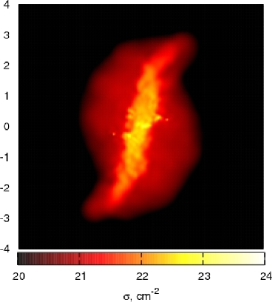
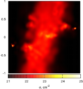
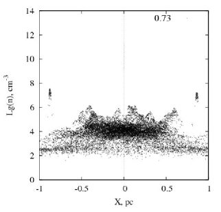
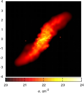
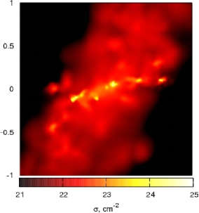
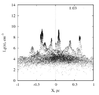
Figure 3: Column-density images with $X-\lg(n)$ plots for $\beta=0.2$. The top row is for time $t=0.73\;\textrm{Myr}$ and the bottom one – for $t=1.03\;\textrm{Myr}$. See notes on Fig. 2

The some moment of evolution are illustrated in Fig. 3. But, at the end of simulated we have the massive flatten core with mass in $1141\;\,\mathfrak{M}_{\odot}$ and number density $\lesssim 1.7\cdot\!10^{10}\,\;\textrm{cm${}^{-3}$}$ in center and its disc-shell by mass $1763.5\;\,\mathfrak{M}_{\odot}$, which oneself have three petty subfragments ($10-15\;\,\mathfrak{M}_{\odot}$). They are surrounded by internal two-armed spiral with size close to $1.5-2\;\textrm{pc}$, that have four fragments ($164.25$, $24$, $16.75$ and $12\;\,\mathfrak{M}_{\odot}$). Rest fragments with masses nearly to $20\;\,\mathfrak{M}_{\odot}$ are detected in both arms of great spiral.

In simulations with $8000$ particles the external spiral was practically unfragmented with the exception of one fragment with mass $22.5\,\mathfrak{M}_{\odot}$.

The core looks like a one-armed spiral of $\sim\!0.75\;\textrm{pc}$ and three satellites with masses in a tens solar masses.

Collision with $\beta=0.5$         At $\beta=0.50$ central clumps’ regions, as before, passed through shock front, has been formed and where at $\sim\!0.6\;\textrm{Myr}$ appeared the first fragments with good mixed gas. Rest material, mainly from outer layers of clumps, go past far from ”place of collision” and form large two-armed spiral structure about of $40\;\textrm{pc}$. The next fragments generation had been formed in outer sided of both arm after $\sim\!1\;\textrm{Myr}$ since extensively fragments formation in shock front.

Now collision gave 4-5 big zones of fragmentation, instead of only one such zone in two previous cases. They are the close pair in center, one single fragment about them and two less massive condensations on the both ends of spiral arms.

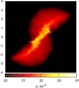
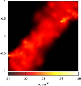
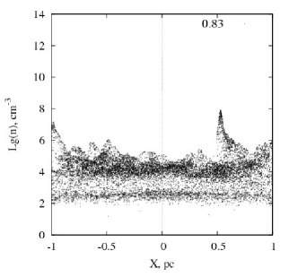
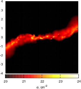
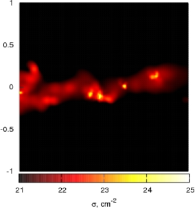
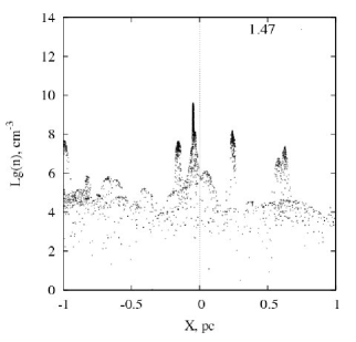
Figure 4: Column-density images with $X-\lg(n)$ plots for $\beta=0.5$. The top row is for time $t=0.83\;\textrm{Myr}$ and the bottom one – for $t=1.47\;\textrm{Myr}$. See notes on Fig. 2

The column-density images and $X$ vs. $Lg(n)$ plots at $0.83$ and $1.47\ ;\textrm{Myr}$ are shown on Fig. 4.

The central pair is two massive flatten cores of masses $563.25$ and $475.5\;\,\mathfrak{M}_{\odot}$ with number densities beyond $10^{9}\;\textrm{cm${}^{-3}$}$, which are surrounded by accretion discs of masses $563.75$ and $610\;\,\mathfrak{M}_{\odot}$, correspondingly and by order less dense. But, the first core yet have low massive thin flat shell ($23.25\;\,\mathfrak{M}_{\odot}$) around, and second one continuously (without space) transform to their disc-shell.

In vicinity of central pair there is a third smaller dense fragment with mass $351.5\;\,\mathfrak{M}_{\odot}$ and number density $\lesssim 2.7\cdot\!10^{9}\,\;\textrm{cm${}^{-3}$}$.

There are core $399.75\;\,\mathfrak{M}_{\odot}$, $(n\lesssim 1.5\cdot\!10^{9}\,\;\textrm{cm${}^{-3}$})$ with double-shell of $73.75\;\,\mathfrak{M}_{\odot}$ on the end of one arm, and another one $382.75\;\,\mathfrak{M}_{\odot}$, $(n\lesssim 8.9\cdot\!10^{8}\,\;\textrm{cm${}^{-3}$})$ with shell in $54.5\;\,\mathfrak{M}_{\odot}$ on the other side.

As for calculations with half mass resolution, in the first place spiral arms are mainly non-fragmented, also, both central core have accretion discs and surrounded by thin flat shells.

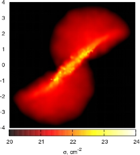
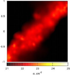
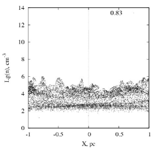
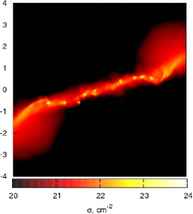
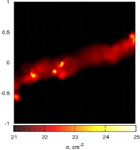
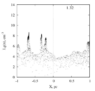
Figure 5: Column-density images with $X-\lg(n)$ plots for $\beta=0.75$. The top row is for time $t=0.83\;\textrm{Myr}$ and the bottom one – for $t=1.32\;\textrm{Myr}$. See notes on Fig. 2

Collision with $\beta=0.75$   (see fig. 5 for illustration)         This is largest impact distance we was considered. In difference from all previous models, now clumps’ centers passed edgeways through forming shock front. Therefore, at chosen clumps velocities and such wide impact parameter the whole collision yield the greatest fragments amount, but with lesser degree of gas mixing since main shaking take place just in shock front.

As before, first intense formation of fragments appeared at $\sim\!0.65\;\textrm{Myr}$ in the shock front and the second fragments generation had been forming in outer side of both lengthy arms $\sim\!0.9\;\textrm{Myr}$ later. But soon, almost all fragments and other gas go far from place of their ”birth”, so that the nearest to center fragments, which are found on about $6\;\textrm{pc}$ from center, are relatively massive dense disc with $\mathfrak{M}=414\;\,\mathfrak{M}_{\odot}$, $n\lesssim 1.1\cdot\!10^{9}\,\;\textrm{cm${}^{-3}$}$ and smaller core in $51.5\;\,\mathfrak{M}_{\odot}$ with shell. The rest fragments have larger remoteness of $16-17\;\textrm{pc}$ from center.

On both ends of extent structure are concentrated by about $1500\,\mathfrak{M}_{\odot}$ in fragments. There are core in $759.25\;\,\mathfrak{M}_{\odot}$ ($n\lesssim 4.8\cdot\!10^{9}\,\;\textrm{cm${}^{-3}$})$ with small shell of $54.15\;\,\mathfrak{M}_{\odot}$. On the another end we have pair of massive fragments groups too: two dense cores with masses $188.25$ and $614\;\,\mathfrak{M}_{\odot}$ with shells in $591$ and $71.75\;\,\mathfrak{M}_{\odot}$ correspondingly. Besides there are yet a few smaller fragments here with masses less then $40\,\mathfrak{M}_{\odot}$ scattered around.

In simulations with worst mass resolution we have more poor fragmentation, but in other respects after all, there are lesser qualitative distinctions between simulations results for $N=2\!\times\!4000$ and $N=2\!\times\!8000$, then in three previous models.

6 Discussion.

At chosen clumps parameters, their masses significantly exceed Jeans’ mass, hence they are gravitationally unstable. Theoretically each clump, taken separately, will collapse out during free-fall time-scale and all fragments, formed under contraction, in the end will have fallen onto the central object. But picture had been radically changed, if both clumps collide rapid enough one with another, so that collision time is lesser then free-fall time (in our models $\tau_{cross}\!:\!\tau_{f\!f}=1\!:\!3$). Now, the evolution of forming fragments will depend from initial impact parameter $\beta$ or (that is same) from initial angular moment of whole system.

In spite of $\beta$ varying in a wide range (and independently from $N$) in all models began intensive gas fragmentation after nearly $\tau_{cross}$ from start of collision, that is in good agreement with such previous work as Gittins et al. [18] and Bhattal et al. [17]. The number density at this time never exceed opaque limit in $\sim\!2.6\cdot\!10^{10}\,\;\textrm{cm${}^{-3}$}$ (see sec. 1); hence the isothermal approximation is quite available, at last, during this period [see 46, 47].

Some general information about gas fragmentation is given in tab. 2. But it is necessary to note here, that owing to improvement of resolution, with invariable SLR and $N_{min}$ (see sec. 2.2) at greater particles number $N$ fragments will be detect earlier and in a larger amounts, then in models with the worst resolution. Therefore, in the tab. 2 are given moments of begin intensive fragmentation in frontier shock front forming during collision, instead of time of first fragments detection.

Since we have carried out comparatively low-resolution modeling we concentrate in this article mainly on integral characteristics of system. The main attention we devoted to the general properties of fragmentation – mass spectra of condensation, their mass share in whole system, etc.

There is a clear correlation between impact parameter $\beta$ and quote of remained fragments to its maximal quantity during evolution: $\kappa\equiv N_{final}/N_{max}\propto\beta$ (see tab. 2). This hint at interclumps collisions may play role not only as a trigger mechanism in ISM fragmentation/starformation, but also as stabilizer of formed fragments system and set the rate of this processes.

We was not built simple, traditional differential mass function, since they showed most sensitiveness to chosen mass interval, quantity of fragments and so, then cumulative one.

The integral mass spectrum can be derived from differential one by its integration either in bounds $(0,m)$, that give the cumulative mass function $N(<m)$, i.e. the quote of fragments with masses less $m$, or in bounds $(m,\infty)$, give the inverse cumulative function $N(>m)$ – the quote of fragments with masses greater then $m$. If differential distribution $\frac{dN}{dm}$ is approached by generally accepted power law $\frac{dN}{dm}=km^{-\alpha}$ ($k,\alpha\!=\!\textrm{{Const},}\;\alpha\!>\!0$), then we have

$$N(<m)=\int\limits_{0}^{m}\frac{\mathrm{d}N}{\mathrm{d}\xi}\mathrm{d}\xi=\frac{k}{1-\alpha}m^{1-\alpha}+c,$$

(where $c=$ is constant, connected with minimal fragments mass) and

$$N(>m)=\int\limits_{m}^{\infty}\frac{\mathrm{d}N}{\mathrm{d}\xi}\mathrm{d}\xi=-\frac{k}{1-\alpha}m^{1-\alpha},$$

where we had taken into account, that $N(>m)$ is a decreasing function ​​.

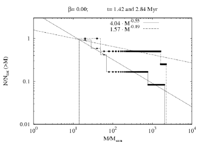
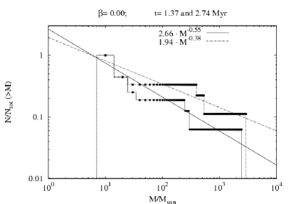
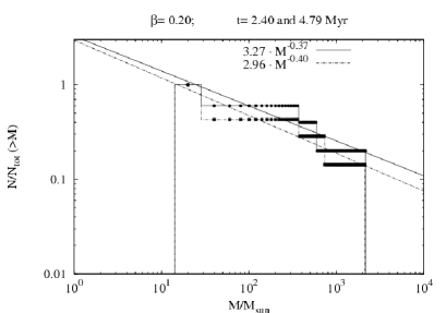
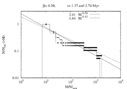
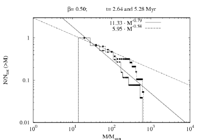
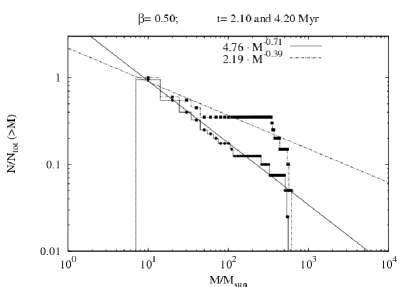
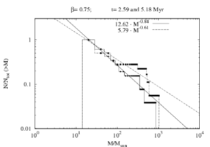
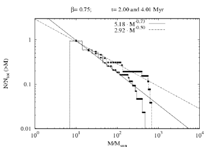
Figure 7: The inverse cumulative mass spectrum for models with $N\!=\!2\times 4000$ (left) and $N\!=\!2\times 8000$ (right). Solid lines for time moment $\tau_{0.8}$ and dotted – for $2\tau_{0.8}$

Since we have not a many data points in our spectra, we choose the inverse cumulative function $N(>m)\equiv 1-N(<m)\propto m^{-\gamma}\;(\gamma>0)$ for data fitting, as it have only two free parameters, instead three ones in another variant and may be linearized by transform to $log$-variables before fitting. The obtained mass function are given on Fig. 7, and their slopes are summarized in tab. 2  ​​.

The trace of fragments amount and total fragmentation index $\eta$ (that we defined as ratio of all fragments mass to mass of whole system: $\eta\equiv\mathfrak{M}_{f}/\mathfrak{M}$) for all evolutionary sequences are given on Fig. 6 together with slopes $\gamma$ of fragments mass spectra. Above all, it is clearly seen the great similarity of curves at the same $\beta$ for both $N$, with the exception of differences in fragments amount on behalf of better resolution and limit values of $\gamma$. Also, it is seen, that always fragments amounts firstly strongly increase during about $0.5-0.6\;\textrm{Myr}$ at $\beta=0,\;0.2$ and $\!\sim\!1.5\;\textrm{Myr}$ at $\beta=0.5,\;0.75$ up to its maximum but next begin decrease, moreover at small $\beta=0.00,0.20$ most rapid, then in two other cases. As to the total fragmentation $\eta$, it rapid increase together with fragments amount, and next its grow practically stopped, not changing to decreasing.

This fact may be explained as that intensive gas disintegration begin at nearly $\tau_{cross}$ and next had been broken out after a time about $1.5-2\;\textrm{Myr}$. But existing fragments continue stick one with another and accrete surrounding gas. Apart from this, the great fragmentation was being achieved at larger impact parameters, with one exception of head-on collision, that gave mainly total fragmentation.

Finally, we had built the dependence of cumulative mass functions slope vs.time for each calculated model, that is present on Fig. 6 by solid line.

As it seen, $\gamma$ smooth rush to certain limit, that is $-0.5...-0.6$ in models with $N=2\times 4000$ and close to $-0.4$ in models with $N=2\times 8000$.

But, since $\gamma$ is continual vary and admissible of our isothermal approximation is restricted in time, we must dwell on some ”typical” its values for represents of our results and comparisons of mass spectra slopes between different models. It is naturally to tie up the typical $\gamma$ with certain typical time moments in connection with process of fragmentation. We chose two such benchmark moments – $\tau_{0.8}$, when $80\%$-fragmentation is reached, and $2\tau_{0.8}$ (Fig. 7).

When 80% of gas got to fragments the mass spectra slopes are nearly $0.5$ for first two models with $\beta=0,\;0.2$ and $0.7$ for two other models (with estimate error less then $\pm 0.03$). After yet $\tau_{0.8}$ period the difference between slopes for collisions with various $\beta$ had been rub off, all spectra became flatten and amount to $\!\sim\!0.4-0.6$.

The resulting slopes of mass spectra are in good agreement with many observational data for molecular clouds and clumps in our Galaxy, especially for large collisions with $\beta=0.5,\;\textrm{and}\;0.75$. Thus, Casoli et al. [8] give $\gamma=0.59$ for $250$ clumps with masses from $4\cdot\!10^{2}\,$ to $2\cdot\!10^{5}\,$ in Perseus arm. Simon et al. [48] from FCRAO and Milky Way Galactic Ring Survey in ¹³CO spectral line received $\gamma=0.80\pm 0.10$ for central Galaxy region; Heyer, Carpenter & Snell [49] from FCRAO Outer Galaxy Survey in lines ¹²CO/¹³CO received $\gamma=0.80\pm 0.03$; Tatsematsu et al. [50] from CS$(1\!-\!0)$ emission for Orion A GMC gave slope $0.6\pm 0.3$; Stutzki & Güsten [5] by analysis of high-resolution maps of M17 SW in C¹⁸O(2-1), C³⁴S(2-1) and C³⁴S(2-1) lines calculated $\gamma=0.72\pm 0.15$; Kramer et al. [11] for seven molecular clouds (also including M17 SW with the same slope) found mainly similar slopes $\gamma=0.6-0.8$ in a wide mass range $10^{-4}-10^{4}\,\mathfrak{M}_{\odot}$;

In spite of not great number of models (in all four) they have divided onto two types with different characteristics – collisions with small and large impact parameter ($0-0.2$ and $0.5-0.75$, correspondingly). In first group, owing to insufficient initial angular moment, there are single dominated by mass center of fragmentation with more or less developed satellites system, spirals etc have been formed. The fragments amount, rapid decrease, after its maximum, but mass distribution slopes are $\!\sim\!0.5$ after $\tau_{0.8}$ and $\!\sim\!0.4$ after twice period.

Another group – collisions with large $\beta$ – lead to form essentially more advanced set of fragments. Now there are a few nearly equivalent centers of fragmentation, so each of they have its own mass dominant component and several satellites. The fragments amount curves are more flatten and mass distribution are steepen: $0.7-0.8$ and $0.5-0.6$ on moments $\tau_{0.8}$ and $2\tau_{0.8}$ correspondingly.

7 Conclusions.

The main our results are follow.

1. After nearly $\tau_{cross}$ after start of collision in all models begin intensive gas fragmentation. The fragment quantity rapid increase up to its maximal value during about $0.5\;\textrm{Myr}$ at $\beta=0,\;0.2$ and $\!\sim\!1.5\;\textrm{Myr}$ at $\beta=0.5,\;0.75$. Next, existing fragments continue stick one with another, but mainly no more fragments formed. Owing to this fact fragments amount decrease (more smooth at lager $\beta$), but their total mass share stay almost constant, from now.

2. With the exception of head-on collision, the total gas fragmentation $\eta$ increase proportional to initial impact parameter. But, at that time the maximal degree of fragmentation ($>98.6\%$) had been reached in head-on case.

3. The quote of remained fragments to its maximal quantity during evolution $\kappa$ is direct proportional to impact parameter, what mean that clouds/clumps collisions may play role not only as a trigger mechanism in ISM fragmentation, but also as stabilizer of formed fragments system.

4. Finally, obtained mass spectra of fragments, that have typical slopes $0.5-0.7$ (see above) accord with many observational data about clouds and clumps in the Galaxy. The mass spectra became flatten with time, but steepens with impact parameter (in time range $[\tau_{0.8};2\tau_{0.8}]$). The difference between two type of collision had been rub off during second $\tau_{0.8}$ period (from $\tau_{0.8}$ to $2\tau_{0.8}$) and was set to $0.4-0.6$.

8 Acknowledgments.

Authors acknowledge the Ukrainian Fund of Fundamental Research for support by grant 02. 07. 00132. The numerical calculations were carried out on SUN E10k/E15k supercomputers in Hungarian National Supercomputing Center (NIIF). In connection with that P. Berczik acknowledge the NIIF for support and given machine time. Authors would like to special thank our colleague Tamas Maray from NIIF for his prolonged assistance in computers using.

P. Berczik wish to express his thanks for the support of his work to the German Science Foundation (DFG) under SFB439 (sub-project B11) ”Galaxies in the Young Universe” and (computer hardware) by ”Volkswagenstiftung” (Project GRACE).

Also, authors acknowledge S. G. Kravchuk from MAO for useful remarks and discussion of our results.

$N_{proc}$	$N_{step}$	$t_{total}$	$t_{grav}$	$t_{hydro}$	$speed$	$\tau_{p}$	$\epsilon$
1	177,482	17,461.27	6,455.20	10,285.22	10.164	—	—
2	167,882	9,254.15	3,778.87	5,033.96	18.141	0.940	0.943
4	164,704	5,059.01	1,903.46	2,723.69	32.557	0.947	0.863
8	168,956	2,741.42	925.20	1,549.85	61.631	0.963	0.796
16	167,245	2,170.76	630.79	1,269.27	77.044	0.934	0.503
32	169,125	2,346.10	570.27	1,328.61	72.088	0.894	0.233

Table 1: CPU consumptions for test. $N_{proc}$– CPUs number (SUN UltraSPARC III 1050 MHz), $N_{step}$– time-steps number, $t_{total}$– the total time consumption on whole task in seconds, $t_{grav}$– time consumptions on gravity calculation (including tree-building) in seconds, $t_{hydro}$ – the same on hydrodynamics (including neighbors search), $speed$ – the total calculation speed in sps (steps per second), $\tau_{p}$ – the share of parallel part of code in $t_{total}$, $\epsilon$ – the effectiveness of CPUs loading (see text).

	begin fragmentation				end of simulation						$\gamma$
$\beta$	$\tau$	$n_{max}$	$N_{f}$	$\mathfrak{M}_{f}$	$\tau$	$n_{max}$	$N_{f}$	$\mathfrak{M}_{f}$	$\eta$	$\kappa$	$\tau_{0.8}$	$2\tau_{0.8}$
$N=2\!\times\!4000$
0.00	0.59	$4.68\cdot\!10^{5}\,$	1	114.5	2.89	$4.68\cdot\!10^{12}\,$	4	3945.0	0.986	0.257	0.55	0.19
0.20	0.59	$5.20\cdot\!10^{5}\,$	2	107.0	5.87	$2.13\cdot\!10^{10}\,$	8	3304.0	0.826	0.351	0.37	0.40
0.50	0.59	$4.94\cdot\!10^{5}\,$	1	21.0	5.87	$1.14\cdot\!10^{11}\,$	17	3519.0	0.880	0.390	0.79	0.58
0.75	0.64	$1.04\cdot\!10^{5}\,$	1	26.5	5.87	$4.16\cdot\!10^{9}\,$	17	3578.5	0.895	0.489	0.84	0.61
$N=2\!\times\!8000$
0.00	0.54	$3.70\cdot\!10^{7}\,$	11	244.50	2.89	$6.68\cdot\!10^{11}\,$	9	3943.75	0.986	0.235	0.55	0.38
0.20	0.49	$1.68\cdot\!10^{7}\,$	3	41.25	5.87	$1.65\cdot\!10^{10}\,$	13	3451.50	0.863	0.381	0.52	0.43
0.50	0.54	$3.30\cdot\!10^{7}\,$	4	59.75	5.87	$8.98\cdot\!10^{10}\,$	16	3600.50	0.900	0.548	0.71	0.39
0.75	0.59	$3.46\cdot\!10^{7}\,$	3	48.50	5.87	$9.44\cdot\!10^{9}\,$	23	3698.25	0.925	0.486	0.73	0.50

Table 2: The parameters of fragmentation for models with both $N$. $\tau$– time in Myr, $n_{max}$– the maximal number density (in cm^-3) at this moment, $N_{f}$– fragments amount in system, $\mathfrak{M}_{f}$ – mass of all fragments in $\,\mathfrak{M}_{\odot}$, $\eta$– system fragmentation, $\kappa$– the quote of remained fragments to its maximal quantity, $\tau_{0.8}$– the moment, when $80\%$-fragmentation is reached, $\gamma$– the integral mass function slope ($dN/dm\propto m^{-\gamma}$).

References

- Bochkarev [1981] Bochkarev N. G. Mezhzvyozdnaya sreda i zvezdoobrazovanie // Zvyozdi i zvyozdnie sistemi/Pod red. D. Ya. Martinova – M.:Nauka, 1980 – P.265–325.
- Shu et al. [1987] Shu F. H., Adams F. C., Lizano S. Star formation in molecular clouds: observation and theory // ARA&A. – 1987. – 25. – 23–81.
- Ferrière [2001] Ferrière K. M. The interstellar environment of our Galaxy // Review of Modern Physics. – 2001. – 73,N4. – 1031–1066. (astro-ph/0106359)
- Motte et al. [1998] Motte F., André P., Neri R. The initial conditions of star formation in the Ophiuchi main cloud: wide–field millimeter continuum mapping // A&A. – 1998. – 336. – 150–172.
- Stutzki & Güsten [1990] Stutzki J., Güsten R. High spatial resolution isotopic CO and CS observations of M17 SW: The clumpy structure of the molecular cloud core // ApJ. – 1990. – 356. – 513–533.
- Arshutkin & Kolesnik [1990] Arshutkin L. N., Kolesnik I. G. Stroenie molekulyarnikh oblakov // Stroenie i evolyutziya oblastej zvezdoobrazovaniya /Pod red. I. G. Kolesnika – Kiev:Naukova Dumka, 1990 – P.103–160.
- Larson [1981] Larson R. B. Turbulence and star formation in molecular clouds // MNRAS. – 1981. – 194. – 809–826.
- Casoli et al. [1984] Casoli F., Combes F., Gerin M. Observation of molecular clouds in the second galactic quadrant // A&A. – 1984. – 133,N1. – 99 – 109.
- Stark [1984] Stark A. A. Kinematics of molecular clouds. I. Velocity dispersion in the solar neighborhood // ApJ. – 1984. – 281,N2. – 624–633.
- Elmegreen [1985] Elmegreen B. G. Molecular clouds and star formation: an overview // Protostars and Planets II / eds. D. C. Black and M. Sh. Matthews – University of Arizona Press, 1985. – P.33 – 58.
- Kramer et al. [1998] Kramer C., Stutzki J., Röhrig R. Corneliussen U. Clump mass spectra of molecular clouds // ApJ. – 1998. – 329. – 249–264.
- Das & Jog [1996] Das M., Jog C., J. Collisional buildup of molecular clouds: mass and velocity spectra // ApJ. – 1996. – 462. – 309–315.
- Lattanzio & Henriksen [1988] Lattanzio J. S., Henriksen R. N. Collisions between rotating interstellar clouds // MNRAS. – 1988. – 232. – 565–614.
- Lattanzio et al. [1985] Lattanzio J. S., Monaghan J. J., Pongracic H., Schwartz M. P. Interstellar cloud collisions // MNRAS. – 1985. – 215. – 125–147.
- Monaghan & Varnas [1988] Monaghan J. J., Varnas S. R. The dynamics of interstellar cloud complex // MNRAS. –1988. – 231. – 515–534.
- Marinho & Lépine [2000] Marinho E. P., Lépine J. R. D. SPH simulations of clumps formation by dissipative collision of molecular clouds // A&A. Suppl. Ser. – 2000. – 142. – 165–179.
- Bhattal et al. [1998] Bhattal A. S., Francis N., Watkins S. J., Withworth A. P. Dynamically triggered star formation in giant molecular clouds // MNRAS. – 1998. – 297,N2. – 435 – 448. (astro-ph/9805001)
- Gittins et al. [2003] Gittins D. M., Clarke C. J., Bate M. R. Hydrodynamical simulations of a cloud of interacting gas fragments // MNRAS. – 2004. – 340,N3. – 841–850. (astro-ph/0301136)
- Bate et al. [1995] Bate M. R., Bonnell I. A., Price N. M. Modelling accretion in protobinary systems // MNRAS. – 1995. – 277,N2. – 362 – 376.
- Lucy [1977] Lucy L. B. A numerical approach to the testing of the fussion hypothesis // AJ. – 1977. – 82. – 1013–1024.
- Gingold & Monaghan [1977] Gingold R. A., Monaghan J. J. Smoothed particle hydrodynamics: theory and application to non–spherical stars // MNRAS. – 1977. – 181. – 375–389.
- Hernquist & Katz [1989] Hernquist L., Katz N. TREESPH: A unification of SPH with the hierarchical tree method // ApJS. – 1989. – 70. – 419–446.
- Berczik [1999] Berczik P. Chemo–dynamical smoothed particle hydrodynamics code for evolution of star forming disk galaxies // A&A. – 1999. – 348. – 371–380.
- Berczik [2000] Berczik P. Modeling the star formation in galaxies using the chemo-dynamical SPH code // A&SS. – 2000. – 271. – 103–126.
- Berczik et al. [2003] Berczik P., Hensler G., Theis Ch., Spurzem R. A multi-phase chemo-dynamical SPH code for galaxy evolution. Testing the code // A&SS. – 2003. – 284. – 865–868.
- Spurzem et al. [2004] Spurzem R., Berczik P., Hensler G., Theis Ch., Amaro-Seoane P., Freitag M., Just A. Physical Processes in star-gas systems // PASA. – 2004. – 21. – 1–4.
- Carraro et al. [1998] Carraro G., Lia C., Chiosi C. Galaxy formation and evolution. I. The Padua TREE–SPH code (PD–SPH) // MNRAS. – 1998. – 297,N4. – 1021 – 1040.
- Monaghan [1992] Monaghan J. J. Smoothed particle hydrodynamics // ARA&A. – 1992. – 30. – 543–574.
- Berczik & Kolesnik [1993] Berczik P. P., Kolesnik I. G. Sglazhivaemaya gidrodinamika chastitz i eyo primenenie dlya resheniya astrofizicheskikh problem // KFNT. – 1993. – 19,N2. – 3–14.
- Hiotelis & Voglis [1991] Hiotelis N., Voglis N. Smooth particle hydrodynamics with locally readjustable resolution in the collapse of gaseous protogalaxy // A&A. – 1991. – 243. – 333–340.
- Lombardi et al. [1999] Lombardi J. C., Sills A., Rasio F. A., Shapiro S. L. Test of spurious transport in smoothed particle hydrodynamics // J. Comp. Phys. – 1999. – 152. – 687.
- Thaker et al. [2000] Thaker R. J., Tittley E. R., Pearce F. P., Couchman H. M. P., Thomas P. A. Smoothed particle hydrodynamics in colsmology: a comparative study of implementation // MNRAS. – 2000. – 319. – 619.
- Berczik & Kolesnik [1998] Berczik P., Kolesnik I. G. Gasodynamical model of the triaxial protogalaxy collapse // Astronomical and Astrophysical Transactions. – 1998. – 16. – 163–185.
- Monaghan & Lattanzio [1985] Monaghan J. J., Lattanzio J. C. A refined particle method for astrophysical problems // A&A. –1985. – 149. – 135–143.
- Steinmetz & Müller [1993] Steinmetz M., Müller E. On the capabilities and limits of smoothed particle hydrodynamics // A&A. – 1993. – 268. – 391–410.
- Springel et al. [2001] Springel V., Yoshida N., White S. D. M. GADGET: a code for collisionless and gasdynamical cosmological simulations // New Astronomy – 2001. – 6. – 79–117.
- Burnes & Hut [1986] Burnes J. E., Hut P. A hierarchical force-calculation algorithm // Nature. – 1986. – 324. – 446.
- Huchra & Geller [1982] Huchra J. P., Geller M. J. Groups of galaxies I. Nearby groups // ApJ. – 1982. – 257. – 423–437.
- Frederic [1994] Frederic J. J. Testing the accuracy of redshift space grown finding algorithms // ApJS. – 1995. – 97,N2. – 259–274. (astro-ph/9409015)
- Botzler et al. [2003] Botzler C. S., Snigula J., Bender R., Hopp U. Finding structures in photometric redshift galaxy surveys: An extended friends-of-friends algorithm // MNRAS. – 2004. – 349,N2. – 425–439. (astro-ph/0312018)
- Davies et al. [1985] Davies M., Efstathiou G., Frenk C. S., White S. D. M. The evolution of large–scale structure in a universe dominated by cold dark matter // ApJ. – 1985. – 292,N2. – 371–394.
- Burnes & Efstathiou [1987] Burnes J., Efstathiou G. Angular momentum from tidal torques // ApJ. – 1987. – 319,N2. – 575–600.
- Williams et al. [1999] Williams J. P., Blitz L., McKee C.F. The structure and evolution of molecular clouds: From clumps to cores to the IMF // Protostars and Planets IV / eds. V. Mannings, A. P. Boss, S. S. Russell – University of Arizona Press, 2000. (astro-ph/9902246)
- Blitz & Williams [1999] Blitz L., Williams J. P. Molecular clouds // The Origin of stars and Planetary Systems / ed. C. L. Lada and N. D. Kylafis – Kluwer Academic Publishers, 1999. (astro-ph/9903382)
- Evrard [1988] Evrard A. E. Beyond N–body – 3D cosmological gas dynamics // MNRAS. – 1988. – 235 – 911–934.
- Larson [1969] Larson R. B. Numerical calculation of the dynamics of a collapsing protostar // MNRAS. – 1969. – 145. – 271–295.
- Masunaga & Inutsuka [2000] Masunaga H., Inutsuka S. A radiation hydrodynamic model for protostellar collapse: II. The second collape and the birth of a protostars // ApJ. – 2000. – 531. – 350–365.
- Simon et al. [2001] Simon R. et al. The structure of four molecular cloud complexes in the BU-FCRAO Milky Way galactic ring survey // Astrophys.J. – 2001. – 551. – P.747–763.
- Heyer, Carpenter & Snell [2001] Heyer M. H., Carpenter J. M., Snell R. L. The equilibrium State of molecular regions in the outer Galaxy // ApJ. – 2002. – 578. – 229–244. (astro-ph/0101133)
- Tatsematsu et al. [1993] Tatsematsu K. et al. Molecular cloud cores in the Orion A cloud. I. Nobeyama CS (1-0) survey // ApJ. – 1993. – 404. – 643–662.