GEOMETRIC MODEL OF QUINTESSENCE

V. Folomeev, V. Gurovich † and I. Tokareva ‡

†

Physics Institute of NAN KR, 265 a, Chui str., Bishkek, 720071, Kyrgyz Republic

‡

Physics Department, Technion, Technion-city, Haifa 32000, Israel

On basis of modification of Einstein’s gravitational equations by adding the term $f(R)\propto\beta R^{n}$, a geometric model of quintessence is proposed. The evolution equation for the scale factor $a$ of the Universe is analyzed for the two parameters $n=2$ and $n=4/3$, which were preferred by previous studies of the early Universe. Another choice of parameters $n$ and $\beta$ is proposed from the following reasons: the exponent $n$ close to $1.2953$ follows from the request for the evolution of the Universe after recombination to be close to the evolution of the flat FRW model with cold dark matter and reasonable age of the Universe defines the value of the coefficient $\beta$. Such a model corresponding to the evolution of the Universe with the dynamical $\Lambda$-term describes well enough the observational data.

1. Introduction

The discovery of accelerated expansion of the Universe [1, 2, 3] has stimulated the quest for mechanism of present inflation. The most famous theoretical model of dark energy (DE) is the cosmological constant $\Lambda$. The corresponding FRW solution for flat Universe with the present densities ratio for cold matter and dark energy ($\Omega_{m}/\Omega_{\Lambda 0}\sim 0.3/0.7$) describes satisfactorily the evolution of the Universe at low redshifts [3, 4, 5]. However, the nature of the constant $\Lambda$-term has been remaining to be inexplicable during many years.

It is well-known, the application of the constant $\Lambda$-term for modeling of the early Universe was initially confronted with principal difficulties. Solving the problems of the very early Universe, this term has to be reducing by several order of magnitude during following evolution of the Universe. This problem was solved by rejection of $\Lambda$-term, and corresponding inflationary behavior was determined by models of “effective $\Lambda$-term” - quasi-classical scalar fields in the one way. The progress of these models is well-known. Another way to describe the inflationary behavior is to take into account the polarization of vacuum of quantum fields in the early Universe. Taking into account of the effects of polarization leads to appearance of the terms non-linear on curvature in the Einstein-Hilbert action. In such models the inflation appears self-consistently. Let us note two issues:
- a correction to the Einstein-Hilbert action with an arbitrary function of scalar curvature $R$ is equivalent mathematically to the introduction of scalar field into the classical Friedmann cosmology [5, 6, 7, 8];
- the terms of the form $R^{n}$ were investigated in the early works done on the problem of singularity before obtaining of exact corrections to the Einstein action following from the one loop approximation [9]. The part of such solutions approaches asymptotically to the Friedmann solutions with $\Lambda$-term, however physical results of the solutions have not been explained at that time.

For the purpose to explain the accelerated expansion of the Universe today, it is naturally to use the experience cumulative at investigations of the early Universe. Thus, one of the tendencies is concerned with the hypothesis of existence some scalar fields that determine the density of dark energy (see e.g. [10, 11, 12]). The another tendency models is an effective quasi-hydrodynamical energy-momentum tensor describing the observational data [13]. And the third tendency consists in generalization of the Einstein-Hilbert equation by inclusion of curvature invariants [14, 15, 16] analogously to the earlier works mentioned above. The last approach one can consider to be either an independent approach to describing of DE or an analogue of inclusion of scalar fields (in case of $f(R)$) as stated above.

In the works on the higher order gravity theories (HOGT), the models with power corrections were investigated, however they have never been fitted to whole set of the observational data.

In this paper, the model with correction $f(R)\propto R^{n}$ with $n>0$ is considered in detail for the purpose to correlate it with the observational data. In the other words, we would like to obtain the model that does not conflict with the scenario of the large scale structure formation (in past) and describes satisfactorily the Universe undergoing an accelerated expansion at present. Therefore, at the minimum, within the framework of the $f(R)$-theories, we will obtain solutions remind $\Lambda$CDM model describing well enough by set of the observational data [3, 4]. However, as it was mentioned by various authors (see [5] and references therein), the observational data indicates the models of dynamical DE. Hence, our second aim is to search out such dynamical solutions within the framework of HOGT and to find out whether these solutions are preferable.

This paper is organized as follows. In section 2 the basic equations of HOGT are presented. Section 3 is devoted to consideration of the models with $n=2$ and $n=4/3$. In section 4 for the corrections of the form $f(R)\propto\beta R^{n}$ we find the exponent $n_{1}=1.2953$ which allows generalization of the Einstein equation for the scale factor $a$ to have a particular solution corresponding to the flat FRW solution for cold matter. We show that instability of the solutions, that are close to this particular solution at $z\gg 1$, may lead to the accelerated behavior of the model at present and the following asymptotic approach of the solution to the solution with the constant $\Lambda$-term. In section 5 we discuss our results and compare them to observations. In the model there are only two free parameters - the coefficient $\beta$ and a slight deviation of the parameter $n$ from $n_{1}=1.2953$ mentioned above. Fixed from one set of the observational data, they allow to obtain the rest of the set of the observational data.

2. Basic equations

As suggested by observations, we consider the flat cosmological Friedmann model with the metric

$$ds^{2}=d\tau^{2}-a(\tau)^{2}(dx^{2}+dy^{2}+dz^{2}).$$ (1)

If $H_{0}$ denotes the presently observable Hubble constant (the subscript 0 will always indicate the present epoch), the reduced curvature tensor $\rho_{k}^{l}\equiv H_{0}^{-2}R_{k}^{l}$ has the following matrix elements as a function of the reduced time $\theta\equiv H_{0}\tau$, with the notation $\dot{a}\equiv da/d\theta$:

$$\rho_{0}^{0} = -3\ddot{a}/a,$$ (2)

$$\rho_{i}^{i} \equiv \rho=-6\left(\ddot{a}/a+\dot{a}^{2}/a^{2}\right).$$ (3)

The variation of Einstein’s Lagrangian with an additional term $\Delta L(R)\equiv f(R)$ gives

$$G_{i}^{k}=\frac{8\pi G}{H_{0}^{2}}T_{i}^{k}+\hat{T}_{i}^{k};\quad G_{i}^{k}=\rho_{i}^{k}-\frac{1}{2}\delta_{i}^{k}\rho.$$ (4)

Here $T_{i}^{k}$ corresponds only to cold matter in the present Universe and

$$-\hat{T}_{i}^{k} = \left(\frac{\partial f}{\partial\rho}\right)\rho_{i}^{k}-\frac{1}{2}\delta_{i}^{k}f+$$ (5)

$${}\left(\delta_{i}^{k}g^{lm}-\delta_{i}^{l}g^{km}\right)\left(\frac{\partial f}{\partial\rho}\right)_{;l;m}$$

specifies the effective quintessence with the nontrivial dependence on curvature.

We proceed as in Ref. [17] by introducing the new variable

$$y\equiv(\dot{a}a)^{2}$$ (6)

which allows to reduce the order of the equations. Then the $i=k=0$ component of Eq. (4) leads to

$$y+\left[f_{,\rho}\left(y-\frac{a}{2}\frac{dy}{da}\right)-\frac{a^{4}}{6}f(\rho)+ay\frac{df_{,\rho}}{da}\right]=$$ (7)

$$\frac{\rho_{m}}{\rho_{*}}a^{4}\equiv\Omega_{m}a,$$

where $\rho_{m}$ is the $a$-dependent cold dark matter (CDM) energy density, $\rho_{*}=3H_{0}^{2}/8\pi G$ is the critical density. Choosing the value of the scale factor $a(\theta_{0})$ equal to 1 at present, one has $\rho_{m}=\rho_{0}/a^{3}$ and $(\rho_{m}/\rho_{*})a^{4}\equiv\Omega_{m}a$.

In order to investigate the evolution of the cosmological model it is enough to obtain the solution of Eq. (7) with appropriate initial conditions. But for interpretation of the solution and for its comparison with observations it is necessary track for changes of CDM energy density $\rho_{m}$ and quintessence energy density $\rho_{v}$ separately. For this purpose we use $i=k=0$ component of Einstein’s equations (4)

$$G_{0}^{0}=\rho_{0}^{0}-\frac{1}{2}\rho=\frac{8\pi G}{H_{0}^{2}}\left(\rho_{m}+\rho_{v}\right).$$ (8)

Multiplying this equation by $a^{4}$ and using Eqs. (2),(3) and (6), we have

$$y=(\rho_{m}+\rho_{v})a^{4}/\rho_{*}$$ (9)

accounting for the evolution of cold matter energy density. From this we find for the quintessence energy density:

$$\frac{\rho_{v}}{\rho_{*}}=(y-\Omega_{m}a)/a^{4}.$$ (10)

By solving Eq. (7), we can find the evolution of $\rho_{v}$. At known $y$, the Hubble parameter

$$h(a)=\sqrt{y/a^{4}},$$ (11)

the deceleration parameter of the Universe

$$q=-\frac{\ddot{a}a}{\dot{a}^{2}}=\frac{1}{2}\left(1+\frac{3\delta_{v}w}{1+\delta_{v}}\right);\quad\delta_{v}=\rho_{v}/\rho_{m},$$ (12)

and the equation of state

$$w=\left(\frac{2q-1}{3}\right)\left(\frac{\delta_{v}+1}{\delta_{v}}\right).$$ (13)

Here we will investigate corrections to the Einstein-Hilbert action of the form

$$f(R)=-\alpha\,R^{n}.$$ (14)

In such a case, Eq. (7) can be presented in the form

$$\beta\left[n(n-1)y^{\prime\prime}y+\frac{(1-n)}{2}(y^{\prime})^{2}+n(4-3n)\frac{y^{\prime}y}{a}\right]=$$

$$\frac{(y^{\prime})^{2-n}}{a^{4-3n}}(y-\Omega_{m}\,a),\quad$$ (15)

$$\beta=(-3)^{n-1}\alpha.\qquad\qquad\qquad\qquad\qquad\qquad\qquad\quad$$

A general approach to investigation of the last equation is given in [17].

From (2.) we see that a simple power in the asymptotic solutions is absent for $n=2$ and $n=4/3$. These happen to be the same parameters which were of special importance in a previous theory of the early Universe. At $n=4/3$, one of us [9] has obtained for the first time a cosmological model without a singularity. That model passes through a regular minimum, has inflationary stage and tends asymptotically to the classical Friedmann solutions. In addition, the usefulness of an additional term $R^{2}$ in the models of the early Universe has been pointed out before. Therefore we analyze the possibility of using of such powers for construction of models with variable parameters $q$ and $w$.

3. Models with $n=2$ and $n=4/3$

These models have been considered in details in [16]. The model with $n=2$ was often used in the theory of the early Universe. It describes the stage of fast oscillations of $a(\theta)$ (the so called scalaron stage, which was introduced by A. Starobinsky in [18]). The damping of such oscillations was connected with creation of unstable particles and filling of the early Universe by a hot plasma.

Here we want to consider this model in the opposite regime when the period of oscillations is commensurable with age of the Universe $1/H_{0}$. One can easily see the oscillations of the model by inserting the specified form of quintessence in (4) and (5)

$$\frac{d^{2}\rho}{d\theta^{2}}+3\frac{\dot{a}}{a}\frac{d\rho}{d\theta}+(\rho+\Omega_{m}a)=0.$$ (16)

The scalar curvature performs oscillations near the value of $\rho$ which corresponds to the model of cold dust matter in the Friedmann Universe.

The special feature of the model with $n=4/3$ consists in absence of the scale factor $a$ in explicit form in the Einstein’s equations if matter is neglected [9]. This allows one to find the general solution of Eq. (2.) with given $n$. One can show that de Sitter’s solution arises in the limit $a\gg 1$. The curvature of this limiting solution is determined by the parameter $\alpha$.

For a further analysis of these models and comparison with observable data see Section 5.

4. The best-fit model

In Eq. (2.) there are two parameters, $\beta$ and $n$, determined by the observational data. These parameters could be chosen according to different requirements [15, 16]. Here we will choose parameter $n$ from requirement of closeness of evolution of our model to the classical solution for the flat FRW Universe with cold matter in the past [19]. This fact allows this scenario to be close to the scenario of the large scale structure formation. This requirement can be realized at condition that the classical Friedmann solution

$$y=\Omega_{m}\,a$$ (17)

is a particular solution of Eq.(2.). It is easy to see from Eq.(2.), the last condition is equivalent to the choice of $n$ to be satisfying the equation

$$n-1=2n(4-3n)\qquad\qquad\qquad\qquad\qquad\qquad\qquad$$ (18)

with roots

$$n_{1}=1.295,\quad n_{2}=-0.129.$$ (19)

The first of the roots leads to the type of models of papers [15, 16], while the second root corresponds the models with correction of the form $\propto\mu/R^{|n_{2}|}$ investigated in [20]. As it will be shown below, such a choice of $n$ approaches the model to the set of the observational data in the best way.

4.1. Behavior of the dust solution in the $f(R)$-model in past

After recombination, the evolution of the Universe has to be described by the Friedmann model with the cold matter. The dynamics of expansion is determined by stability of the dust solution in the model (2.). If the solution is stable, then the model evolves in the way very close to classical one. However, the observational data at $z<1$ does not correspond to such a scenario, i.e. we are interested in dust-like solutions which are not stable in the model (2.) but the perturbations do not grow catastrophically fast. Otherwise, the model does not provides a sufficiently long period with $q\simeq 0.5$ at $z\gg 1$ required for the large structure formation.

For investigation of behavior of the solution (17) we will search a perturbed solution in the form

$$y=\Omega\,a(1+\psi),\quad\psi\ll 1.$$ (20)

In this linear approximation and close to the recombination time ($a\ll 1$) Eq. (2.) yields,

$$n\,a^{2}\,\psi^{\prime\prime}+a\,\psi^{\prime}(2n-0.5)=0,$$ (21)

with the damping solution $\psi=C_{1}+C_{2}\,a^{(\frac{1}{2n}-1)}$. Hence the solution (17) for the $f(R)$-theory (14) with $n=n_{1}$ satisfying Eq.(18) asymptotically approaches to to the flat FRW solution, i.e. it is stable and does not satisfies the requirement stated above.

As the next step on the path of the choice of $n$, we will look for solutions of the $f(R)$-theories (14) with $n$ which is a little different from $n_{1}$,

$$n=n_{1}+\delta n,\qquad\delta n\ll 1.$$ (22)

It is efficient to rewrite the condition (18) in the form

$$\delta\,(n-1)=2n(4-3n),\quad\delta=1+\epsilon,\quad\epsilon\ll 1.$$ (23)

 

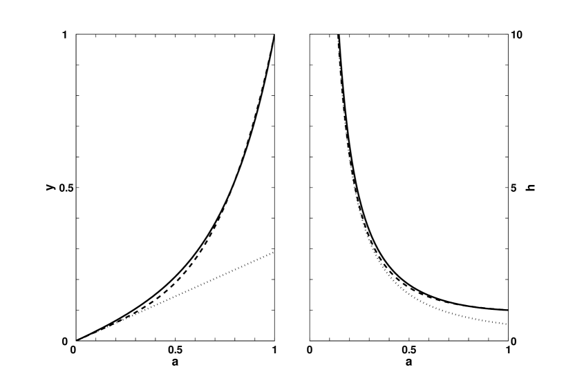
Figure 1: The evolution of the variable $y$ (a left panel) and the Hubble parameter $h$ (a right panel) with the scale factor $a$ are represented by the solid line. The $\Lambda$CDM solution and the cold matter solution are presented by dashed and dotted line, respectively. Both graphs correspond to the case $\Omega_{m}=0.29.$

We will look for the perturbed dust-like solution in the form (20) near to recombination. Eq.(2.) for such a case yields

$$n\,a^{2}\,\psi^{\prime\prime}+2a\,\psi^{\prime}\left(n-0.5+\delta/4\right)+\left(\delta-1\right)=0.$$ (24)

Then after the change of variable $\xi=\ln(a/a_{\ast})$ the Eq. (24) yields

$$n\ddot{\psi}+\left(n-1/2+\epsilon/2\right)\dot{\psi}+\epsilon=0,\,{\bf\dot{}}=d/d\xi.$$ (25)

The last equation has a solution

$$\psi=\left(C_{1}+\frac{2\,\epsilon}{1-2n}\ln\left(\frac{a}{a_{\ast}}\right)\right)+C_{2}\,a^{(\frac{1}{2n}-1)}.$$ (26)

The analysis of (26) has shown that the requirement stated above is realized only for $\epsilon<0$.

In this case, the modification of the exponent (23) is determined by a small positive correction

$$\delta n\simeq-2\,\epsilon\,n_{1}(n_{1}-1)/(12n_{1}-1).$$ (27)

The numerical analysis has shown that behavior of solutions is sensitive to small changes of $\epsilon$ at $a\rightarrow 1$. The last fact together with a choice of parameter $\beta$ allows us to obtain a good enough correspondence with the observational data.

As an illustration we give the results for the set of parameters $n=1.296,\;\beta=0.467$ fixed according to $\Omega_{m}=0.29,h_{0}=68$ (the best fit to the CMB+SNe data presented in [5]). In a left panel of Fig. 1, a solid line represents the evolution of the variable $y$ with the scale factor $a$. At the beginning, it coincides with the evolution of the dust model which is represented by a dotted line but further it deviates to the $\Lambda$CMD model represented by a dashed line. In a right panel, one can see evolution of the Hubble parameter with the scale factor $a$ for the mentioned three models.

4.2. The behavior of the solution in future

The further expansion of the Universe at $a\gg 1$ according to Eq. (2.) leads to the negligible effect of cold matter on the solution behavior. In this case, de Sitter solution $y=\Omega\,a^{4}$ is an asymptotic solution of Eq.(2.). This solution corresponds to the constant Hubble parameter

$$h(a\rightarrow\infty)=\sqrt{\Omega}$$ (28)

with $\Omega$ defined from equality

$$3\beta(2n-1)(n-1)/2=(4\Omega)^{(1-n)}/4$$ (29)

The inflationary solution is stable in the process of evolution of the model. To show it, we shall look for a solution with perturbation in the form
$y=\Omega a^{4}(1+\Phi),\quad\Phi\ll 1$. This ansatz yields

$$n_{1}a^{2}\Phi^{\prime\prime}+[(n_{1}-1)/2+3n_{1}^{2}]a\Phi^{\prime}+$$ (30)

$$6(2n_{1}^{2}-3n_{1}+1)\Phi=0.$$

The change of variable $a$ to variable $\xi$ (see Eq.(26)) yields

$$\ddot{\Phi}+A\dot{\Phi}+B\Phi=0,\quad\dot{}=d/d\xi.$$ (31)

where coefficients are $A=[3n_{1}-(1/n_{1}+1)/2]=2.99$, $B=6(2n_{1}-3+1/n_{1})=2.18$. This equation for perturbations have a damped solution indicating de Sitter solution to be stable. The numerical analysis has shown that de Sitter solution is an attractive solution.

As an example let us consider the evolution of the Hubble parameter for the case $\Omega_{m}=0.29$. In contrast to the Hubble parameter of $\Lambda$CDM model monotonically decreasing down to constant $\sqrt{\Omega_{\Lambda}}$, it reaches a minimum $h_{m}\approx 0.978$ at $a\approx 1.15$ and after that increases up to the asymptotic solution (28). It is interesting to note that the formula for the dimensionless Hubble parameter $h(z)=h(a)$ obtained from the observational data in [5] allows its extrapolation to the future $(a>1)$. At the parameters mentioned in this paper, the formula for $h(a)$ also predicts minimum of the Hubble parameter at $a\approx 1.45$ which is equal to $0.951$. The deceleration parameter $q$ also passes a minimum and approaches to $-1$ with the growth of $a$. Therefore, we live in a transitional epoch between the classical Friedmann cosmology and a de Sitter cosmology.

5. Discussion

Hereafter we will present the comparison of results of our model and the observational data.

After fitting the model’s parameters to the present observational data - acceleration of the Universe, the Hubble parameter at red-shift parameter $z=0$, and the age of the Universe - there are no free parameters in the model. Its predictions for large $z$ can be compared with observations.

In case of $n=2$, the acceleration of the expansion changes at $z\approx 0.46$ to a deceleration ($w\approx-0.72,\,q\approx 0$). Near $z=1$ the variant of dust-like dark energy ($w=0$) is realized. It corresponds to latest observational data [22].

A special feature of the model is that for $a\rightarrow 0$ the variable $y=(\dot{a}a)^{2}$ tends to a constant which is equivalent to an evolution of the Universe filled by hot matter ($p=\epsilon/3$) in the Friedmann cosmology. When the solution is oscillating, the inflation at $z\approx 0$ cannot be eternal although the period of oscillations is comparable with the age of the Universe.

In case of $n=4/3$, the crossover from a decelerated expansion to an accelerated one takes place at $z\approx 0.30$ when $w\approx-0.60$.

It is interesting to compare our model with the simplest $\Lambda$CDM model (for review see [22]). Using the notation of section 2., we obtain

$$y=\Omega_{m}\xi^{1/2}+\Omega_{v}\xi^{2}$$ (32)

with the same values $\Omega_{m}\approx 0.3$ and $\Omega_{v}\approx 0.7$

Our results show the following: the age of the Universe is near $1/H_{0}\approx 13.7$ Gyr. This age is larger than the age from the pure $\rho^{2}$-model ($\approx 11.4$ Gyr) and from the $\rho^{4/3}$-model ($\approx 10.8$ Gyr). The parameter $w$ of the $\Lambda$CDM model calculating with use of (33) has the value $-1$. We may use Eq. (12) to determine the deceleration parameter $q$ and compare it with the $\rho^{2}$ and $\rho^{4/3}$ models. At $z=1$, the deceleration parameter is $q\approx 0.2$, whereas the $\rho^{2}$ and $\rho^{4/3}$ models have $q\approx 0.5$. This value is closer to the observational data. At $z\approx 0.5$, the parameter $q$ in the $\rho^{2}$-model is close to zero and in the $\Lambda$CDM model $q\approx-0.1$. Apparently, the $\rho^{2}$-model corresponds better to observations. The $\Lambda$CDM model is mathematically very simple. But it leaves the value of the $\Lambda$-term an unexplained fundamental constant. For dynamical models of the $\Lambda$-term (for example, the $\rho^{2}$-model) this value evolves from a large Planck value in the early Universe to small value at present.

 

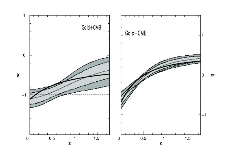
Figure 2: The comparison of results of $f(R)\propto R^{n}$ model with $n=1.296$ and $\beta=0.467$ (the thick solid line) to results of analysis of SNe+CMB data with $\Omega_{m}=0.29$ done in [5]. The evolution of the deceleration parameter with redshift is shown in a right panel and variation of equation of state of DE is shown in a left panel. The best fit of SNe+CMB data in such case is represented by the thin solid line, the $1\sigma$ and $2\sigma$ confidence levels are represented by the light and dark grey contours, respectively, and $\Lambda$CDM is represented by the dashed line.

As a set of observational data, the analysis of SNe and CMB data from [5] has been used. In that paper authors have reconstructed the resent history of the Universe on the base of SNe and CMB data in the model-independent way, only modeling DE by the hydrodynamical equation of state

$$p=w\rho,\quad w=(2q-1)/(3-\Omega_{m}/h^{2}).$$ (33)

The cited paper presents two conceptions of the analysis of the observational data: the first of them is the best fit to the data which uses only the hydrodynamical describing of DE and does not impose restrictions on the values of $\Omega_{m}$ and $h_{0}$, while the second conception follows the priority of the concordance $\Lambda$CDM model, so authors of [5] put $\Omega_{m}=0.27\pm 0.04$ and $h_{0}=0.71\pm 0.06$.

We will give the comparison of our results with both of them. Also we notice that the analogy of the “hydrodynamical” DE (33) is not so proper to the higher order gravity theories, hence one can expect the comparison over the values $h$ and $q$ to be more informative than over the value $w$.

As it has been found in [5], the best fit values are: $\Omega_{m}=0.385,h_{0}=60$. In the model DE evolves in time strongly enough. For given $\Omega_{m}$ and $h_{0}$ we compared the results of the $f(R)$-model with $n=1.2955\,(\delta n=0.0002)$ and $\beta=0.273$ for the “geometric equation of state” parameter $w=(y-ay^{\prime})/3(y-\Omega_{m}\,a)$ and the deceleration parameter $q$ with the results of [5]. In this $f(R)$-model the age of the Universe is $14.9$ Hyr, the deceleration parameter is $q_{0}=-0.91$ at present and the transition to acceleration occurs at $z=0.38$. Similarly to results of [5], the $w_{DE}<-1$ at lower redshifts ($w_{DE0}=-1.53$), however , the evolution of equation of state of “geometric DE” is more weak contrary to the results of [5].

However, if strong priors have been imposed on $\Omega_{m}$ and $h_{0}$ (i.e. the $\Lambda$CDM model priors: $\Omega_{m}=0.27\pm 0.04$ and $h_{0}=0.71\pm 0.06$), the evolution of DE is extremely weak and in good agreement with the $\Lambda$CDM model. The best fit in the case is $\Omega_{m}=0.29$ and there is a good enough coincidence of our model and their analysis for parameters of the model $n=1.296\,(\delta n=0.001)$ and $\beta=0.467$ (see Fig. 2). The deceleration parameter $q_{0}=-0.683$ at present, and the deceleration was changed by the acceleration at $z=0.51$ ($q_{0}=-0.63\pm 0.12$ and $z=0.57\pm 0.07$ in [5]). The age of the Universe in this case is 13.6 Hyr.

Thus, the $f(R)\propto\beta R^{n}$-model with parameters $\beta$ and $n$ chosen according to the principles mentioned in Introduction describes the evolution of the Universe quite corresponding to the SNe+CMB data.

References

- [1] A.Riess et al., Astron. J. 116, 1009 (1998); astro-ph/9805201.
- [2] S. J. Perlmutter et al., Astroph. J. 517, 565 (1999); arXiv:astro-ph/9812133.
- [3] M.Tegmark et al., Astroph. J. 606, 702 (2004); astro-ph/0310725.
- [4] J. Kratochvil, A. Linde, E.V.Linder, M.Shmakova, astro-ph/0312183.
- [5] U. Alam, V. Sahni, A. A. Starobinsky, JCAP 0406, 008 (2004); astro-ph/0403687.
- [6] A.G. Riess, et al., astro-ph/0402512.
- [7] J.D. Barrow, S. Cotsakis, Phys.Lett. B 214, 515 (1988).
- [8] M.B. Baibosunov, V.Ts. Gurovich, U.M. Imanaliev, Sov.Phys. JETP 71, 636 (1990).
- [9] V.Ts. Gurovich, Sov. DAN 195, 1300 (1970) (In Russian).
- [10] B.Ratra and P.J.E. Peebels, Phys. Rev. D 37, 3406 (1988).
- [11] I.Zlatev, L. Wang, P.J. Steinhardt, Phys. Rev. Lett. 82, 896 (1999).
- [12] V.Sahni and A.A.Starobinsky, IJMP D 9, 373 (2000).
- [13] A.Kamenshchik, U. Moschella, and V. Pasquier, Phys. Lett. B 511, 265 (2001).
- [14] S.M.Carroll, A. De Felice, V.Duvvuri, D. A. Easson, M.Trodden, M.S. Turner, Phys.Rev. D71, 063513 (2005).
- [15] S. Capozziello, V.F. Cardone, S. Carloni, A. Troisi, Int. J. Mod. Phys. D12, 1969 (2003).
- [16] V. Folomeev, V. Gurovich and H. Kleinert, astro-ph/0501209.
- [17] V.Ts. Gurovich and A. A. Starobinsky, Sov. Phys. JETP 50, 844 (1979).
- [18] A.A. Starobinsky, Phys. Lett. B 91, 99 (1980).
- [19] V. Gurovich and I. Tokareva, astro-ph/0509071.
- [20] S. M. Carroll, V. Duvvuri, M. Trodden and M. S. Turner, Phys. Rev. D 70, 043528 (2004).
- [21] T. Multamaki and I. Vilja, astro-ph/0506692.
- [22] V. Sahni, astro-ph/0403324; A.D. Dolgov, hep-ph/0405089.