Magnetic Field Spectrum at Cosmological Recombination

Abstract

A generation of magnetic fields from cosmological density perturbations is investigated. In the primordial plasma before cosmological recombination, all of the materials except dark matter in the universe exist in the form of photons, electrons, and protons (and a small number of light elements). Due to the different scattering nature of photons off electrons and protons, electric currents and electric fields are inevitably induced, and thus magnetic fields are generated. We present a detailed formalism of the generation of cosmological magnetic fields based on the framework of the well-established cosmological perturbation theory following our previous works. We numerically obtain the power spectrum of magnetic fields for a wide range of scales, from $k\sim 10^{-5}$ Mpc^-1 up to $k\sim 2\times 10^{4}$ Mpc^-1 and provide its analytic interpretation. Implications of these cosmologically generated magnetic fields are discussed.

I Introduction

There are observational evidences which indicate that magnetic fields exist not only galaxies, but also in even larger systems, such as cluster of galaxies and extra-cluster spaces Widrow (2002). In addition to gravity, they would play an important role in the formation processes of various objects and their dynamical evolution in the universe. The effects of large scale magnetic fields on galaxy formation and on formation of the first stars are extensively studied Gazzola et al. (2006); Dolag et al. (2001, 1999); Silk and Langer (2006); Machida et al. (2006).

Yet, the origin of such large scale magnetic fields is still a mystery Widrow (2002). It is now widely believed that the magnetic fields at large scales are amplified from a tiny field and maintained by the hydro-magnetic processes, i.e., the dynamo. However, the dynamo needs a seed field to act on and does not explain the origin of magnetic fields. As far as the magnetic fields in galaxies are concerned, the seed fields as large as $10^{-20\sim-30}$ G are required in order to account for the observed fields Davis et al. (1999) of order $1\mu$ G at the present universe. Discoveries of magnetic fields at damped Ly$\alpha$ systems Wolfe et al. (1992) in the early universe and an intervening galaxy at intermediate redshift Kronberg et al. (1992) may require even larger seed fields.

The question arises here is, thus, what is the origin of such seed fields? Most of previous theories to explain the origin of seed fields can be categorized into two, i.e., astrophysical and cosmological mechanisms. Almost all astrophysical mechanisms of generating seed magnetic fields are based on the Biermann battery effect Biermann and Schlüter (1951). This mechanism is operative when the gradients in thermodynamic quantities, such as temperature and density, are not parallel to that of pressure. This mechanism has been applied to various astrophysical systems, which include stars Kemp (1982), supernova remnants Miranda et al. (1998); Hanayama et al. (2005), protogalaxies Davies and Widrow (2000), large-scale structure formation Kulsrud et al. (1997), and ionization front at cosmological recombination Gnedin et al. (2000). These studies show that magnetic fields with amplitude $10^{-16}$ $\sim$ $10^{-21}$ G could be generated. Recently, it is proposed that the Weibel instability at the structure formation shocks can generate rather strong magnetic fields $10^{-7}$ G Fujita and Kato (2005); Medvedev et al. (2005). However, the coherence-length of seed fields generated by astrophysical mechanisms, especially the Weibel instability, tends to be too small to account for galaxy-scale magnetic fields.

On the other hand, cosmological mechanisms based on inflation can produce magnetic fields with a large coherence length since accelerating expansion during inflation can stretche small-scale fields to scales that can exceed the causal horizon. However, in the simplest models with the usual electromagnetic field, which is conformally coupled to gravity, the energy density in a fluctuation of the field diminishes as $a^{-4}$ (where $a$ is cosmic scale factor) to lead a negligible amplitude of magnetic fields at the end of inflation. Therefore, to create enough amount of magnetic fields which survive an expansion of the universe until today, some exotic couplings between the electromagnetic field to other fields, such as dilaton Ratra (1992); Bamba and Yokoyama (2004), Higgs type scalar particles Prokopec and Puchwein (2004), or gravity Turner and Widrow (1988), must be introduced. Although some models of them are considered to be natural extensions of standard particle model, the nature of generated magnetic fields depends highly on the way of extension, whose validity can never be tested experimentally by terrestrial particle accelerators. Moreover, it is recently argued that almost all models that generate magnetic fields during inflation at the galactic scale ($\lambda\sim 0.1$ Mpc) are severely constrained as $B_{\lambda}\mathrel{\mathchoice{\lower 3.6pt\vbox{\halign{$\mathsurround=0pt\displaystyle\hfil#\hfil$\cr<\crcr\sim\crcr}}}{\lower 3.6pt\vbox{\halign{$\mathsurround=0pt\textstyle\hfil#\hfil$\cr<\crcr\sim\crcr}}}{\lower 3.6pt\vbox{\halign{$\mathsurround=0pt\scriptstyle\hfil#\hfil$\cr<\crcr\sim\crcr}}}{\lower 3.6pt\vbox{\halign{$\mathsurround=0pt\scriptscriptstyle\hfil#\hfil$\cr<\crcr\sim\crcr}}}}10^{-39}$ G Caprini and Durrer (2002, 2005), for a blue primordial spectrum. This is because anisotropic stress of magnetic fields would produce a large amount of gravitational waves, which then spoil the standard Big Bang nucleosynthesis by bringing an overproduction of helium nuclei (and deuterium).

In addition to the two categories described above, however, there is a third category for the generation of large-scale seed fields: cosmological fluctuations in the universe can create magnetic fields prior to cosmological recombination. This category dates back to Harrison (1970) Harrison (1970) and has been rigorously studied in recent years. The attractive point is that mechanisms based on cosmological perturbations are much less ambiguous than the previous two categories because cosmological pertrubations have now been well understood both theoretically and observationally through cosmic microwave background (CMB) anisotropy and large scale structure of the universe. Thus it is possible to make a robust quantitative evaluation of the generated magnetic fields.

Originally, Harrison found that the vorticity in a primordial plasma can generate magnetic fields. This is because electrons and ions would tend to spin at different rates as the universe expands due to the radiation drag on electrons, arising rotation-type electric current and thus inducing magnetic fields. It was found that magnetic fields of $10^{-21}$ G would result if the vorticity is equivalent to galactic rotation by $z=10$. More recently, magnetic field generation at recombination was investigated by evaluating the induced electric field which arise in the matter flow dragged by a dipole photon field, resulting in a seed field $10^{-26}$ G Hogan (2000). Following Harrison’s idea, Matarrese reported that $10^{-29}$ G seed fields can arise from the vorticity generated by second-order density perturbations at recombination Matarrese et al. (2005). In a similar analysis, a larger value, $10^{-21}$ G, was obtained by considering earlier periods when the energy density of photons was larger and the photon mean free path was smaller Berezhiani and Dolgov (2004). Other specific second order effects from the coupling between density and velocity fluctuations on the seed field generation was evaluated in Gopal and Sethi (2005).

In Takahashi et al. (2005), we presented a formalism to calculate the spectrum of seed fields based on the cosmological perturbation theory. There are three essential points in order to obtain the correct spectrum. First of all, we have to treat electron, proton and photon fluids separately to evaluate the amount of electric current and electric field. Secondly, we need a precise evaluation of collision terms between three fluids, which generate the difference in motion between them. At this point, we found that not only the velocity difference between electron and photon fluids, which is conventionally studied, but also photon anisotropic stress contributes to the difference in motion between electron and proton fluids. Finally, the second-order perturbation theory is necessary because vector-type perturbations, such as vorticity and magnetic field, are known to be absent at the first order. Based on this formalism, in Ichiki et al. (2006), we calculated the spectrum of generated magnetic fields at a range between $k\sim 10^{-5}$ Mpc^-1 and $k\sim 10$ Mpc^-1. Then we showed that the magnetic field is contributed mainly from the velocity difference between electrons and photons, which we called the ”baryon-photon slip term”, on large scales ($k\lesssim 1$ Mpc^-1), while photon anisotropic stress is dominant on small scalles ($k\gtrsim 1$ Mpc^-1). As a whole, the spectrum is small-scale-dominant and the amplitude is about $10^{-20}$ G at $k=1$ Mpc^-1.

In this paper, we present details of our formalism and extend it in several directions. First, in section II, we describe the derivation of equations of motion for electron and proton fluids, carefully evaluating the collision term between electrons and photons, and then obtain the evolution equation for magnetic fields. We calculate and interpret the resulting spectrum numerically in section III. In section IV, we derive the analytical expression of the spectrum, which allows us to confirm the numerical results and extrapolate the spectrum into much smaller scales than can be obtained numerically. In section V, we discuss about the magnetic felicity, which in fact explicitly vanishes. Finally, in section VI, we give some discussions and conclusions.

II Basic Equations

Here we derive basic equations for the generation of magnetic fields, i.e., perturbation equations of photon, proton and electron fluids. While protons and electrons are conventionally treated as a single fluid, however, it is necessary to deal with proton and electron fluids separately in order to discuss the generation of magnetic fields. Let us begin with the Euler equations. Those are given by

$$m_{p}nu_{p}^{\mu}u_{pi;\mu}-enu_{p}^{\mu}F_{i\mu}=C^{pe}_{~{}i}+C^{p\gamma}_{~{}i},$$ (1)

$$m_{e}nu_{e}^{\mu}u_{ei;\mu}+enu_{e}^{\mu}F_{i\mu}=C^{ep}_{~{}i}+C^{e\gamma}_{~{}i}~{},$$ (2)

where $m_{p(e)}$ is the proton (electron) mass, $u_{p(e)}$ is the bulk velocity of protons (electrons), $F_{\mu i}$ is the usual Maxwell tensor. The thermal pressure of proton and electron fluids are neglected. Here $\mu,\nu=0,1,2,3$ and $i=1,2,3$. The r.h.s. of Eq. (1) and (2) represent the collision terms. The first terms in Eqs. (1) and (2) are collision terms for the Coulomb scattering between protons and electrons, which is given by

$$C^{pe}_{i}=-C^{ep}_{i}=-(u_{pi}-u_{ei})e^{2}n^{2}\eta~{},$$ (3)

where

$$\eta=\frac{\pi e^{2}m_{e}^{1/2}}{(k_{B}T_{e})^{3/2}}\ln\Lambda\sim 9.4\times 10^{-16}{\rm sec}\left(\frac{1+z}{10^{5}}\right)^{-3/2}\left(\frac{\ln\Lambda}{10}\right)~{},$$ (4)

is the resistivity of the plasma and $\ln\Lambda$ is the Coulomb logarithm. As is well known, this term acts as the diffusion term in the evolution equation of magnetic field. The importance of the diffusion effect can be estimated by the diffusion scale,

$$\lambda_{\rm diff}\equiv\sqrt{\eta\tau}\sim 100\left(\frac{\tau}{H_{0}^{-1}}\right)^{1/2}{\rm AU},$$ (5)

above which magnetic field cannot diffuse in the time-scale $\tau$. Here $H_{0}=70{\rm km/s/Mpc}$ is the present Hubble parameter. Thus, at cosmological scales considered in this paper, this term can be safely neglected.

The other terms expressed by $C^{p(e)\gamma}_{~{}i}$ are the collision terms for Compton scattering of protons (electrons) with photons. Since photons scatter off electrons preferentially compared with protons by a factor of $(m_{e}/m_{p})^{2}$, we can safely drop the term $C^{p\gamma}_{~{}i}$ from the Euler equation of protons. This difference in collision terms between protons and electrons ensures that small difference in velocity between protons and electrons, that is, electric current, is indeed generated once the Compton scattering becomes effective.

II.1 Compton Collision Term

Let us now evaluate the Compton scattering term. In the limit of completely elastic collisions between photons and electrons, this term vanishes. Typically, in the regime of interest in this paper, very little energy is transfered between electrons and photons in Compton scatterings. Therefore it is a good approximation to expand the collision term systematically in powers of the energy transfer.

Let us demonstrate this specifically. We consider the collision process

$$\gamma(p_{i})+e^{-}(q_{i})\rightarrow\gamma(p^{\prime}_{i})+e^{-}(q^{\prime}_{i}),$$ (6)

where the quantities in the parentheses denote the particle momenta. To calculate this process, we evaluate the collision term in the Boltzmann equation of photons:

$$C[f(\vec{p})] = \frac{a}{p}\int\frac{d^{3}q}{(2\pi)^{3}2E_{e}(q)}\int\frac{d^{3}q^{\prime}}{(2\pi)^{3}2E_{e}(q^{\prime})}\int\frac{d^{3}p^{\prime}}{(2\pi)^{3}2E(p^{\prime})}(2\pi)^{4}|M|^{2}$$ (7)

$$\times\delta^{(3)}[\vec{p}+\vec{q}-\vec{p^{\prime}}-\vec{q^{\prime}}]\delta[E(p)+E_{e}(q)-E(p^{\prime})-E_{e}(q^{\prime})]$$

$$\times[f_{e}(\vec{q^{\prime}})f(\vec{p^{\prime}})(1+f(\vec{p}))-f_{e}(\vec{q})f(\vec{p})(1+f(\vec{p^{\prime}}))]~{},$$

where $f(\vec{p})$ and $f_{e}(\vec{q})$ are the distribution functions of photons and electrons, $E_{e}(q)=\sqrt{q^{2}+m_{e}^{2}}$ is the energy of an electron, and the delta functions enforce the energy and momentum conservations. We have dropped the Pauli blocking factor $(1-f_{e})$. The Pauli blocking factor can be always omitted safely in the epoch of interest, because $f_{e}$ is very small after electron-positron annihilations. Note that the stimulating factor can be also dropped because this does not contribute to the Euler equation.

Integrating over $\vec{q^{\prime}}$, we obtain

$$C[f(\vec{p})] = \frac{a}{p}\int\frac{d^{3}q}{(2\pi)^{3}2E_{e}(q)}\int\frac{d^{3}p^{\prime}}{(2\pi)^{3}2E(p^{\prime})}\frac{(2\pi)}{2E_{e}(|\vec{q}+\vec{p}-\vec{p^{\prime}}|)}|M|^{2}$$ (8)

$$\times\delta[E(p)+E_{e}(q)-E(p^{\prime})-E_{e}(|\vec{q}+\vec{p}-\vec{p^{\prime}}|)]$$

$$\times[f_{e}(\vec{q}+\vec{p}-\vec{p^{\prime}})f(\vec{p^{\prime}})-f_{e}(\vec{q})f(\vec{p})]~{}.$$

In the regime of our interest, energy transfer through the Compton scattering is small and can be ignored in the first order density perturbations. As we already discussed earlier, however, it is essential to take the second order couplings in the Compton scattering term into consideration for generation of magnetic fields. Therefore we expand the collision term up to the first order in powers of the energy transfer^†, and keep terms up to second order in density perturbations.

The expansion parameter is the energy transfer,

$$E_{e}(q)-E_{e}(q^{\prime})=\frac{q^{2}}{2m_{e}}-\frac{(\vec{q}+\vec{p}-\vec{p^{\prime}})^{2}}{2m_{e}}\approx\frac{(\vec{p^{\prime}}-\vec{p})\cdot\vec{q}}{m_{e}}-\frac{(\vec{p}-\vec{p^{\prime}})^{2}}{2m_{e}}~{},$$ (9)

over the temperature of the universe. Employing $p\sim T$, we can estimate the order of this expansion parameter as ${\cal O}(\frac{pq}{m_{e}T})\sim{\cal O}(\frac{q}{m_{e}})$, which is small when electrons are non-relativistic. Note that, in the cosmological Thomson regime, electrons in the thermal bath of photons are non-relativistic, $p\sim\frac{q^{2}}{2m_{e}}$, and the energy of photons is much smaller than the rest mass of a electron, $p\ll m_{e}$. Thus, it also holds that $q\sim\sqrt{2m_{e}p}\gg p$, and the second term in Eq.(9) is usually smaller than the first one.

Now let us divide the collision integral into four parts, i.e., the denominators of the Lorentz volume, the scattering amplitude, the delta function and the distribution functions, and expand them due to the expansion parameter defined above. First of all, the denominator in the Lorentz invariant volume can be expanded to

$$\frac{1}{E_{e}(q)E_{e}(|\vec{q}+\vec{p}-\vec{p^{\prime}}|)} = \left(m_{e}+\frac{1}{2m_{e}}|\vec{q}+\vec{p}-\vec{p^{\prime}}|^{2}\right)^{-1}\left(m_{e}+\frac{1}{2m_{e}}|\vec{q}|^{2}\right)^{-1}$$ (10)

$$\approx \frac{1}{m_{e}^{2}}\left(1-{\cal E}_{(\frac{q}{m_{e}})^{2}}-{\cal E}_{(\frac{pq}{m_{e}^{2}})}-{\cal E}_{(\frac{p}{m_{e}})^{2}}\right),$$

where

$${\cal E}_{(\frac{q}{m_{e}})^{2}}=\frac{q^{2}}{m_{e}^{2}},~{}~{}~{}{\cal E}_{(\frac{qp}{m_{e}^{2}})}=\frac{(\vec{p}-\vec{p^{\prime}})\cdot\vec{q}}{m_{e}^{2}},~{}~{}~{}{\cal E}_{(\frac{p}{m_{e}})^{2}}=\frac{(\vec{p}-\vec{p^{\prime}})^{2}}{2m_{e}^{2}}.$$ (11)

Secondly, we consider the matrix element. The matrix element for Compton scattering in the rest frame of the electron is given by,

$$|M|^{2} = 2(4\pi)^{2}\alpha^{2}\left[\frac{\tilde{p^{\prime}}}{\tilde{p}}+\frac{\tilde{p}}{\tilde{p^{\prime}}}-\sin^{2}\tilde{\beta}\right]~{},$$

$$\cos\tilde{\beta} = \tilde{\hat{p}}\cdot\tilde{\hat{p}}^{\prime}~{},$$ (12)

where $\tilde{p}$ and $\tilde{p^{\prime}}$ are the energies of incident and scattered photons, $\tilde{\hat{p}}$ and $\tilde{\hat{p}}^{\prime}$ are the unit vectors of $\tilde{\vec{p}}$ and $\tilde{\vec{p}}^{\prime}$, respectively, denoting the directions of the photons in this frame. The Lorentz transformation with electron’s velocity ($q/m_{e}$) gives the following relations,

$$\frac{p}{\tilde{p}} = \frac{\sqrt{1-(q/m_{e})^{2}}}{1-\vec{p}\cdot{\vec{q}}/pm_{e}},$$ (13)

$$p_{\mu}p^{\mu} = \tilde{p_{\mu}}\tilde{p^{\mu}}.$$ (14)

Using these relations, we evaluate the matrix element in the CMB frame as Hu (1995)

$$|M|^{2} = 2(4\pi)^{2}\alpha^{2}\left({\cal M}_{0}+{\cal M}_{\frac{q}{m_{e}}}+{\cal M}_{(\frac{q}{m_{e}})^{2}}+{\cal M}_{(\frac{qp}{m_{e}^{2}})}+{\cal M}_{(\frac{p}{m_{e}})^{2}}\right)~{},$$ (15)

$${\cal M}_{0} = 1+\cos^{2}\beta~{},$$ (16)

$${\cal M}_{\frac{q}{m_{e}}} = -2\cos\beta(1-\cos\beta)\left[\frac{\vec{q}}{m_{e}}\cdot\left(\hat{p}+\hat{p^{\prime}}\right)\right]~{},$$ (17)

$${\cal M}_{(\frac{q}{m_{e}})^{2}} = 2\cos\beta(1-\cos\beta)\frac{q^{2}}{m_{e}^{2}}~{},$$ (18)

$${\cal M}_{\frac{qp}{m_{e}^{2}}} = (1-\cos\beta)(1-3\cos\beta)\left[\frac{\vec{q}}{m_{e}}\cdot(\hat{p}+\hat{p^{\prime}})\right]^{2}+2\cos\beta(1-\cos\beta)\frac{(\vec{q}\cdot\hat{p})(\vec{q}\cdot\hat{p^{\prime}})}{m_{e}^{2}}~{},$$ (19)

$${\cal M}_{(\frac{p}{m_{e}})^{2}} = (1-\cos\beta)^{2}\frac{p^{2}}{m_{e}^{2}}~{}.$$ (20)

Thirdly, we expand the delta function to

$$\delta[p-p^{\prime}+E_{e}(q)-E_{e}(q^{\prime})]$$

$$\approx\delta(p-p^{\prime})-\frac{\partial\delta(p-p^{\prime}+E_{e}(q)-E_{e}(q^{\prime}))}{\partial E_{e}(q^{\prime})}|_{E_{e}(q)=E_{e}(q^{\prime})}\left(E_{e}(q)-E_{e}(q^{\prime})\right)$$

$$~{}~{}~{}+\frac{1}{2}\frac{\partial^{2}\delta(p-p^{\prime}+E_{e}(q)-E_{e}(q^{\prime}))}{\partial p^{2}}|_{E_{e}(q)=E_{e}(q^{\prime})}\left(E_{e}(q)-E_{e}(q^{\prime})\right)^{2}$$

$$=\delta(p-p^{\prime})+\frac{\partial\delta(p-p^{\prime})}{\partial p^{\prime}}\left[\frac{(\vec{p}-\vec{p^{\prime}})\cdot\vec{q}}{m_{e}}+\frac{(p-p^{\prime})^{2}}{2m_{e}}\right]+\frac{1}{2}\left[\frac{(\vec{p}-\vec{p^{\prime}})\cdot\vec{q}}{m_{e}}\right]^{2}\frac{\partial^{2}\delta(p-p^{\prime})}{\partial{p^{\prime}}^{2}}$$

$$\equiv\delta(p-p^{\prime})+\frac{\partial\delta(p-p^{\prime})}{\partial p^{\prime}}\left[{\cal D}_{(\frac{q}{m})}+{\cal D}_{(\frac{p}{m})}\right]+\frac{1}{2}{\cal D}^{2}_{(\frac{q}{m})}\frac{\partial^{2}\delta(p-p^{\prime})}{\partial{p^{\prime}}^{2}}.$$ (21)

where

$${\cal D}_{(\frac{q}{m})}\equiv\frac{(\vec{p}-\vec{p^{\prime}})\cdot\vec{q}}{m_{e}},~{}~{}~{}{\cal D}_{(\frac{p}{m})}\equiv\frac{(p-p^{\prime})^{2}}{2m_{e}}.$$ (22)

Finally, the distribution of the electron can be expanded to

$$f_{e}(\vec{q}+\vec{p}-\vec{p^{\prime}})\approx f_{e}(\vec{q})+\frac{\partial f_{e}}{\partial\vec{q}}\cdot(\vec{p}-\vec{p^{\prime}})+(p^{i}-{p^{\prime}}^{i})\frac{\partial^{2}f_{e}}{\partial q^{i}\partial q^{j}}(p^{j}-{p^{\prime}}^{j}).$$ (23)

We assume that the electrons are kept in thermal equilibrium and in the Boltzmann distribution:

$$f_{e}(\vec{q})=n_{e}\left(\frac{2\pi}{m_{e}T_{e}}\right)^{3/2}\exp\left[-\frac{(\vec{q}-m_{e}\vec{v_{e}})^{2}}{2m_{e}T_{e}}\right]~{},$$ (24)

where $v_{e}$ is the bulk velocity of electrons. The derivatives of the distribution function with respect to the momentum are given as

$$\frac{\partial f_{e}}{\partial\vec{q}} = -f_{e}(\vec{q})\frac{\vec{q}-m_{e}\vec{v_{e}}}{m_{e}T_{e}}~{},$$ (25)

$$\frac{\partial^{2}f_{e}}{\partial q_{i}\partial q_{j}} = -\frac{\partial f_{e}(\vec{q})}{\partial q_{j}}\frac{q^{i}-m_{e}v^{i}}{m_{e}T_{e}}-f_{e}(\vec{q})\frac{\delta_{ij}}{m_{e}T_{e}}~{}.$$ (26)

By substituting above equations, Eq.(23) is written as

$$f_{e}(\vec{q}+\vec{p}-\vec{p^{\prime}}) \approx f_{e}(\vec{q})-f_{e}(\vec{q})\frac{\vec{q}-m_{e}\vec{v_{e}}}{m_{e}T_{e}}\cdot(\vec{p}-\vec{p^{\prime}})+\frac{1}{2}f_{e}(\vec{q})\left[\left[\frac{(\vec{p}-\vec{p^{\prime}})(\vec{q}-m_{e}\vec{v_{e}})}{m_{e}T_{e}}\right]^{2}-\frac{|\vec{p}-\vec{p^{\prime}}|^{2}}{m_{e}T_{e}}\right]$$ (27)

$$\equiv f_{e}(\vec{q})\left[1-{\cal F}_{(\frac{q}{m})}+\frac{1}{2}{\cal F}_{(\frac{q}{m})}^{2}-{\cal F}_{(\frac{p}{m})}\right]~{}.$$

Therefore, we have

$$f_{e}(\vec{q}+\vec{p}-\vec{p^{\prime}})f(\vec{p^{\prime}})-f_{e}(\vec{q})f(\vec{p})=f_{e}(\vec{q})\left[f(\vec{p^{\prime}})-f(\vec{p})\right]-f(\vec{p^{\prime}})f_{e}(\vec{q}){\cal F}_{(\frac{q}{m})}-f(\vec{p^{\prime}})f_{e}(\vec{q})\left[{\cal F}_{(\frac{T}{m})}-\frac{1}{2}{\cal F}^{2}_{(\frac{q}{m})}\right]~{}.$$ (28)

Fortunately, it has been known that the leading term (zeroth order term), obtained by multiplying together the first term in the delta function and the zeroth order distribution functions, is zero. It means that we only have to keep up to the first order terms when we expand the matrix element and the energies, in order to keep the collision term up to the second order Dodelson and Jubas (1995).

Therefore we have,

$$\frac{|M|^{2}}{E_{e}(q)E_{e}(q^{\prime})}\approx 6\pi\sigma_{T}({\cal M}_{0}+{\cal M}_{\frac{q}{m_{e}}})$$ (29)

Combining altogether, we obtain the collision term expanded with respect to the energy transfer as (note that this expansion is not with respect to the density perturbations)

$$C[f]=\frac{a}{p}\left(\frac{\pi}{4}\right)\int\frac{d^{3}p^{\prime}}{(2\pi)^{3}p^{\prime}}\frac{d^{3}q}{(2\pi)^{3}}\left[{\mbox{(0th order term)}}+{\mbox{(1st order terms)}}+{\mbox{(2nd order terms)}}\right]+\cdot\cdot\cdot$$ (30)

where

0th order term: (31)

$$6\pi\sigma_{T}{\cal M}_{0}\delta(p-p^{\prime})f_{e}(\vec{q})\left[f(\vec{p^{\prime}})-f(\vec{p}))\right],$$

1st order terms: (32)

$$6\pi\sigma_{T}{\cal M}_{0}f_{e}(\vec{q})\left[-\delta(p-p^{\prime})f(\vec{p^{\prime}}){\cal F}_{\frac{q}{m}}+\frac{\partial\delta(p-p^{\prime})}{\partial p^{\prime}}{\cal D}_{\frac{q}{m}}\left[f(\vec{p^{\prime}})-f(\vec{p})\right]\right]$$

$$+6\pi\sigma_{T}{\cal M}_{\frac{q}{m}}f_{e}(\vec{q})\delta(p-p^{\prime})\left[f(\vec{p^{\prime}})-f(\vec{p})\right],$$

2nd order terms: (33)

$$6\pi\sigma_{T}{\cal M}_{0}f_{e}(\vec{q})\Biggl{[}-\delta(p-p^{\prime})f(\vec{p^{\prime}})\left[{\cal F}_{\frac{p}{m}}-\frac{1}{2}{\cal F}^{2}_{\frac{q}{m}}\right]+\frac{1}{2}\frac{\partial^{2}\delta(p-p^{\prime})}{\partial{p^{\prime}}^{2}}{\cal D}^{2}_{\frac{q}{m}}\left[f(\vec{p^{\prime}})-f(\vec{p})\right]$$

$$+\frac{\partial\delta(p-p^{\prime})}{\partial p^{\prime}}{\cal D}_{\frac{p}{m}}\left[f(\vec{p^{\prime}})-f(\vec{p})\right]-\frac{\partial\delta(p-p^{\prime})}{\partial p^{\prime}}\left({\cal D}_{\frac{q}{m}}+{\cal D}_{\frac{p}{m}}\right)f(\vec{p^{\prime}}){\cal F}_{\frac{q}{m}}\Biggr{]}$$

$$+6\pi\sigma_{T}{\cal M}_{\frac{q}{m}}f_{e}(\vec{q})\left[-\delta(p-p^{\prime})f(\vec{p^{\prime}}){\cal F}_{\frac{q}{m}}+\frac{\partial\delta(p-p^{\prime})}{\partial p^{\prime}}\left({\cal D}_{\frac{q}{m}}+{\cal D}_{\frac{p}{m}}\left[f(\vec{p^{\prime}}-f(\vec{p}))\right]\right)\right].$$

From now on, we omit the second order terms. These terms are not only much smaller than the first order terms but also may not contribute to the Euler equation at all (see Bartolo et al. (2006)). Evaluating the first moment of the above collision term, we obtain the Compton scattering term in the Euler equation (41) as

$$C^{e\gamma}_{i} = -\int\frac{d^{3}p}{(2\pi)^{3}}p_{i}C[f]$$ (34)

$$= -\frac{4\sigma_{T}\rho_{\gamma}an_{e}}{3}\left[(v_{ei}-v_{\gamma i})+\frac{1}{4}v_{ej}\Pi^{\phantom{\gamma}j}_{\gamma i}\right].$$

Here moments of the distribution functions are given by

$$\int\frac{d^{3}p}{(2\pi)^{3}}pf_{\gamma}(\vec{p})=\rho_{\gamma},$$ (35)

$$\int\frac{d^{3}p}{(2\pi)^{3}}p_{i}f_{\gamma}(\vec{p})=\frac{4}{3}\rho_{\gamma}v_{\gamma i},$$ (36)

$$\int\frac{d^{3}q}{(2\pi)^{3}}f_{e}(\vec{q})=n_{e},$$ (37)

$$\int\frac{d^{3}q}{(2\pi)^{3}}q_{i}f_{e}(\vec{q})=\rho_{e}v_{ei},$$ (38)

$$\int\frac{d^{3}p}{(2\pi)^{3}}p^{-1}p_{i}p_{j}f_{\gamma}(\vec{p})=\frac{1}{3}\rho_{\gamma}\Pi_{\gamma ij}+\frac{1}{3}\rho_{\gamma}\delta_{ij},$$ (39)

where $\rho_{\gamma}$ and $\rho_{e}(=m_{e}n_{e})$ are energy densities of photons and electrons, $v^{i}_{\gamma}$ and $v^{i}_{e}$ are their bulk three velocities defined by $v^{i}\equiv u^{i}/u^{0}$, and $\Pi^{ij}_{\gamma}$ is anisotropic stress of photons. It should be noted that the collision term (34) was obtained nonperturbatively with respect to density perturbations Takahashi et al. (2005).

II.2 Evolution Equations of Magnetic Fields

Now we obtain the Euler equations for protons and electrons as

$$m_{p}nu_{p}^{\mu}u_{pi;\mu}-enu_{p}^{\mu}F_{i\mu}=0,$$ (40)

$$m_{e}nu_{e}^{\mu}u_{ei;\mu}+enu_{e}^{\mu}F_{i\mu}=-\frac{4\sigma_{T}\rho_{\gamma}an}{3}\left[(v_{ei}-v_{\gamma i})+\frac{1}{4}v_{ej}\Pi_{\gamma i}^{\phantom{\gamma}j}\right],$$ (41)

where $m_{p}$ is the proton mass. Here we ignore the pressure of proton and electron fluids. Also the Coulomb collision term is neglected as explained below Eq. (5). Note that the collision term was not evaluated in a manifestly covariant way. Here the left hand side in Eqs. (40) and (41) should be evaluated in conformal coordinate system. We also assumed the local charge neutrality: $n=n_{e}\sim n_{p}$. In the case without electromagnetic fields ($F_{i\mu}=0$), the sum of the equations (40) and (41) gives the Euler equation for the baryons in the standard perturbation theory. On the other hand, subtracting Eq. (40) multiplied by $m_{e}$ from Eq. (41) multiplied by $m_{p}$, we obtain

$$-\frac{m_{p}m_{e}}{e}\left[nu^{\mu}\left(\frac{j_{i}}{n}\right)_{;\mu}+j^{\mu}\left(\frac{m_{p}-m_{e}}{m_{p}+m_{e}}\frac{j_{i}}{en}-u_{i}\right)_{;\mu}\right]+en(m_{p}+m_{e})u^{\mu}F_{i\mu}-(m_{p}-m_{e})j^{\mu}F_{i\mu}$$

$$=-\frac{4m_{p}\rho_{\gamma}an\sigma_{T}}{3}\left[(v_{ei}-v_{\gamma i})+\frac{1}{4}v_{ej}\Pi_{\gamma i}^{\phantom{\gamma}j}\right],$$ (42)

where $u^{\mu}$ and $j^{\mu}$ are the center-of-mass 4-velocity of the proton and electron fluids and the net electric current, respectively, defined as

$$u^{\mu}\equiv\frac{m_{p}u_{p}^{\mu}+m_{e}u_{e}^{\mu}}{m_{p}+m_{e}},$$ (43)

$$j^{\mu}\equiv en(u_{p}^{\mu}-u_{e}^{\mu}).$$ (44)

Employing the Maxwell equations $F^{\mu\nu}_{;\nu}=j^{\mu}$, we see that the quantities in the square bracket in the l.h.s. of Eq. (42) is suppressed at the recombination epoch, compared to the second term, by a factor Subramanian et al. (1994)

$$\frac{c^{2}}{L^{2}\omega_{p}^{2}}\sim 3\times 10^{-40}\left(\frac{10^{3}{\rm cm}^{-3}}{n}\right)\left(\frac{1{\rm Mpc}}{L}\right)^{2},$$ (45)

where $c$ is the speed of light, $L$ is a characteristic length of the system and $\omega_{p}=\sqrt{4\pi ne^{2}/m_{e}}$ is the plasma frequency.

The third term in the l.h.s. of Eq. (42), i.e., $(m_{p}-m_{e})j^{\mu}F_{i\mu}$, is the Hall term which can also be neglected because the Coulomb coupling between protons and electrons is so tight that $|u^{i}|\gg|u_{p}^{i}-u_{e}^{i}|$. Then we obtain a generalized Ohm’s law:

$$u^{\mu}F_{i\mu}=-\frac{4\sigma_{T}\rho_{\gamma}a}{3e}\left[(v_{ei}-v_{\gamma i})+\frac{1}{4}v_{ej}\Pi_{\gamma i}^{\phantom{\gamma}j}\right]\equiv C_{i}.$$ (46)

Now we derive the evolution equation for the magnetic field, which can be obtained from the Bianchi identities $F_{[\mu\nu,\lambda]}=0$, as

$$0 = \frac{3}{2}\epsilon^{ijk}u^{\mu}F_{[jk,\mu]}$$ (47)

$$= u^{\mu}{\cal B}^{i}_{~{},\mu}-\epsilon^{ijk}\left(C_{j,k}+\frac{u^{0}_{~{},j}}{u^{0}}C_{k}\right)-(u^{i}_{~{},j}{\cal B}^{j}-u^{j}_{~{},j}{\cal B}^{i})+\frac{u^{0}_{~{},j}}{u^{0}}({\cal B}^{j}u^{i}-{\cal B}^{i}u^{j}),$$

where $\epsilon^{ijk}$ is the Levi-Cività tensor and ${\cal B}^{i}\equiv(a^{2}B^{i})=\epsilon^{ijk}F_{jk}/2$ is the magnetic field in the comoving frame Jedamzik et al. (1998). We will now expand the photon energy density, fluid velocities and photon anisotropic stress with respect to the density perturbation as

$$\rho_{\gamma}(t,x_{i})=\stackrel{{\scriptstyle\mbox{\tiny(0)}}}{{\rho}}_{\gamma}(t)+\stackrel{{\scriptstyle\mbox{\tiny(1)}}}{{\rho}}_{\gamma}(t,x_{i})+\cdots,~{}~{}~{}u^{0}(t,x_{i})=a(t)^{-1}+\stackrel{{\scriptstyle\mbox{\tiny(1)}}}{{u}}^{0}(t,x_{i})+\cdots,$$

$$u^{i}(t,x_{i})=\stackrel{{\scriptstyle\mbox{\tiny(1)}}}{{u}}^{i}(t,x_{i})+\stackrel{{\scriptstyle\mbox{\tiny(2)}}}{{u}}^{i}(t,x_{i})+\cdots,~{}~{}~{}v_{i}(t,x_{i})=\stackrel{{\scriptstyle\mbox{\tiny(1)}}}{{v}}_{i}(t,x_{i})+\stackrel{{\scriptstyle\mbox{\tiny(2)}}}{{v}}_{i}(t,x_{i})+\cdots$$

$$\Pi_{\gamma}^{ij}(t,x_{i})=\stackrel{{\scriptstyle\mbox{\tiny(1)}}}{{\Pi}}_{\gamma}^{ij}(t,x_{i})+\cdots,$$ (48)

where the superscripts $(0),(1)$, and $(2)$ denote the order of expansion and $t$ is the cosmic time. Remembering that ${\cal B}^{i}$ is a second-order quantity, we see that all terms involving ${\cal B}^{i}$ in Eq. (47), other than the first term, can be neglected. Thus we obtain

$$\frac{d{\cal B}^{i}}{dt} \sim \epsilon^{ijk}\left(C_{j,k}+\frac{u^{0}_{~{},j}}{u^{0}}C_{k}\right)$$ (49)

$$= \frac{4\sigma_{T}\stackrel{{\scriptstyle\mbox{\tiny(0)}}}{{\rho}}_{\gamma}a}{3e}\epsilon^{ijk}\Biggl{[}\left(\stackrel{{\scriptstyle\mbox{\tiny(1)}}}{{\delta_{\gamma,j}}}-2\stackrel{{\scriptstyle\mbox{\tiny(1)}}}{{\Phi}}_{,j}\right)\left(\stackrel{{\scriptstyle\mbox{\tiny(1)}}}{{v}}_{ek}-\stackrel{{\scriptstyle\mbox{\tiny(1)}}}{{v}}_{\gamma k}\right)-\frac{1}{4}\left(\stackrel{{\scriptstyle\mbox{\tiny(1)}}}{{v}}_{el}\stackrel{{\scriptstyle\mbox{\tiny(1)}}}{{\Pi}}{}^{l}_{\gamma j}\right)_{,k}-2\stackrel{{\scriptstyle\mbox{\tiny(1)}}}{{h}}^{l}_{~{}j,k}\left(\stackrel{{\scriptstyle\mbox{\tiny(1)}}}{{v}}_{el}-\stackrel{{\scriptstyle\mbox{\tiny(1)}}}{{v}}_{\gamma l}\right)-\left(\stackrel{{\scriptstyle\mbox{\tiny(2)}}}{{v}}_{ej,k}-\stackrel{{\scriptstyle\mbox{\tiny(2)}}}{{v}}_{\gamma j,k}\right)\Biggr{]},$$

where $\stackrel{{\scriptstyle\mbox{\tiny(1)}}}{{\Phi}}$ and $\stackrel{{\scriptstyle\mbox{\tiny(1)}}}{{h}}^{i}_{~{}j}$ are first-order curvature and tensor perturbations, respectively, in Poisson gauge, and we used the density contrast of photons, $\stackrel{{\scriptstyle\mbox{\tiny(1)}}}{{\delta}}_{\gamma,k}\equiv\stackrel{{\scriptstyle\mbox{\tiny(1)}}}{{\rho}}_{\gamma,k}/\stackrel{{\scriptstyle\mbox{\tiny(0)}}}{{\rho}}_{\gamma}$. Further, we employed the fact that there is no vorticity in the linear order: $\epsilon^{ijk}\stackrel{{\scriptstyle\mbox{\tiny(1)}}}{{v}}_{j,k}=0$. It should be noted that the velocity of electron fluid can be approximated to the center-of-mass velocity at this order, $\stackrel{{\scriptstyle\mbox{\tiny(1)}}}{{v}}_{e}^{i}\sim\stackrel{{\scriptstyle\mbox{\tiny(1)}}}{{v}}^{i}$. The physical meaning of this equation is that electrons gain (or lose) their momentum through scatterings due to the relative velocity to photons (baryon-photon slip), and the anisotropic pressure from photons. The momentum transfer from the photons ensures the velocity difference between electrons and protons, and thus eventually generates magnetic fields. We found that the contribution from the curvature perturbation is always much smaller than that from the density contrast of photons in the first term in Eq.(49) (which will be clearly seen in Figs.1 and 2). Therefore we shall omit the curvature perturbation hereafter when considering the evolution of magnetic fields.

The first term in Eq. (49) is exactly the same discussed in Gopal and Sethi (2005). They have estimated contributions from these terms by considering typical values at recombination. Here we solve the equation numerically and obtain a robust prediction of the amplitude of magnetic fields.

Eq.(49) shows that the magnetic field cannot be generated in the first (linear) order. The r.h.s. of Eq.(49) contains two kinds of source terms, i.e., intrinsic second order quantities and products of first order quantities. Since the first order quantities can be exactly evaluated within the frame work of the standard cosmological linear perturbation theory, we hereafter concentrate on the products of first order quantities. The evaluation of the intrinsic second order term will be left for the future work.

III Cosmological Magnetic Fields

III.1 Spectrum of Cosmologically Generated Magnetic Fields

In this section we derive the spectrum of magnetic fields generated by cosmological perturbations. The cosmological perturbations can be decomposed into scalar, vector, and tensor modes. These modes physically correspond to perturbations of density, vorticity and gravitational waves, respectively. These cosmological perturbations are most likely to be generated during the inflation epoch. Most of the simple single field inflation models predict generation of adiabatic scalar and tensor type perturbations but vector type perturbations. Even if the vector type perturbations are generated, they are known to be damped away in the expanding universe. Observations of CMB temperature fluctuations and large scale structure of the universe strongly suggest the adiabatic scalar perturbations while we only have upper limits on tensor perturbations Seljak et al. (2005). Therefore at most tensor perturbations are only sub-dominant components. Hence we consider only scalar type perturbations for linear order quantities throughout this paper.

The linear-order scalar perturbations can be written as

$$\delta_{\gamma,k} = \frac{1}{\sqrt{(2\pi)^{3}}}\int(ik_{k})\delta_{\gamma}(\vec{k},t)e^{i\vec{k}\cdot\vec{x}}d^{3}\vec{k},$$ (50)

$$v_{el} = \frac{1}{\sqrt{(2\pi)^{3}}}\int(-i\hat{k}_{l})v_{e}(\vec{k},t)e^{i\vec{k}\cdot\vec{x}}d^{3}\vec{k},$$ (51)

$$v_{el,k} = \frac{1}{\sqrt{(2\pi)^{3}}}\int\hat{k}_{l}k_{k}v_{e}(\vec{k},t)e^{i\vec{k}\cdot\vec{x}}d^{3}\vec{k},$$ (52)

$$\Pi^{l}_{j} = \frac{1}{\sqrt{(2\pi)^{3}}}\int(-\hat{k}^{l}\hat{k}_{j}+\frac{1}{3}\delta^{l}_{j})\Pi(\vec{k},t)e^{i\vec{k}\cdot\vec{x}}d^{3}\vec{k},$$ (53)

$$\Pi^{l}_{j,k} = \frac{1}{\sqrt{(2\pi)^{3}}}\int(ik_{k})(-\hat{k}^{l}\hat{k}_{j}+\frac{1}{3}\delta^{l}_{j})\Pi(\vec{k},t)e^{i\vec{k}\cdot\vec{x}}d^{3}\vec{k}.$$ (54)

Here $\hat{k}^{i}\equiv k^{i}/k$. By using these expressions, we can write the evolution equation of magnetic fields in Fourier space as,

$$(a^{2}{B^{i}}(\vec{K},t))^{\cdot}=\frac{4\sigma_{T}\rho_{\gamma}}{3e}\epsilon^{ijk}\frac{1}{\sqrt{(2\pi)^{3}}}\int d^{3}\vec{k^{\prime}}\left[\hat{k}^{\prime}_{j}K_{k}\delta_{\gamma}(\vec{K}-\vec{k^{\prime}},t)\delta v(\vec{k^{\prime}},t)-\frac{1}{4}\alpha_{jk}(\vec{K},\vec{k^{\prime}})v_{e}(\vec{K}-\vec{k^{\prime}},t)\Pi(\vec{k^{\prime}},t)\right]$$ (55)

where we have defined,

$$\delta v = v_{e}-v_{\gamma},$$ (56)

$$\alpha_{jk}(\vec{K},\vec{k^{\prime}}) = \frac{K}{|\vec{K}-\vec{k^{\prime}}|}\left(K(\hat{K}\cdot\hat{k}^{\prime})-\frac{4}{3}k^{\prime}\right)\hat{K}_{k}\hat{k}_{j}^{\prime}.$$ (57)

To obtain the spectrum, one needs to evaluate $\left<B^{i}(\vec{K})B^{\ast}_{i}(\vec{K^{\prime}})\right>=S(K)\delta(\vec{K}-\vec{K^{\prime}})$. That is

$$a^{4}B^{i}(\vec{K})B^{*}_{i}(\vec{K^{\prime}}) = \left(\frac{4\sigma_{T}}{3e}\right)^{2}\epsilon^{ijk}\epsilon^{lm}_{i}\displaystyle\frac{1}{(2\pi)^{3}}\int d^{3}\vec{k^{\prime}}d^{3}\vec{k}\int_{0}^{t_{0}}dt^{\prime}\int_{0}^{t_{0}}dt^{\prime\prime}$$ (58)

$$\times \biggl{[}\hat{k}^{\prime}_{j}K_{k}\delta_{\gamma}(\vec{K}-\vec{k^{\prime}},t^{\prime})\delta v(\vec{k^{\prime}},t^{\prime})a(t^{\prime})\rho_{\gamma}(t^{\prime})\hat{k}_{l}K^{\prime}_{m}\delta^{*}_{\gamma}(\vec{K^{\prime}}-\vec{k},t^{\prime\prime})\delta v^{*}(\vec{k},t^{\prime\prime})a(t^{\prime\prime})\rho_{\gamma}(t^{\prime\prime})$$

$$-\frac{1}{4}\hat{k}^{\prime}_{j}K_{k}\delta_{\gamma}(\vec{K}-\vec{k^{\prime}},t^{\prime})\delta v(\vec{k^{\prime}},t^{\prime})a(t^{\prime})\rho_{\gamma}(t^{\prime})\alpha_{lm}(\vec{K^{\prime}},\vec{k})v^{*}_{e}(\vec{K^{\prime}}-\vec{k},t^{\prime\prime})\Pi^{*}(\vec{k},t^{\prime\prime})a(t^{\prime\prime})\rho_{\gamma}(t^{\prime\prime})$$

$$-\frac{1}{4}\alpha_{lm}(\vec{K},\vec{k^{\prime}})v_{e}(\vec{K}-\vec{k^{\prime}},t^{\prime})\Pi(\vec{k^{\prime}},t^{\prime})a(t^{\prime})\rho_{\gamma}(t^{\prime})\hat{k}_{l}K^{\prime}_{m}\delta^{*}_{\gamma}(\vec{K^{\prime}}-\vec{k},t^{\prime\prime})\delta v^{*}(\vec{k},t^{\prime\prime})a(t^{\prime\prime})\rho_{\gamma}(t^{\prime\prime})$$

$$+\frac{1}{16}\alpha_{jk}(\vec{K},\vec{k^{\prime}})v_{e}(\vec{K}-\vec{k^{\prime}},t^{\prime})\Pi(\vec{k^{\prime}},t^{\prime})a(t^{\prime})\rho_{\gamma}(t^{\prime})\alpha_{lm}(\vec{K^{\prime}},\vec{k})v_{e}^{*}(\vec{K^{\prime}}-\vec{k},t^{\prime\prime})\Pi^{*}(\vec{k},t^{\prime\prime})a(t^{\prime\prime})\rho_{\gamma}(t^{\prime\prime})\biggl{]}~{}.$$

The final task we should do is to take an ensemble average of this expression. Assuming that perturbations are random Gaussian variables and using the Wick’s theorem, we can expand the ensemble average of the products of four Gaussian variables as, for example,

$$\left<\delta_{\gamma}(\vec{K}-\vec{k^{\prime}},t^{\prime})\delta v(\vec{k^{\prime}},t^{\prime})\delta_{\gamma}^{*}(\vec{K^{\prime}}-\vec{k},t^{\prime\prime})\delta v^{*}(\vec{k},t^{\prime\prime})\right> = \left<\delta_{\gamma}(\vec{K}-\vec{k^{\prime}},t^{\prime})\delta v(\vec{k^{\prime}},t^{\prime})\right>\left<\delta_{\gamma}^{*}(\vec{K^{\prime}}-\vec{k},t^{\prime\prime})\delta v^{*}(\vec{k},t^{\prime\prime})\right>$$

$$+ \left<\delta_{\gamma}(\vec{K}-\vec{k^{\prime}},t^{\prime})\delta_{\gamma}^{*}(\vec{K^{\prime}}-\vec{k},t^{\prime\prime})\right>\left<\delta v(\vec{k^{\prime}},t^{\prime})\delta v^{*}(\vec{k},t^{\prime\prime})\right>$$

$$+ \left<\delta_{\gamma}(\vec{K}-\vec{k^{\prime}},t^{\prime})\delta v^{*}(\vec{k},t^{\prime\prime})\right>\left<\delta v(\vec{k^{\prime}},t^{\prime})\delta_{\gamma}^{*}(\vec{K^{\prime}}-\vec{k},t^{\prime\prime})\right>~{}.$$

Since the evolution equations for linear order perturbation variables are independent of $\hat{k}$, we may write

$$\delta_{\gamma}(\vec{k},t) = \psi_{i}(\vec{k})\delta_{\gamma}(k,t)~{},$$ (60)

$$\delta v(\vec{k},t) = \psi_{i}(\vec{k})\delta v(k,t)~{},$$ (61)

$$\Pi(\vec{k},t) = \psi_{i}(\vec{k})\Pi(k,t)~{},$$ (62)

where $\psi_{i}(\vec{k})$ is the initial perturbation and $\delta_{\gamma}(k,t),\delta u(k,t)$, and $\Pi(k,t)$ are the transfer functions, which are the solution of the Einstein-Boltzmann equations under the adiabatic initial condition with $\psi_{i}(\vec{k})=1$. By virtue of linearized equations, the overall amplitude and spectrum of the primordial fluctuations, $P(k)$, can be given independently of the transfer functions. Here $P(k)$ is defined using the two-point correlation function of $\psi_{i}$ in Fourier space,

$$\left<\psi_{i}(\vec{k})\psi_{i}^{*}(\vec{k^{\prime}})\right>=P(k)\delta(\vec{k}-\vec{k^{\prime}})~{},$$ (63)

where $\delta$ is the Dirac delta function. According to the convention, we write $P(k)\propto k^{n_{s}-4}$ with $n_{s}$ being the spectral index of primordial density perturbations. Using these definitions, we finally obtain,

$$S(K) = \left(\frac{4\sigma_{T}}{3e}\right)^{2}\int\frac{d^{3}\vec{k}}{(2\pi)^{3}}K^{2}\left[1-(\hat{k}\cdot\hat{K})^{2}\right]P(|\vec{K}-\vec{k}|)P(k)$$ (64)

$$\times\biggl{\{}S_{1}^{2}(|\vec{K}-\vec{k}|,k)-\frac{k}{|\vec{K}-\vec{k}|}S_{1}(k,|\vec{K}-\vec{k}|)S_{1}(|\vec{K}-\vec{k}|,k)$$

$$~{}~{}~{}+\frac{1}{4}\left[\beta S_{2}(k,|\vec{K}-\vec{k}|)S_{1}(|\vec{K}-\vec{k}|,k)-\frac{k}{|\vec{K}-\vec{k}|}\alpha S_{1}(k,|\vec{K}-\vec{k}|)S_{2}(|\vec{K}-\vec{k}|,k)\right]$$

$$~{}~{}~{}+\frac{1}{16}\alpha\left[\alpha S_{2}^{2}(|\vec{K}-\vec{k}|,k)-\beta S_{2}(k,|\vec{K}-\vec{k}|)S_{2}(|\vec{K}-\vec{k}|,k)\right]\biggr{\}}~{},$$

where

$$S_{1}(k,k^{\prime}) = \int a(t^{\prime})\rho_{\gamma}(t^{\prime})\delta_{\gamma}(k,t^{\prime})\delta v(k^{\prime},t^{\prime})dt^{\prime}~{},$$ (65)

$$S_{2}(k,k^{\prime}) = \int a(t^{\prime})\rho_{\gamma}(t^{\prime})v_{e}(k,t^{\prime})\Pi_{\gamma}(k^{\prime},t^{\prime})dt^{\prime}~{},$$ (66)

$$\alpha = \frac{3K(\hat{K}\cdot\hat{k})-2k}{3|\vec{K}-\vec{k}|}~{},$$ (67)

$$\beta = \frac{K\left\{K-k(\hat{K}\cdot\hat{k})\right\}}{|\vec{K}-\vec{k}|^{2}}-\frac{2}{3}~{}.$$ (68)

Here $S_{1}$ and $S_{2}$ describe effects of baryon-photon slip and photon anisotropic pressure. Specifically, the terms in the second and fourth lines in Eq.(64) are what we will call in subsequent sections the contributions to the generation of magnetic fields from baryon-photon slip and anisotropic stress of photons, respectively.

III.2 Cosmological Perturbation Theory and Numerical Calculations

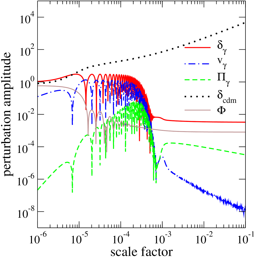
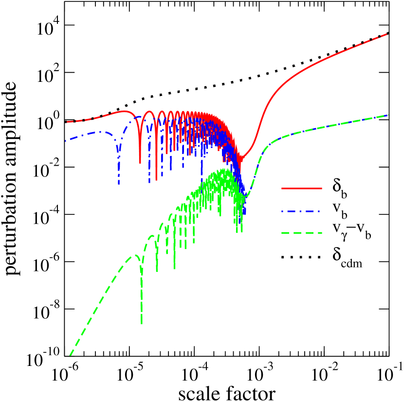
Figure 1: Evolution of perturbations relevant with magnetic field generation in a $\Lambda$CDM model with wavenumber $k/h=1.6$ Mpc^-1. Left: the five lines represent density contrast of CDM ($\delta_{\rm CDM}$; black dotted line), and density contrast ($\delta_{\gamma}$; red line) , velocity perturbation ($v_{\gamma}$; blue dash-dotted line), anisotropic stress ($\Pi_{\gamma}$; green dashed line) of photons, and curvature perturbation ($\Phi$; brown thin line) as indicated. Right: time evolutions of density contrast ($\delta_{b}$; red line) and velocity perturbation ($v_{b}$; blue dash-dotted line) of baryons. The baryon-photon slip ($v_{\gamma}-v_{e}$; blue dash-dotted line) is also shown in the figure. In the deep radiation dominated era, baryon-photon slip and anisotropic stress of photons are severely suppressed compared to the other perturbation variables. Perturbation variables are shown in the Newtonian gauge Ma and Bertschinger (1995) while anisotropic stress and slip terms are gauge invariant.

Evolutions of perturbations relevant to the generation of magnetic fields can be solved within the frame work of the standard cosmological perturbation theory. The standard theory describing evolutions of linear perturbations, which was originally developed by Lifshiz Lifshitz (1946) and summarized in his textbook Landau and Lifshitz (1971) and other recent articles Kodama and Sasaki (1984); Mukhanov et al. (1992), is well tested by a number of observations and firmly established. As for an application to cosmological models, the first realistic numerical calculation was done by Peebles & Yu Peebles and Yu (1970), where the distribution of photons was solved by directory integrating the Boltzmann equation. The calculations were subsequently extended to include neutrinos Bond and Szalay (1983), and non-baryonic dark matter Bond and Efstathiou (1984). These calculations, especially the resulting angular spectrum of CMB photons, are fully understood within an analytic treatment by Hu & Sugiyama Hu and Sugiyama (1995).

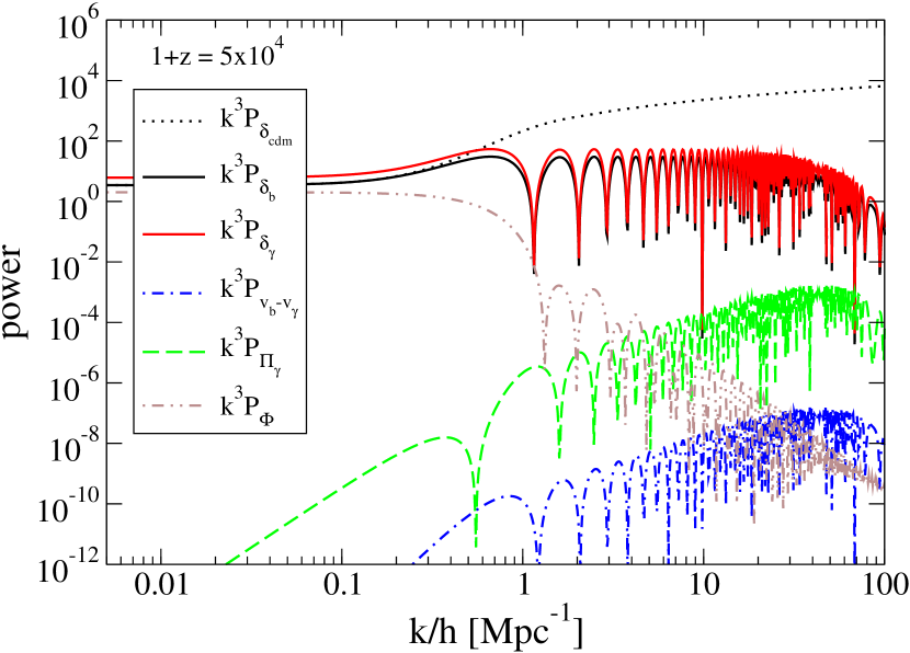
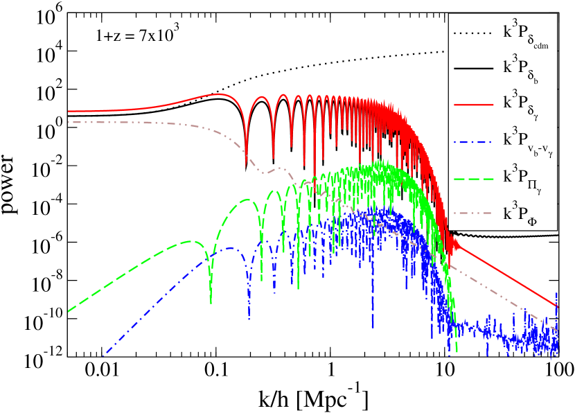
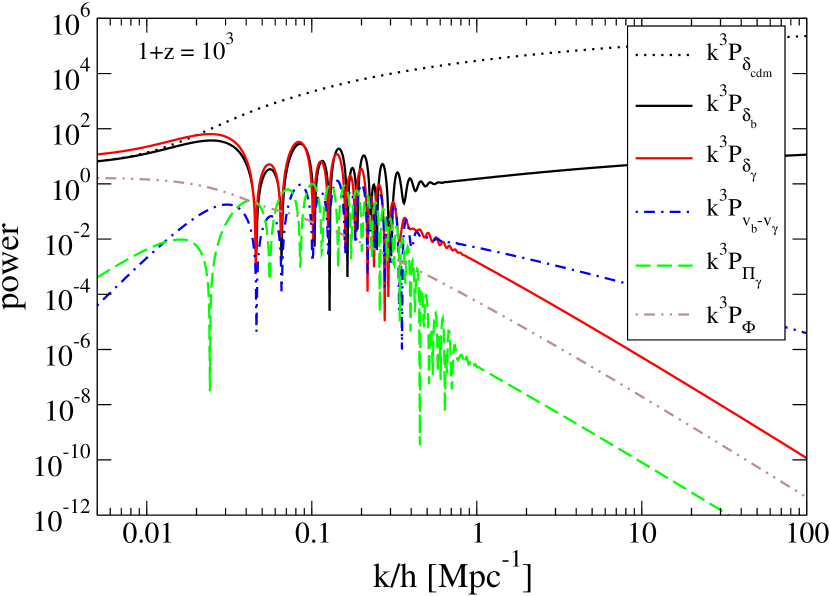
Figure 2: Spectra of $\delta_{\rm CDM}$ (black dotted line), $\delta_{b}$ (thick black line), $\delta_{\gamma}$ (thin red line), $\Pi_{\gamma}$ (green dashed line), $v_{b}-v_{\gamma}$ (blue dash-dotted line), and $\Phi$ (brown dash-dot-dotted line) at redshift $z=10^{3}$ (bottom left), $7\times 10^{3}$ (top right), $5\times 10^{4}$ (top left). In general, the spectra at each redshift are divided into four parts from large scales to small ones: primordial spectra at super-horizon scales, acoustic oscillation spectra at sub-horizon scales, exponentially damping spectra at diffusion scales, and power law phase after the diffusion damping. In acoustic oscillation scales at each redshift, the amplitudes of density perturbations of baryons ($\delta_{b}$) and photons ($\delta_{\gamma}$) stay constant, while baryon-photon slip ($v_{e}-v_{\gamma}$) and anisotropic stress of photons ($\Pi_{\gamma}$) show larger power at relatively smaller scales. Powers in baryon-photon slip and anisotropic stress of photons get larger at lower redshift.

Evolutions of the linear quantities such as $\delta$, $v$, and $\Pi$ in an expanding universe can now be easily solved by the publicly available Einstein-Boltzmann code such as CMBFAST Seljak and Zaldarriaga (1996) or CAMB Lewis et al. (2000). In Fig. 1, we show an example of the evolution of perturbations with wavenumber $k/h=1.6$ Mpc^-1 in standard $\Lambda$CDM cosmology. Time evolutions can be typically divided into four characteristic eras. First, the modes of perturbations are beyond the cosmic horizon (era I; $a\mathrel{\mathchoice{\lower 3.6pt\vbox{\halign{$\mathsurround=0pt\displaystyle\hfil#\hfil$\cr<\crcr\sim\crcr}}}{\lower 3.6pt\vbox{\halign{$\mathsurround=0pt\textstyle\hfil#\hfil$\cr<\crcr\sim\crcr}}}{\lower 3.6pt\vbox{\halign{$\mathsurround=0pt\scriptstyle\hfil#\hfil$\cr<\crcr\sim\crcr}}}{\lower 3.6pt\vbox{\halign{$\mathsurround=0pt\scriptscriptstyle\hfil#\hfil$\cr<\crcr\sim\crcr}}}}10^{-5}$ in Fig. 1). After the horizon crossing, the baryon-photon fluid undergoes acoustic oscillations (era II; $10^{-5}\mathrel{\mathchoice{\lower 3.6pt\vbox{\halign{$\mathsurround=0pt\displaystyle\hfil#\hfil$\cr<\crcr\sim\crcr}}}{\lower 3.6pt\vbox{\halign{$\mathsurround=0pt\textstyle\hfil#\hfil$\cr<\crcr\sim\crcr}}}{\lower 3.6pt\vbox{\halign{$\mathsurround=0pt\scriptstyle\hfil#\hfil$\cr<\crcr\sim\crcr}}}{\lower 3.6pt\vbox{\halign{$\mathsurround=0pt\scriptscriptstyle\hfil#\hfil$\cr<\crcr\sim\crcr}}}}a\mathrel{\mathchoice{\lower 3.6pt\vbox{\halign{$\mathsurround=0pt\displaystyle\hfil#\hfil$\cr<\crcr\sim\crcr}}}{\lower 3.6pt\vbox{\halign{$\mathsurround=0pt\textstyle\hfil#\hfil$\cr<\crcr\sim\crcr}}}{\lower 3.6pt\vbox{\halign{$\mathsurround=0pt\scriptstyle\hfil#\hfil$\cr<\crcr\sim\crcr}}}{\lower 3.6pt\vbox{\halign{$\mathsurround=0pt\scriptscriptstyle\hfil#\hfil$\cr<\crcr\sim\crcr}}}}10^{-3.5}$) until the diffusion of photons erases the perturbations (era III; $10^{-3.5}\mathrel{\mathchoice{\lower 3.6pt\vbox{\halign{$\mathsurround=0pt\displaystyle\hfil#\hfil$\cr<\crcr\sim\crcr}}}{\lower 3.6pt\vbox{\halign{$\mathsurround=0pt\textstyle\hfil#\hfil$\cr<\crcr\sim\crcr}}}{\lower 3.6pt\vbox{\halign{$\mathsurround=0pt\scriptstyle\hfil#\hfil$\cr<\crcr\sim\crcr}}}{\lower 3.6pt\vbox{\halign{$\mathsurround=0pt\scriptscriptstyle\hfil#\hfil$\cr<\crcr\sim\crcr}}}}a\mathrel{\mathchoice{\lower 3.6pt\vbox{\halign{$\mathsurround=0pt\displaystyle\hfil#\hfil$\cr<\crcr\sim\crcr}}}{\lower 3.6pt\vbox{\halign{$\mathsurround=0pt\textstyle\hfil#\hfil$\cr<\crcr\sim\crcr}}}{\lower 3.6pt\vbox{\halign{$\mathsurround=0pt\scriptstyle\hfil#\hfil$\cr<\crcr\sim\crcr}}}{\lower 3.6pt\vbox{\halign{$\mathsurround=0pt\scriptscriptstyle\hfil#\hfil$\cr<\crcr\sim\crcr}}}}10^{-3}$) as the universe expands, while density perturbations of CDM grow mildly by their own gravity. After recombination (era IV; $a\mathrel{\mathchoice{\lower 3.6pt\vbox{\halign{$\mathsurround=0pt\displaystyle\hfil#\hfil$\cr>\crcr\sim\crcr}}}{\lower 3.6pt\vbox{\halign{$\mathsurround=0pt\textstyle\hfil#\hfil$\cr>\crcr\sim\crcr}}}{\lower 3.6pt\vbox{\halign{$\mathsurround=0pt\scriptstyle\hfil#\hfil$\cr>\crcr\sim\crcr}}}{\lower 3.6pt\vbox{\halign{$\mathsurround=0pt\scriptscriptstyle\hfil#\hfil$\cr>\crcr\sim\crcr}}}}10^{-3}$), photons and baryons are decoupled each other. In that era photons stream freely and baryons can evolve according to the gravitational potential of CDM.

All modes of perturbations in baryons and photons whose wave number is larger than $\sim 0.1$ Mpc^-1 are destined to be erased before recombination by Silk damping Silk (1968). Therefore, each perturbation mode with such wavenumber can contribute to the generation of magnetic fields only when the mode undergoes acoustic oscillations. During that era, density and velocity perturbations of baryons and photons show an oscillatory behavior and their amplitudes remain almost constant. Meanwhile the variables suppressed by tight coupling between photons and electrons, such as $v_{e}-v_{\gamma}$ or $\Pi_{\gamma}$, grow as the universe expands and the number density of electrons becomes smaller (see Fig. 1). Thus the spectra of perturbations have a peak at the scale of acoustic oscillations or the scale slightly larger than the diffusion scale at each epoch, that is clearly shown in Fig. 2.

We plot $\left(a\rho_{\gamma}/H\right)k^{3}P(k)\delta v(k)\delta_{\gamma}(k)$ and $\left(a\rho_{\gamma}/H\right)k^{3}P(k)v_{b}(k)\Pi_{\gamma}(k)$ in the left and right panels of Fig. 3. These spectra naively correspond to the source terms $S_{1}$ and $S_{2}$ in Eq. (64). Of course, the magnetic field spectrum should be obtained by a non-linear convolution of these spectra given by Eq. (64). However, because the smaller scale modes than the diffusion scale are absent at each redshift and thus the non-linear couplings mainly come from the modes with comparable wavenumbers, one can expect that the cosmologically generated magnetic fields will roughly have a spectrum similar to the envelope curves of these spectra.

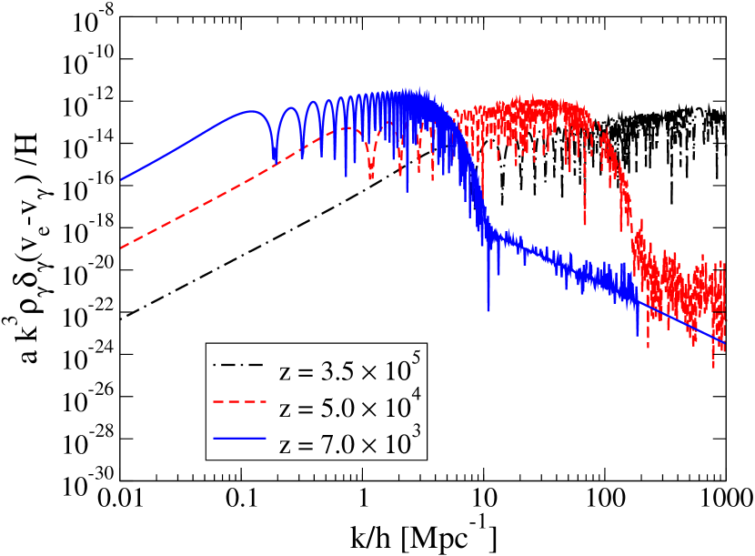
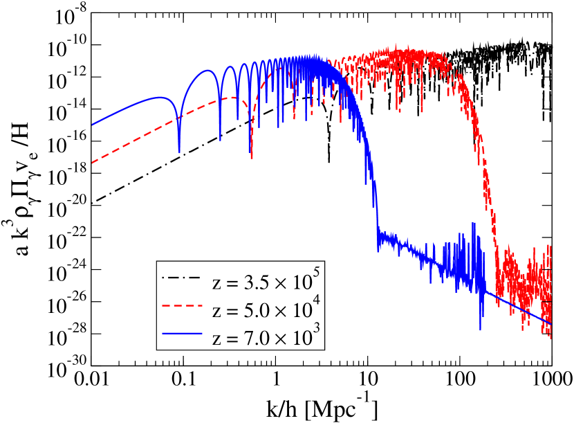
Figure 3: Plots of integrand per d$\log(1+z)$, $k^{3}\frac{\rho_{\gamma}}{H}\delta_{\gamma}(u_{e}-u_{\gamma})$ (left) and $k^{3}\frac{\rho_{\gamma}}{H}\Pi_{\gamma}u_{e}$ (right). The magnetic field spectrum results from non-linear convolution and time integration of these spectra. The contributions mainly comes from the waves between the scales of cosmic horizon, and the Silk diffusion at each redshift.

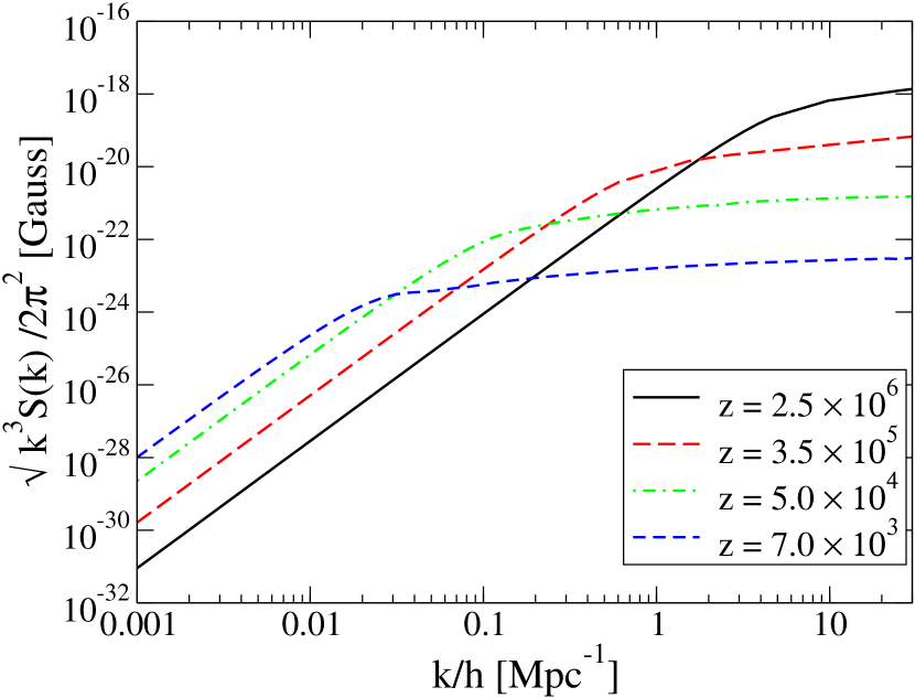
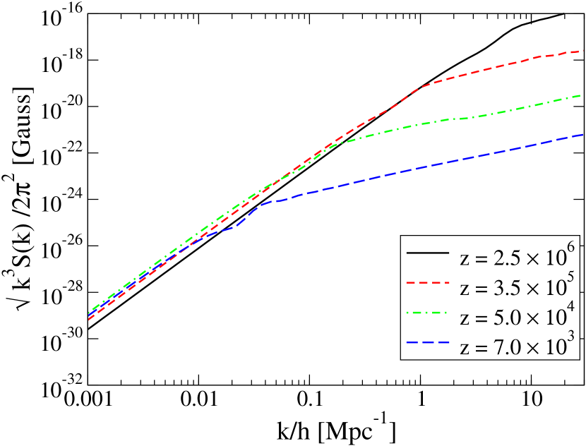
Figure 4: Time evolution of Spectra of conformal magnetic fields generated from baryon-photon slip (left) and anisotropic stress of photons (right). Corresponding redshifts are also indicated in the figures. For both contributions, the smaller scale fields are created at the higher redshift.

We numerically integrated Eq.(64) to obtain the magnetic field spectra. The cosmological parameters in our calculation are fixed to the standard $\Lambda$ CDM values in a flat universe, i.e.,

$$(h,n_{s},\Omega_{b},\Omega_{\Lambda},A)=(0.7,~{}1.0,~{}0.04,~{}0.70,~{}2.7\times 10^{-9})~{},$$ (69)

where $h$ is the current Hubble parameter in units of $100$km/s/Mpc, $n_{s}$ is the power spectrum index of primordial density fluctuations, $\Omega_{b}$ and $\Omega_{\Lambda}$ are energy densities in baryon and cosmological constant in units of the critical density, and $A$ is overall amplitude of density perturbation squared. Magnetic field spectra induced by baryon-photon slip and anisotropic stress of photons at different redshifts, which correspond to second and fourth lines of Eq.(64), respectively, are shown in left and right panels of Fig. 4. In these figures we take the combination of $\sqrt{k^{3}\left<BB^{*}\right>}/2\pi^{2}$ to show in units of Gauss. The spectra consist of two slopes. At super-horizon scales the slope is proportional to $k^{3.5}$ for both contributions while it becomes less steep at sub-horizon scales. The turning points of the spectra roughly correspond to the Hubble horizon scale at each redshift while it may be difficult to see clear turnoff in the spectra generated from anisotropic stress (right panel). Clearly, one can find that small scale magnetic fields are created at higher redshifts. After their generation, magnetic fields $B$ are adiabatically diminishing as $a^{-2}$. To see this fact more explicitly, we depict the time evolution of magnetic field with fixed wavenumber $K$ in Fig. 5. Analytic interpretation for these magnetic field spectra is given in the next section.

IV Analytic Interpretation of the Magnetic Field Spectrum

IV.1 Magnetic Field Spectrum at Large Scales

Magnetic fields are mainly created after the modes of perturbations with the corresponding scale enter the cosmic horizon and are causally contacted. Magnetic fields at larger scales than the cosmic horizon are generated only as a consequence of non-linear couplings of each Fourier mode. In the previous studies it was suggested that at largest scales the magnetic field spectrum generated from density perturbations has the power proportional to $k^{2}$ Matarrese et al. (2005). If one carefully evaluates, however, the terms proportional to $k^{2}$ exactly cancel each other out, and the spectrum starts from the term proportional to $k^{4}$ as we shall show below. In order to see this, let us consider the spectrum generated by the first term (baryon-photon slip term) in equation (49),

$$\left<B^{i}(\vec{K},t)B_{i}^{*}(\vec{K^{\prime}},t)\right> \propto \int d^{3}\vec{k}K^{2}\left\{1-(\hat{k}\cdot\hat{K})^{2}\right\}P(|\vec{K}-\vec{k}|)P(k)$$ (70)

$$\times\biggl{\{}S_{1}^{2}(|\vec{K}-\vec{k}|,k)-\frac{k}{|\vec{K}-\vec{k}|}S_{1}(k,|\vec{K}-\vec{k}|)S_{1}(|\vec{K}-\vec{k}|,k)\biggr{\}}~{}.$$

In the limit $K/k\to 0$, we can write

$$|\vec{K}-\vec{k}| = \sqrt{k^{2}-2kK\gamma+K^{2}}\approx k-K\gamma~{},$$

$$|\vec{K}-\vec{k}|^{-1} \approx k^{-1}\left(1+\frac{K}{k}\gamma\right)~{},$$

where $\gamma\equiv\hat{k}\cdot\hat{K}$. Furthermore, time integration terms can be treated as $K$ independent in the same limit, i.e., $S_{1}(|\vec{K}-\vec{k}|,k)\approx S_{1}(k,|\vec{K}-\vec{k}|)\approx T(k)$. Remembering that the spectrum of density perturbations is written as $P(k)\propto k^{n_{s}-4}$, we can rewrite equation (70) as

$$\left<B^{i}(\vec{K},t)B_{i}^{*}(\vec{K^{\prime}},t)\right> \propto \int k^{2}dk\int^{1}_{-1}d\gamma(1-\gamma^{2})P(|\vec{K}-\vec{k}|)P(k)K^{2}\left(1-\frac{k}{|\vec{K}-\vec{k}|}\right)T^{2}(k)$$ (71)

$$\approx \int k^{2}dk\int^{1}_{-1}d\gamma(\gamma-\gamma^{3})\left[k-(n_{s}-4)K\gamma\right]k^{n_{s}-4}\left(-\frac{K^{3}}{k}\right)T^{2}(k)$$

$$\propto K^{4}~{}.$$

We can see this non-linear power law tail at large scales in Fig. 4.

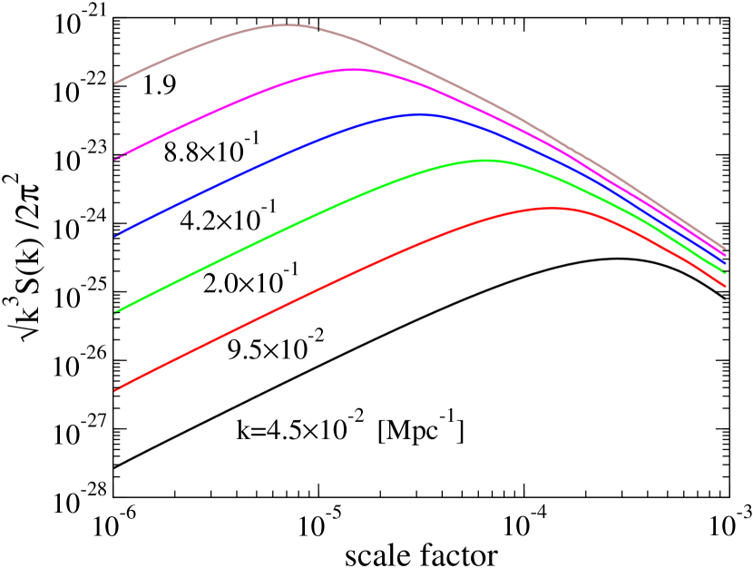
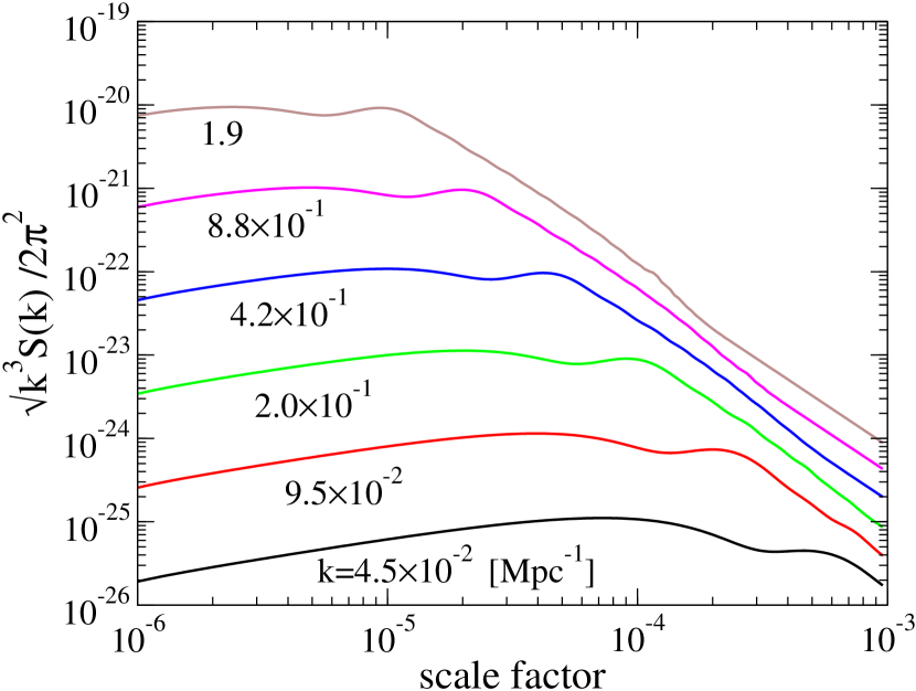
Figure 5: Time evolution of magnetic fields in units of Gauss, $\sqrt{k^{3}S(k)/2\pi^{2}}$, generated from baryon-photon slip (left) and anisotropic stress of photons (right) with fixed wavenumbers as indicated. Magnetic fields at smaller scales have been created earlier and their amplitudes are larger. After their generation magnetic fields diminish as $a^{-2}$ adiabatically.

IV.2 Magnetic Field Spectrum at Sub-horizon Scales

In this subsection we show that the behavior of the magnetic field spectrum at small scales can be understood within the standard theory of cosmological perturbations. Since Compton scattering is an essential process for generation of magnetic fields, magnetic fields start to be generated when the relevant modes come across the horizon and are causally connected. On the other hand, once the modes become shorter than the diffusion scale of photons, magnetic fields cannot be no longer generated. Therefore magnetic fields with wavenumber $K$ are mainly created from density perturbations with wavenumber $k\sim K\mathrel{\mathchoice{\lower 3.6pt\vbox{\halign{$\mathsurround=0pt\displaystyle\hfil#\hfil$\cr<\crcr\sim\crcr}}}{\lower 3.6pt\vbox{\halign{$\mathsurround=0pt\textstyle\hfil#\hfil$\cr<\crcr\sim\crcr}}}{\lower 3.6pt\vbox{\halign{$\mathsurround=0pt\scriptstyle\hfil#\hfil$\cr<\crcr\sim\crcr}}}{\lower 3.6pt\vbox{\halign{$\mathsurround=0pt\scriptscriptstyle\hfil#\hfil$\cr<\crcr\sim\crcr}}}}k_{\rm diff}$, where $k_{\rm diff}$ is the corresponding wavenumber of the diffusion scale at each time. Within the approximation that $k\sim K$, $|\vec{K}-\vec{k}|\sim K$, the spectrum of magnetic fields is roughly given by

$$S(k)\sim\left(\frac{4\sigma_{T}}{3e}\right)^{2}\left(\int d^{3}kk^{2}s_{1}^{2}+\int d^{3}kk^{2}s_{2}^{2}\right)~{},$$ (72)

where

$$s_{1} \equiv P(k)S_{1}(k,k)~{},$$ (73)

$$s_{2} \equiv P(k)S_{2}(k,k)~{}.$$ (74)

Here we neglected sub-dominant cross correlating terms. We have already plotted $k^{3}s_{1}\propto k^{3}\frac{a\rho_{\gamma}}{H}P(k)\delta v(k)\delta_{\gamma}$ and $k^{3}s_{2}\propto k^{3}\frac{a\rho_{\gamma}}{H}P(k)v_{b}(k)\Pi_{\gamma}$ in the left and right panels of Fig. 3. These spectra indeed indicate that magnetic fields are created when the modes of perturbations come across the cosmic horizon and undergo acoustic oscillations. In fact, the largest contributions come from the modes of perturbations slightly larger than the diffusion scale.

The behavior of acoustic oscillations in the early universe can be analytically understood by using tight coupling approximations. In the tight coupling regime, Compton scattering occurs sufficient enough so that photons and baryons (electrons) can behave as a coupled fluid. Therefore, the baryon-photon slip ($v_{b}-v_{\gamma}$) and the anisotropic stress of photons $\Pi_{\gamma}$ are severely suppressed. Specifically, within the tight coupling approximation Hu and Sugiyama (1995) the perturbation variables satisfy,

$$v_{b} \approx v_{\gamma}\approx\delta_{\gamma}~{},$$ (75)

$$v_{b}-v_{\gamma} \approx \epsilon v_{\gamma}\left(\frac{3\rho_{b}}{4\rho_{\gamma}}\right)\approx\epsilon\delta_{\gamma}\left(\frac{3\rho_{b}}{4\rho_{\gamma}}\right)~{},$$ (76)

$$\Pi_{\gamma} \approx \epsilon v_{\gamma}\approx\epsilon\delta_{\gamma}~{},$$ (77)

where $\epsilon$ is a tight coupling parameter roughly given as

$$\epsilon=\frac{k}{an_{e}\sigma_{T}}\sim 10^{-2}\left(\frac{k}{1{\rm Mpc}^{-1}}\right)\left(\frac{1+z}{10^{4}}\right)^{-2}\left(\frac{\Omega_{b}h^{2}}{0.04}\right)^{-1}~{}.$$ (78)

This parameter represents how tightly photons are coupled with electrons and gives a criteria whether one can treat photons and electrons as a single perfect fluid. So, the parameter in equations (76) and (77) simply reflects the fact that when the photons and electrons can be treated as a tightly coupled single fluid (i.e., when the tight coupling parameter $\epsilon$ is sufficiently small), the baryon-photon slip $(v_{e}-v_{\gamma})$, and the anisotropy of the distribution function ($\Pi_{\gamma}$) are severely suppressed in comparison with the density fluctuation ($\delta_{\gamma}$) (see Fig. 1).

Let us see how the spectra in Fig. 3 can be understood using the above relations. Noting that Hubble parameter scales as $H\propto a^{-2}$ in the radiation dominated era, we have the following relations

$$\frac{\rho_{\gamma}}{H}(v_{b}-v_{\gamma}) \propto \frac{a^{-4}}{a^{-2}}\epsilon v_{\gamma}\left(\frac{3\rho_{b}}{4\rho_{\gamma}}\right)\propto k\delta_{\gamma}a(k)~{},$$ (79)

$$\frac{\rho_{\gamma}}{H}\Pi_{\gamma} \propto \frac{a^{-4}}{a^{-2}}\epsilon v_{\gamma}\propto ka^{0}\delta_{\gamma}~{},$$ (80)

where we have used the tight coupling relations (75), (76), and (77). In the case where the spectrum of primordial density perturbations is scale invariant, $k^{3}P(k)\delta\delta$ is constant when the mode with wave number $k$ enters the Hubble horizon. Therefore, the spectra in Fig. 3 should be proportional to

$$k^{3}s_{1} \propto k^{3}\frac{a\rho_{\gamma}}{H}P(k)\delta_{\gamma}(v_{b}(k)-v_{\gamma}(k))\propto ka^{2}~{},$$ (81)

$$k^{3}s_{2} \propto k^{3}P(k)\Pi_{\gamma}v_{b}\frac{a\rho_{\gamma}}{H}\propto ka~{}.$$ (82)

These behaviors are clearly seen in Fig. 3.

However, a complication arises when considering the spectrum of magnetic fields. Magnetic fields can not be generated from the first order solution of tight coupling approximation Takahashi et al. (2006). For example, one finds that the contribution from the cross product between the gradient of density perturbation of photons ($\delta_{\gamma,j}$) and velocity differences of electrons and photons ($v_{ej}-v_{\gamma j}$) (the first term in Eq.(49)) vanishes because these vectors are colinear in the first order tight coupling approximation. Therefore, we should consider the second order solutions of tight coupling expansion which are proportional to ${\cal O}(\epsilon^{2})$. Accordingly, the part of the spectra which can contribute to magnetic fields (Eqs. (81) and (82)) should now be evaluated as

$$k^{3}s_{1}|_{\rm mag} \propto k^{3}\frac{a\rho_{\gamma}}{H}P(k)\delta_{\gamma}(v_{b}(k)-v_{\gamma}(k))|_{\rm mag}\propto\epsilon\times ka^{2}\propto k^{2}a^{4}~{},$$ (83)

$$k^{3}s_{2}|_{\rm mag} \propto k^{3}P(k)\Pi_{\gamma}v_{b}\frac{a\rho_{\gamma}}{H}|_{\rm mag}\propto\epsilon\times ka\propto k^{2}a^{3}~{}.$$ (84)

From these relations we found that the contribution to magnetic fields becomes larger as the universe expands larger (the larger $a$). This means that the scale factor $a$ should be evaluated at the onset of the photon diffusion where the density perturbations are erased, because the contribution becomes largest at that time. The diffusion length is given by Hu and Sugiyama (1995)

$$k_{\rm diff}^{-2}=\frac{1}{6}\int\frac{1}{an_{e}\sigma_{T}}\frac{\frac{16}{15}+\frac{R^{2}}{1+R}}{1+R}\frac{dt}{a}~{},$$ (85)

from which one obtains the relation between the diffusion length and scale factor in the radiation dominated era: $k_{\rm diff}=4.3\times\left(\frac{1+z}{10^{4}}\right)^{3/2}$ Mpc^-1 $\propto a^{-3/2}$. Combining these considerations altogether, the spectrum of magnetic fields at sub horizon scales is roughly given by,

$$S(k) \sim k^{5}s_{1}^{2}+k^{5}s_{2}^{2}$$ (86)

$$\sim k^{-7/3}~{}(\mbox{slip term})~{}+k^{-1}~{}(\mbox{$\Pi_{\gamma}$ term})~{}.$$

At smaller scales anisotropic stress of photons ($\Pi_{\gamma}$) should be the dominant contributor to the magnetic fields.

IV.3 Cut-off of the magnetic field spectrum

As we discussed in the previous subsection, the strength of magnetic fields increases as $B\sim\sqrt{k^{3}S(k)}\propto k$ on small scales where the contribution from anisotropic stress of photons is dominant. One might expect there exists more and more magnetic fields on smaller scales. However careful treatment is needed for the generation of magnetic fields on very small scales since the relativistic effects of electrons, which we omit in the formulation developed in section II, play an important role when the temperature of the universe was higher than the electron rest mass, i.e., $T>511{\rm keV}$. The power spectrum of magnetic fields below the diffusion scale at $T=511{\rm keV}$, therefore, would be modified.

There are two potential effects which affect the generation of magnetic fields quantitatively when the temperature of the universe was higher than the electron rest mass and electrons were relativistic. First one is the transition of scatterings between photons and electrons from the Thomson regime to the Compton one. The cross section of Compton scattering is proportional to the inverse square of the center of mass energy while that of Thomson scattering is independent of the energy. At first glance, this transition would result in the reduction of the electric current and hence the reduction of magnetic fields because photons can not push electrons effectively (Eq. 49). Interestingly, however, the weaker interaction makes the velocity difference between photons and electrons and the anisotropic stress of photons larger, and these two effects would cancel each other out. Specifically baryon-photon slip and anisotropic stress of photons responsible for the generation of magnetic fields are proportional to the tight coupling parameter $\epsilon$ in equation (78), which contains $\sigma_{T}$ in the denominator. Inserting this into equation (49), we find that magnetic fields generated from cosmological perturbations would be cross section independent, i.e.,

$$B\propto\sigma_{T}^{0}~{}.$$ (87)

The second relativistic effect to be considered is the electron-positron pair creation from photons through $2\gamma\leftrightarrow e^{+}+e^{-}$. In the thermal history of the standard big bang paradigm, electrons and positrons were in thermal equilibrium with photons before the temperature of the universe was around and higher than the electron rest mass. At that time their number densities were about the same as that of photons. As the universe expanded and cooled, photons became less energetic and unable to pair-create electron-positron pairs while existing electron-positron pairs annihilated into photons. The number density of electrons decreased drastically when the universe cooled below the critical temperature corresponding to the electron rest mass, and consequently, tiny residual number of electrons compared to that of photons, $n_{e}/n_{\gamma}\sim 10^{-9}$, has survived. In other words, if one looks back in the thermal history of the universe, the number density of electrons increased all of sudden by a factor of $10^{9}$ around the critical temperature. This effect would significantly modify the magnetic field spectrum. Since couplings between photons and electrons (and positrons) were so tight above the critical temperature than below, the relative velocity between them or anisotropic stress of photons, and thus induced electric current, were smaller above the critical temperature. Specifically, the tight coupling parameter is proportional to the inverse of electron number density, so are the magnetic fields,

$$B\propto n_{e}^{-1}~{},$$ (88)

which leads to the reduction of the amplitude of the magnetic field spectrum by a factor of $10^{-9}$ at the corresponding scale.

The diffusion scale at the critical temperature ($T=511\rm keV$) is $\sim 2\times 10^{-3}$ pc in the comoving scale. Therefore we expect that the spectrum of magnetic fields continues to increase up to this scale and rapidly drops on this scale. There exists negligible amount of magnetic fields on smaller scales. To summarize, the magnetic field spectrum generated from scale-invariant density perturbations is given as

$$B\propto\sqrt{k^{3}S(k)}\propto\left\{\begin{array}[]{rll}&k^{3.5}&\mbox{\hskip 28.45274pt(\phantom{$10$ ~{}Mpc$\mathrel{\mathchoice{\lower 3.6pt\vbox{\halign{$\mathsurround=0pt\displaystyle\hfil#\hfil$\cr<\crcr\sim\crcr}}}{\lower 3.6pt\vbox{\halign{$\mathsurround=0pt\textstyle\hfil#\hfil$\cr<\crcr\sim\crcr}}}{\lower 3.6pt\vbox{\halign{$\mathsurround=0pt\scriptstyle\hfil#\hfil$\cr<\crcr\sim\crcr}}}{\lower 3.6pt\vbox{\halign{$\mathsurround=0pt\scriptscriptstyle\hfil#\hfil$\cr<\crcr\sim\crcr}}}}$ }$\lambda\mathrel{\mathchoice{\lower 3.6pt\vbox{\halign{$\mathsurround=0pt\displaystyle\hfil#\hfil$\cr>\crcr\sim\crcr}}}{\lower 3.6pt\vbox{\halign{$\mathsurround=0pt\textstyle\hfil#\hfil$\cr>\crcr\sim\crcr}}}{\lower 3.6pt\vbox{\halign{$\mathsurround=0pt\scriptstyle\hfil#\hfil$\cr>\crcr\sim\crcr}}}{\lower 3.6pt\vbox{\halign{$\mathsurround=0pt\scriptscriptstyle\hfil#\hfil$\cr>\crcr\sim\crcr}}}}100$ Mpc)}\\ &k^{1/3}&\mbox{\hskip 28.45274pt($10$ ~{}Mpc$\mathrel{\mathchoice{\lower 3.6pt\vbox{\halign{$\mathsurround=0pt\displaystyle\hfil#\hfil$\cr<\crcr\sim\crcr}}}{\lower 3.6pt\vbox{\halign{$\mathsurround=0pt\textstyle\hfil#\hfil$\cr<\crcr\sim\crcr}}}{\lower 3.6pt\vbox{\halign{$\mathsurround=0pt\scriptstyle\hfil#\hfil$\cr<\crcr\sim\crcr}}}{\lower 3.6pt\vbox{\halign{$\mathsurround=0pt\scriptscriptstyle\hfil#\hfil$\cr<\crcr\sim\crcr}}}}\lambda\mathrel{\mathchoice{\lower 3.6pt\vbox{\halign{$\mathsurround=0pt\displaystyle\hfil#\hfil$\cr<\crcr\sim\crcr}}}{\lower 3.6pt\vbox{\halign{$\mathsurround=0pt\textstyle\hfil#\hfil$\cr<\crcr\sim\crcr}}}{\lower 3.6pt\vbox{\halign{$\mathsurround=0pt\scriptstyle\hfil#\hfil$\cr<\crcr\sim\crcr}}}{\lower 3.6pt\vbox{\halign{$\mathsurround=0pt\scriptscriptstyle\hfil#\hfil$\cr<\crcr\sim\crcr}}}}100$ Mpc)}\\ &k&\mbox{\hskip 28.45274pt($10^{-3}$~{} pc$\mathrel{\mathchoice{\lower 3.6pt\vbox{\halign{$\mathsurround=0pt\displaystyle\hfil#\hfil$\cr<\crcr\sim\crcr}}}{\lower 3.6pt\vbox{\halign{$\mathsurround=0pt\textstyle\hfil#\hfil$\cr<\crcr\sim\crcr}}}{\lower 3.6pt\vbox{\halign{$\mathsurround=0pt\scriptstyle\hfil#\hfil$\cr<\crcr\sim\crcr}}}{\lower 3.6pt\vbox{\halign{$\mathsurround=0pt\scriptscriptstyle\hfil#\hfil$\cr<\crcr\sim\crcr}}}}\lambda\mathrel{\mathchoice{\lower 3.6pt\vbox{\halign{$\mathsurround=0pt\displaystyle\hfil#\hfil$\cr<\crcr\sim\crcr}}}{\lower 3.6pt\vbox{\halign{$\mathsurround=0pt\textstyle\hfil#\hfil$\cr<\crcr\sim\crcr}}}{\lower 3.6pt\vbox{\halign{$\mathsurround=0pt\scriptstyle\hfil#\hfil$\cr<\crcr\sim\crcr}}}{\lower 3.6pt\vbox{\halign{$\mathsurround=0pt\scriptscriptstyle\hfil#\hfil$\cr<\crcr\sim\crcr}}}}10~{}~{}$ Mpc)}\\ &\sim 0&\mbox{\hskip 28.45274pt(\phantom{$10$ ~{}Mpc$\mathrel{\mathchoice{\lower 3.6pt\vbox{\halign{$\mathsurround=0pt\displaystyle\hfil#\hfil$\cr<\crcr\sim\crcr}}}{\lower 3.6pt\vbox{\halign{$\mathsurround=0pt\textstyle\hfil#\hfil$\cr<\crcr\sim\crcr}}}{\lower 3.6pt\vbox{\halign{$\mathsurround=0pt\scriptstyle\hfil#\hfil$\cr<\crcr\sim\crcr}}}{\lower 3.6pt\vbox{\halign{$\mathsurround=0pt\scriptscriptstyle\hfil#\hfil$\cr<\crcr\sim\crcr}}}}$ }$\lambda\mathrel{\mathchoice{\lower 3.6pt\vbox{\halign{$\mathsurround=0pt\displaystyle\hfil#\hfil$\cr<\crcr\sim\crcr}}}{\lower 3.6pt\vbox{\halign{$\mathsurround=0pt\textstyle\hfil#\hfil$\cr<\crcr\sim\crcr}}}{\lower 3.6pt\vbox{\halign{$\mathsurround=0pt\scriptstyle\hfil#\hfil$\cr<\crcr\sim\crcr}}}{\lower 3.6pt\vbox{\halign{$\mathsurround=0pt\scriptscriptstyle\hfil#\hfil$\cr<\crcr\sim\crcr}}}}10^{-3}$ pc)}\end{array}\right.$$ (89)

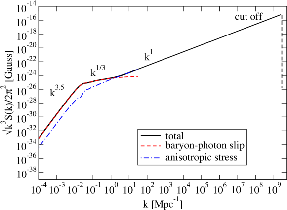
Figure 6: Spectrum of magnetic fields generated from cosmological density perturbations at $z=1100$. Red dashed line shows contribution from baryon photon slip, blue dash-dotted line from anisotropic stress of photons, and black like shows the total spectrum. The spectrum was obtained by direct numerical integration up to k=30 Mpc^-1, and by analytic extrapolation above it. The spectrum has a slope proportional to $k^{3.5}$ at larger scale than the horizon at recombination. At smaller scales than $\sim$1 Mpc^-1, magnetic fields are dominated by the contribution from the anisotropic stress of photons. At smallest scale around $2\times 10^{-3}$ pc, the spectrum would have a cut-off due to the relativistic effects of electrons (and positrons).

We depict the spectrum of magnetic fields in Fig. 6. By remembering the fact that the spectrum of magnetic field $S(k)$ is proportional to $P(k)P(k-k^{\prime})$, the spectrum can be easily generalized in the case of tilted spectrum:

$$B\propto\sqrt{k^{3}S(k)}\propto\left\{\begin{array}[]{rll}&k^{3.5}&\mbox{\hskip 28.45274pt(\phantom{$10$ ~{}Mpc$\mathrel{\mathchoice{\lower 3.6pt\vbox{\halign{$\mathsurround=0pt\displaystyle\hfil#\hfil$\cr<\crcr\sim\crcr}}}{\lower 3.6pt\vbox{\halign{$\mathsurround=0pt\textstyle\hfil#\hfil$\cr<\crcr\sim\crcr}}}{\lower 3.6pt\vbox{\halign{$\mathsurround=0pt\scriptstyle\hfil#\hfil$\cr<\crcr\sim\crcr}}}{\lower 3.6pt\vbox{\halign{$\mathsurround=0pt\scriptscriptstyle\hfil#\hfil$\cr<\crcr\sim\crcr}}}}$ }$\lambda\mathrel{\mathchoice{\lower 3.6pt\vbox{\halign{$\mathsurround=0pt\displaystyle\hfil#\hfil$\cr>\crcr\sim\crcr}}}{\lower 3.6pt\vbox{\halign{$\mathsurround=0pt\textstyle\hfil#\hfil$\cr>\crcr\sim\crcr}}}{\lower 3.6pt\vbox{\halign{$\mathsurround=0pt\scriptstyle\hfil#\hfil$\cr>\crcr\sim\crcr}}}{\lower 3.6pt\vbox{\halign{$\mathsurround=0pt\scriptscriptstyle\hfil#\hfil$\cr>\crcr\sim\crcr}}}}100$ Mpc)}\\ &k^{n_{s}-2/3}&\mbox{\hskip 28.45274pt($10$ ~{}Mpc$\mathrel{\mathchoice{\lower 3.6pt\vbox{\halign{$\mathsurround=0pt\displaystyle\hfil#\hfil$\cr<\crcr\sim\crcr}}}{\lower 3.6pt\vbox{\halign{$\mathsurround=0pt\textstyle\hfil#\hfil$\cr<\crcr\sim\crcr}}}{\lower 3.6pt\vbox{\halign{$\mathsurround=0pt\scriptstyle\hfil#\hfil$\cr<\crcr\sim\crcr}}}{\lower 3.6pt\vbox{\halign{$\mathsurround=0pt\scriptscriptstyle\hfil#\hfil$\cr<\crcr\sim\crcr}}}}\lambda\mathrel{\mathchoice{\lower 3.6pt\vbox{\halign{$\mathsurround=0pt\displaystyle\hfil#\hfil$\cr<\crcr\sim\crcr}}}{\lower 3.6pt\vbox{\halign{$\mathsurround=0pt\textstyle\hfil#\hfil$\cr<\crcr\sim\crcr}}}{\lower 3.6pt\vbox{\halign{$\mathsurround=0pt\scriptstyle\hfil#\hfil$\cr<\crcr\sim\crcr}}}{\lower 3.6pt\vbox{\halign{$\mathsurround=0pt\scriptscriptstyle\hfil#\hfil$\cr<\crcr\sim\crcr}}}}100$ Mpc)}\\ &k^{n_{s}}&\mbox{\hskip 28.45274pt($10^{-3}$~{} pc$\mathrel{\mathchoice{\lower 3.6pt\vbox{\halign{$\mathsurround=0pt\displaystyle\hfil#\hfil$\cr<\crcr\sim\crcr}}}{\lower 3.6pt\vbox{\halign{$\mathsurround=0pt\textstyle\hfil#\hfil$\cr<\crcr\sim\crcr}}}{\lower 3.6pt\vbox{\halign{$\mathsurround=0pt\scriptstyle\hfil#\hfil$\cr<\crcr\sim\crcr}}}{\lower 3.6pt\vbox{\halign{$\mathsurround=0pt\scriptscriptstyle\hfil#\hfil$\cr<\crcr\sim\crcr}}}}\lambda\mathrel{\mathchoice{\lower 3.6pt\vbox{\halign{$\mathsurround=0pt\displaystyle\hfil#\hfil$\cr<\crcr\sim\crcr}}}{\lower 3.6pt\vbox{\halign{$\mathsurround=0pt\textstyle\hfil#\hfil$\cr<\crcr\sim\crcr}}}{\lower 3.6pt\vbox{\halign{$\mathsurround=0pt\scriptstyle\hfil#\hfil$\cr<\crcr\sim\crcr}}}{\lower 3.6pt\vbox{\halign{$\mathsurround=0pt\scriptscriptstyle\hfil#\hfil$\cr<\crcr\sim\crcr}}}}10~{}~{}$ Mpc)}\\ &\sim 0&\mbox{\hskip 28.45274pt(\phantom{$10$ ~{}Mpc$\mathrel{\mathchoice{\lower 3.6pt\vbox{\halign{$\mathsurround=0pt\displaystyle\hfil#\hfil$\cr<\crcr\sim\crcr}}}{\lower 3.6pt\vbox{\halign{$\mathsurround=0pt\textstyle\hfil#\hfil$\cr<\crcr\sim\crcr}}}{\lower 3.6pt\vbox{\halign{$\mathsurround=0pt\scriptstyle\hfil#\hfil$\cr<\crcr\sim\crcr}}}{\lower 3.6pt\vbox{\halign{$\mathsurround=0pt\scriptscriptstyle\hfil#\hfil$\cr<\crcr\sim\crcr}}}}$ }$\lambda\mathrel{\mathchoice{\lower 3.6pt\vbox{\halign{$\mathsurround=0pt\displaystyle\hfil#\hfil$\cr<\crcr\sim\crcr}}}{\lower 3.6pt\vbox{\halign{$\mathsurround=0pt\textstyle\hfil#\hfil$\cr<\crcr\sim\crcr}}}{\lower 3.6pt\vbox{\halign{$\mathsurround=0pt\scriptstyle\hfil#\hfil$\cr<\crcr\sim\crcr}}}{\lower 3.6pt\vbox{\halign{$\mathsurround=0pt\scriptscriptstyle\hfil#\hfil$\cr<\crcr\sim\crcr}}}}10^{-3}$ pc)}\end{array}\right.$$ (90)

where $n_{s}$ is the spectral index of primordial density perturbations.

V Magnetic Helicity

So far, we have investigated the spectrum of magnetic field amplitude while there exists another important quantity, helicity, which defines the property of stochastic magnetic fields. Magnetic helicity is a quantity which characterizes magnetic field configuration how much the magnetic field lines are twisted, or how many closed magnetic lines are linked Biskamp (1993). Among the cosmological mechanisms to generate magnetic fields, a number of scenarios predicts the primordial fields with non-zero helicity Vachaspati (2001); Field and Carroll (2000); Semikoz and Sokoloff (2005). Therefore, helicity, as well as amplitude, can be an important probe of the origin of primordial magnetic fields.

Since magnetic helicity is a conserved quantity in the limit of infinite conductivity in the standard MHD theory, it should remain zero if there was no helicity initially in the early universe. To generate cosmological magnetic fields with non-zero helicity, parity violating processes would be necessary, often related with CP violation of fundamental particle interactions. This will lead us to the conclusion that helicity can not be generated if magnetic fields were generated through density perturbations where the standard Compton scatterings are the only relevant particle interactions. In fact, we can explicitly show that magnetic fields generated from cosmological perturbation discussed in this paper have no magnetic helicity as follows.

Formally, the magnetic helicity density is defined as

$${\cal H}=\frac{1}{V}\int d^{3}x\vec{A}\cdot\vec{B}~{},$$ (91)

where $\vec{A}$ is the vector potential and $V$ is the normalization volume. Similar to the way to define the magnetic field spectrum $S(k)$, the helicity spectrum $P_{H}(k)$ can be defined as

$$\left<A_{i}(\vec{k})B^{\ast}_{j}(\vec{k^{\prime}})\right>=\delta^{(3)}(\vec{k}-\vec{k^{\prime}})P_{ij}(\hat{k})\frac{P_{H}(k)}{2k}~{},$$ (92)

where $P_{ij}(\hat{k})=\delta_{ij}-\hat{k}_{i}\hat{k}_{j}$ is the projection tensor^†. Note that $P_{ij}$ satisfies the divergence-less condition of magnetic fields, $k^{i}P_{ij}=0$. Remembering that $B_{i}=i\epsilon_{ijk}k_{j}A_{k}$, Eq. (92) can be put together with magnetic field spectrum $S(k)$ as

$$\left<B_{i}(\vec{k})B^{\ast}_{j}(\vec{k^{\prime}})\right>=\delta^{(3)}(\vec{k}-\vec{k^{\prime}})\left[P_{ij}(\hat{k})\frac{S(k)}{2}+i\epsilon_{ijl}\hat{k}^{l}\frac{P_{H}(k)}{2}\right]~{}.$$ (93)

Thus, the antisymmetric part of magnetic field correlations denotes helicity of magnetic fields.

To see explicitly that magnetic fields generated from density perturbations have no helicity, let us consider an alternative expression for Eq. (93)

$$\left<B_{j}(\vec{k})B^{\ast}_{i}(\vec{k^{\prime}})\right>=\delta^{(3)}(\vec{k}-\vec{k^{\prime}})\left[P_{ij}(\hat{k})\frac{S(k)}{2}-i\epsilon_{ijl}\hat{k}^{l}\frac{P_{H}(k)}{2}\right]~{},$$ (94)

and subtract this from Eq.(93), which should be zero if there is no magnetic helicity. The magnetic fields generated from cosmological perturbations can be symbolically expressed as

$$B_{i}(\vec{k})=\epsilon^{iab}\int d^{3}\vec{K}\hat{K}_{a}k_{b}f(\vec{K},\vec{k})\delta(\vec{k}-\vec{K})\gamma(\vec{K})~{},$$ (95)

where $f(\vec{K},\vec{k})$ is a real function of $\vec{K}$ and $\vec{k}$ (eq.(55)), and $\delta$ and $\gamma$ are the time integration of perturbation variables. Let us now explicitly evaluate $\left<B_{i}(\vec{k})B_{j}^{\ast}(\vec{k}^{\prime})\right>-\left<B_{j}(\vec{k})B_{i}^{\ast}(\vec{k}^{\prime})\right>$ as

$$\left<B_{i}(\vec{k})B_{j}^{\ast}(\vec{k}^{\prime})\right>-\left<B_{j}(\vec{k})B_{i}^{\ast}(\vec{k}^{\prime})\right> = \delta^{(3)}(\vec{k}-\vec{k}^{\prime})\int d^{3}\vec{K}P(K)P(|\vec{k}-\vec{K}|)f(\vec{K},\vec{k})\epsilon^{iab}\epsilon^{jlm}$$ (96)

$$\times \biggl{\{}(\hat{K}_{a}k_{b}\hat{K}_{l}k_{m}-\hat{K}_{l}k_{m}\hat{K}_{a}k_{b})f(\vec{K},\vec{k})\gamma^{2}(K)\delta^{2}(|\vec{k}-\vec{K}|)$$

$$+ \frac{\left(\hat{K}_{a}k_{b}(k_{l}-K_{l})k_{m}-\hat{K}_{l}k_{m}(k_{a}-K_{a})k_{b}\right)}{|\vec{k}-\vec{K}|}f(\vec{k}-\vec{K},\vec{k})\delta(|\vec{k}-\vec{K}|)\gamma(|\vec{k}-\vec{K}|)\gamma(K)\delta(K)\biggr{\}}$$

$$= 0~{}.$$

Thus, the helical part of magnetic fields from density perturbations should vanish. This fact is in marked contrast to the other origins of primordial magnetic fields in the very early universe (above GeV), where the magnetic fields must be somewhat helical due to the interaction of the magnetic field with a cosmic axion field Campanelli and Giannotti (2005).

Several ways to detect helicity of magnetic fields have been proposed. It was shown that primordial helicity can be a new source to induce parity-odd correlations such as between temperature anisotropy and B-mode polarization, and that between E-mode and B-mode polarizations in CMB anisotropies Pogosian et al. (2002); Caprini et al. (2004); Kahniashvili and Ratra (2005), which are zero for fields without any helicity. Recently, Kahniashvili and Vachaspati proposed that the correlation of the arrival momenta of the cosmic rays can be used to detect helicity of an intervening magnetic field Kahniashvili and Vachaspati (2006). Although it is very difficult to detect helicity in the cosmological magnetic fields, yet it deserves further investigations since detecting helicity will shed light on the mystery of the origin of large-scale magnetic fields.

VI discussion and summary

In this paper we discussed a generation mechanism of magnetic fields from cosmological density perturbations. Following our previous papers, we present a detailed formulation for the magnetic field generation. The key is that photons scatter off only electrons (and not protons) by Compton scatterings. Electric fields are induced to prevent charge separation between electrons and protons, and magnetic fields are generated from these induced electric fields through Maxwell equations. We showed that the baryon-photon slip and the anisotropic stress of photons can generate the magnetic fields if second order couplings in density perturbations are taken into account when evaluating Compton scattering terms. Since these two sources for magnetic fields naturally arise from density perturbations for a wide range of wavenumbers, the fields are also naturally generated for a wide range of scales. We then gave an analytic interpretation of the resultant spectrum of magnetic fields within the framework of the cosmological perturbation theory. Using the tight-coupling approximation of baryon-photon plasma, we showed that the fields have the spectrum $\sqrt{k^{3}S(k)}\propto k$ at small scales where the photon anisotropic stress is the dominant contributor, and thus the fields become stronger at smaller scales. A typical amplitude of magnetic fields is of the order $10^{-24}$ Gauss at 1 Mpc scale. Magnetic helicity should not be associated with these magnetic fields. We also found that magnetic fields have a cut-off around $2\times 10^{-3}$ pc due to the relativistic effects of electrons.

In our previous papers Takahashi et al. (2005); Ichiki et al. (2006) we suggested that the magnetic fields as strong as $10^{-18}$ Gauss can arise at Mpc scale at recombination, which is larger than the amplitude presented in this paper. The main difference from the previous results comes from the missing scale factor in equation (49). This mistake leads an overall overestimate for the magnetic field amplitude and a steeper magnetic field spectrum on small scales, where the fields are mainly created at earlier epochs. The amplitude obtained here is widely consistent with recent literatures around a comoving scale of $0.1$ Mpc^-1 Matarrese et al. (2005); Gopal and Sethi (2005); Siegel and Fry (2006). However, there still exists the difference of the amplitude of magnetic fields at smaller scales. For example, our results show stronger magnetic fields by the factor of $10^{2}$ than those reported in Matarrese et al. (2005); Siegel and Fry (2006) at Mpc comoving scale, and the difference becomes even larger at smaller scales. This may be because they have evaluated the strength of magnetic fields at the instance of recombination at which the Silk damping effect have already erased perturbations on scales smaller than $k\sim 0.1$ Mpc^-1, while we have solved the evolution equation of magnetic fields from deep in the radiation epoch, through matter-radiation equality, to recombination. In ref. Berezhiani and Dolgov (2004), it is also discussed that larger magnetic fields arise at small scales if one consider the earlier period. It is natural to consider that magnetic fields generated prior to recombination can survive, because the diffusion scale in the highly conductive primordial plasma due to the Ohmic dissipation is much smaller than cosmological scales considered here. Therefore, we think that magnetic fields generated from (nearly scale invariant) density perturbations should dominate on small scales. We will give further details about the discrepancy between our work and others elsewhere soon Takahashi et al. (2006).

As discussed in this paper, magnetic fields have a small scale power up to $2\times 10^{-3}$ pc comoving scale. This scale corresponds to the cosmic horizon when the temperature of the universe was around MeV. Until this epoch, thermally created electrons and positrons significantly suppressed the sources of magnetic fields. If we assume the scale invariant spectrum for primordial density perturbations, our results indicate that magnetic fields as strong as $\sim 10^{-15}$ Gauss can arise at this scale. Although these are small compared with the micro Gauss fields observed in present galaxies, it would be enough for the hydro-dynamical dynamo action to amplify into the present amplitude during the structure formation until today Davis et al. (1999). Of course, if density perturbations have a blue spectrum, or they are anomalously large at small scales Kawasaki et al. (2006) larger magnetic fields will be generated.

Although cosmologically generated magnetic fields appear sufficient for ’seed fields’ of galactic magnetic fields, it is still unclear whether they can act as seed magnetic fields for galaxy clusters. In most astrophysical objects, such as disk galaxies and stars, differential rotation is important for amplifying and sustaining their own magnetic fields. However, galaxy clusters have little rotation, and therefore, another mechanisms will be necessary. It is recently argued that cluster plasmas threaded by weak magnetic fields are subject to very fast growing instabilities, and this instability happens once the ions are magnetized Schekochihin et al. (2005). The magnetized condition corresponds to the magnetic field amplitude of $10^{-18}$ G for typical cluster parameters, which is a little larger than that of cosmologically generated seed fields which we found here. Furthermore, the fields amplified by plasma instabilities have a rather small reversal scale (typically $10^{4}$ km to 10pc Schekochihin and Cowley (2006)), while the observational data suggest that the typical reversal scale is $\sim 1$ kpc. Therefore we can not conclude that magnetic fields in clusters of galaxies can directly arise from the seed fields generated from density perturbations in the early universe.

To observe these seed magnetic fields in a direct manner is interesting but very challenging. The magnetic fields at recombination should leave an imprint on CMB photons through Faraday rotation. Faraday rotation can then create B-mode polarization from the dominant E-mode polarization which associates with (scalar) density perturbations. Furthermore, sufficiently large magnetic fields can source the vector mode perturbations on baryon fluid by themselves, which then induce B-mode polarization pattern in CMB Yamazaki et al. (2005); Lewis (2004). By analyzing polarization patterns at large scales one can in principle get rid of information about the magnetic fields. Observation forecast predicts that the fields as week as $10^{-10}$ G will be detected by future missions such as Planck, which is however still out of reach of the weak magnetic ’seed’ field created from density perturbations discussed here.

Another promising way to detect the weakest ’seed’ magnetic fields would be to measure the time-delayed emissions from the gamma-ray bursts. The idea was originally proposed by Plaga Plaga (1995), and there the author concluded that magnetic fields as week as $10^{-24}$ Gauss in void regions can be probed by detecting time-delayed events of GeV-TeV photons. Of course one may claim that it is highly uncertain whether magnetic fields in void regions purely consist of the remnant seed fields created in the early universe. Interestingly, it is argued that large volume of void regions can escape from any astrophysical activities such as galactic winds Bertone et al. (2006). Therefore, it is likely that one can probe primordial magnetic fields by measuring void fields through gamma-ray photons. Unfortunately, it would be impossible to reach the field as weak as $10^{-24}$ Gauss in practice, because there exist another effects to cause time delays to high energy gamma-ray photons. Subsequent studies have shown that magnetic fields strength as strong as $10^{-19}$ G would be necessary for time-delays by magnetic deflection to be longer than those caused by angular spreading Razzaque et al. (2004). Therefore, it appears that an amplification of ’seed’ magnetic fields at recombination by at least $\sim$ 100 will be necessary for the fields to lead any observational signatures in gamma-ray photons. Clearly it will be of great interest to study the evolution of magnetic fields in the void regions from recombination to the present universe.