The impact of dipole straylight contamination on the alignment of low multipoles of CMB anisotropies

Abstract

We estimate the impact of the Dipole Straylight Contamination (DSC) for the Planck satellite on the alignments of vectors associated to the low multipoles of the pattern of the cosmic microwave background (CMB) anisotropies. In particular we study how the probability distributions of eighteen estimators for the alignments change when DSC is taken into account. We find that possible residual DSC should leave a non-negligible impact on low multipole alignments for effective values of the fractional far sidelobe integrated response, $p$, larger than $\sim{\rm few}\times 10^{-3}$. The effect is strongly dependent on the intrinsic sky amplitude and weakly dependent on the considered scanning strategy. We find a decrease of the alignment probability between the quadrupole and the dipole and an increase of the alignment probability between the hexadecapole and the dipole (larger is the intrinsic sky amplitude and lower is the contamination). The remaining estimators do not exhibit clear signatures, except, in some cases, considering the largest values of $p$ and the lowest sky amplitudes. Provided that the real sidelobes of the Planck receivers in flight conditions will correspond to $p\,\lower 2.0pt\hbox{${<\atop\hbox{\raise 4.0pt\hbox{$\sim$}}}$}\,{\rm few}\times 10^{-3}$, as realistically expected at least in the cosmological frequency channels, and will be known with accuracies better than $\sim{\rm few}\times 10$% allowing for a suitable cleaning during data reduction, Planck will be very weakly affected from DSC on the alignments of low multipoles.

1 Introduction

The anisotropy pattern of the Cosmic Microwave Background (CMB), obtained by Wilkinson Microwave Anisotropy Probe (WMAP), probes cosmological models with unprecedented precision (Spergel et al., 2006). Although WMAP data are largely consistent with the concordance $\Lambda$ Cold Dark Matter ($\Lambda$CDM) model, there are some interesting deviations from it, in particular on the largest angular scales: a surprisingly low amplitude of the quadrupole term of the angular power spectrum (APS), found by Cosmic Background Explorer (COBE) (Smoot et al., 1990; Hinshaw et al., 1996) and WMAP (Spergel et al., 2006), and an unlikely (for a statistically isotropic random field) alignment of the quadrupole and the octupole (Tegmark, de Oliveira Costa and Hamilton, 2003; Copi et al., 2004; Schwarz et al., 2004; Land & Magueijo, 2005a; Vale, 2005; Weeks, 2005; Copi et al., 2006; Abramo et al., 2006). Moreover, both quadrupole and octupole align with the CMB dipole. Other unlikely alignments are present in the aforementioned papers and other low $\ell$ anomalies are described in Eriksen et al. (2004).

It is still unknown if these anomalies come from fundamental physics or if they are the residual of some not removed astrophysical or systematic effect. This open question has attracted a lot of interest and many papers have been published about this subject in the last few years.

This paper represents a step forward of a previous work (Burigana, Gruppuso & Finelli (2006), henceforth BGF06) where the impact of the systematic effect induced by the CMB kinematic dipole signal entering the main spillover (Dipole Straylight Contamination, DSC) on the APS has been studied in particular for the forthcoming Planck mission. Here we wish to estimate the main implications of the same systematic effect on the issue of alignments of the low multipole vectors under experimental conditions (observational strategy, main properties of the far sidelobes) like those typically predicted for Planck in its cosmological frequency channels (at the lowest and highest Planck frequency channels Galactic straylight dominates over dipole straylight).

The measurement of the low $\ell$ pattern is affected by cosmic variance, foregrounds and systematic effects [for a discussion on Galactic straylight contamination see e.g. Burigana et al. (2001, 2004) and Sandri et al. (2004) in the context of the Planck Low Frequency Instrument (LFI) (Mandolesi et al., 1998), Lamarre et al. (2002) in the context of the Planck High Frequency Instrument (HFI) (Puget et al., 1998), and Barnes et al. (2003), Chiang, Coles & Naselsky (2006), in the context of WMAP; see e.g. Chiang, Naselsky & Coles (2006); Naselsky & Verkhodanov (2006) for an analysis of large angular scale foreground contamination in WMAP data].

Through a simple analytical model [top-hat approximation for the main spillover response (Gruppuso, Burigana & Finelli, 2006)] and several numerical simulations we tackled the systematic effect induced on the APS at low and intermediate multipoles by the CMB kinematic dipole signal entering the main spillover (BGF06). In that study, we analytically found that in one survey or in an odd number of surveys the DSC map, described by the coefficients $a_{\ell m}^{SL}$, that turn on for $\ell\leq 4$, is given by

$$a_{10}^{SL}=2\sqrt{4\pi\over 3}c_{1}\alpha\,,$$ (1.1)

$$a_{1\pm 1}^{SL}={1\over 2}{8\pi\over 3}\left(\pm d_{1}+id_{2}\right)c_{23}\alpha\,,$$ (1.2)

for the dipole,

$$a_{2\pm 2}^{SL}=-\left(4\over 3\right)^{2}\sqrt{15\over 32\pi}\left(d_{1}\pm 2id_{2}\right)c_{23}\,,$$ (1.3)

for the quadrupole and

$$a_{4\pm 2}^{SL}=-{4\over 15}\sqrt{5\over 2\pi}\left(d_{1}\pm 2id_{2}\right)c_{23}\,,$$ (1.4)

$$a_{4\pm 4}^{SL}=-{12\over 225}\sqrt{35\over 2\pi}\left(d_{1}\pm 4id_{2}\right)c_{23}\,,$$ (1.5)

for the hexadecapole, where $c_{23}=c_{2}+c_{3}$ and

$$c_{1}=\sqrt{3/4\pi}\,f_{SL}\Delta\,\sin(2\Delta)\,T_{10}\,,$$ (1.6)

$$c_{2}=4\sqrt{3/8\pi}\,f_{SL}\,\Delta\,,$$ (1.7)

$$c_{3}=4\sqrt{3/8\pi}\,f_{SL}\,\sin(2\Delta)/2\,,$$ (1.8)

$$d_{1}=\sin\Delta\,Re\left[T_{11}\right]\,,$$ (1.9)

$$d_{2}=\sin\Delta\,Im\left[T_{11}\right]\,,$$ (1.10)

with $f_{SL}=p/(4\Delta\sin\Delta)$, $p$ being the ratio between the power entering the main spillover and the total power entering the receiver (i.e. essentially the power entering the main beam) and $\Delta$ being the angular side of the box that in the $(\theta,\varphi)$-plane describe the main spillover region. Note that the octupole is unaffected. The terms $T_{10}$, $Re\left[T_{11}\right]$ and $Im\left[T_{11}\right]$ are the coefficients of the kinematic dipole. In ecliptic coordinates their values in thermodynamic temperature are

$$Im\left[T_{11}\right]=0.69823\,{\rm mK}\,,$$ (1.11)

$$T_{10}=-1.32225\,{\rm mK}\,,$$ (1.12)

$$Re\left[T_{11}\right]=4.69963\,{\rm mK}\,.$$ (1.13)

The expressions for $a_{\ell m}^{SL}$ are obtained perturbatively to the first order in the angle ($\alpha$) between the directions of the main spillover and of the spin axis. Moreover, it has been supposed that the main spillover centre is located on the plane defined by the spin axis and the telescope line of sight ($\theta_{mb}$,$\varphi_{mb}$). The relaxation of the latter assumption is described by the introduction of a phase $\beta$ that parametrize the displacement of the main spillover direction from $\theta_{mb}$. The above expressions hold in the case of a simple scanning strategy with the spacecraft spin axis always on the ecliptic plane, i.e., in the case of Planck, for the so-called nominal scanning strategy (NSS) (Dupac & Tauber, 2005). The treatment of complex scanning strategies require numerical simulations.

Note the simple pattern at low $\ell$ due to DSC: even multipoles are modified at the leading order in $\alpha$ whereas odd multipoles do not change or are only weakly contaminated (i.e. linearly in $\alpha$). The introduction of $\beta$ does not change this scheme and $\beta$ appears only to the linear order in $\alpha$ in the odd multipoles (BGF06). Therefore, for the dipole the introduction of $\beta$ leads to the replacements

$$a_{10}^{SL}\rightarrow a_{10}^{SL}\cos\beta+{8\over 3}\sqrt{3\over 4\pi}d_{2}c_{23}\alpha\sin\beta\,,$$ (1.14)

$$a_{1\pm 1}^{SL}\rightarrow a_{1\pm 1}^{SL}\cos\beta+{16\over 3}\sqrt{3\over 2\pi}c_{1}i\alpha\sin\beta\,.$$ (1.15)

In addition, for the octupole we have the following non vanishing coefficients

$$a_{3\pm 2}^{SL}=-{2\over 3}\sqrt{14\over 15\pi}\left(\pm 2id_{1}+d_{2}\right)c_{23}\alpha\sin\beta\,,$$ (1.16)

$$a_{3\pm 3}^{SL}={16\over 9}\sqrt{7\over 5\pi}ic_{1}\alpha\sin\beta\,.$$ (1.17)

In order to investigate the implications of a non-proper subtraction of DSC on the low $\ell$ alignments for the Planck experiment, we consider not only the above summarized analytical description (where the NSS is adopted) but also numerical simulations to explore the case of a cycloidal scanning strategy (CSS) (with slow precessions) that is beyond the analytical approximation.

We shall consider the case of a single survey (or of an odd number of surveys), so providing upper limits to the contamination induced by this effect. Except for the dipole, the final DSC impact is in fact significantly reduced by considering an even number of complete surveys, although in a way dependent on the considered scanning strategy (we remember that also in the case of an even number of surveys a remarkable effect survives to the averaging if one survey is not complete).

This article is organized as follows. In Section 2 the multipole vectors expansion and its link with spherical harmonic expansion is reviewed along the line suggested by Weeks (2005) discussing also the complementarity between the information contained in the APS and in the multipole vectors. In Section 3 we describe the simulations that we have performed and how the estimators for the statistical analysis are defined. In Section 4 we present how the probability distribution of the estimators change when DSC is taken into account. Finally, we discuss the obtained results and draw our conclusions in Section 5.

2 Multipole Vectors

The alignment of multipoles is better understood by a new representation of CMB anisotropy maps where the $a_{\ell m}$ (coefficients of the expansion over the basis of spherical harmonics) are replaced by vectors (Copi et al., 2004). In particular, each multipole order $\ell$ is represented by $\ell$ unit vectors and one amplitude $A$

$$a_{\ell m}\leftrightarrow A^{(\ell)},\hat{u}_{1},\,\cdot\cdot\cdot\,,\hat{u}_{\ell}\,.$$ (2.18)

Note that the number of independent objects is the same in the l.h.s and r.h.s. of equation (2.18): $2\ell+1$ for $a_{\ell m}$ equals $3\ell$ (numbers of components of the vectors) $+1$ (given by $A^{(\ell)}$) $-\ell$ (because there are $\ell$ constraints due to the normalization conditions of the vectors). One of the advantage of this representation is that from these unit vectors one can easily construct scalar quantities that are invariant under rotation. Note that is not equally easy to obtain scalar quantities directly from the $a_{\ell m}$ coefficients that, of course, depend on the coordinate system.

Equation (2.18) can be understood starting from this observation (Weeks, 2005): if $f$ is a solution of the Laplace equation

$$\nabla^{2}f=0\,,$$ (2.19)

where $\nabla^{2}=\partial_{x}^{2}+\partial_{y}^{2}+\partial_{z}^{2}$ in Cartesian coordinates, then it is possible to build a new solution $f^{\prime}$ applying a directional derivative to $f$

$$\nabla_{\vec{u}}f\equiv\vec{u}\cdot\nabla f=f^{\prime}\,,\;\;\;\;\;\;\nabla^{2}f^{\prime}=0\,,$$ (2.20)

with the gradient $\nabla=(\partial_{x},\partial_{y},\partial_{z})$. This happens because the two operators $\nabla^{2}$ and $\nabla_{\vec{u}}$ commute. Maxwell (1873) repeated this observation $\ell$ times considering the $1/r$ potential as starting solution. Here $\vec{r}=(x,y,z)$ and $r=\sqrt{\vec{r}\cdot\ \vec{r}}=\sqrt{x^{2}+y^{2}+z^{2}}$. In this way, one obtains

$$f_{\ell}(x,y,z)=\nabla_{\vec{u}_{\ell}}\cdots\nabla_{\vec{u}_{2}}\nabla_{\vec{u}_{1}}\;\frac{1}{r}\,.$$ (2.21)

Observe the simple pattern that emerges as we apply the directional derivatives one at a time:

$$f_{0} = \frac{1}{r}$$

$$f_{1} = \frac{(-1)(\vec{u}_{1}\cdot\vec{r})}{r^{3}}$$

$$f_{2} = \frac{(3\cdot 1)(\vec{u}_{1}\cdot\vec{r})(\vec{u}_{2}\cdot\vec{r})+r^{2}(-\vec{u}_{1}\cdot\vec{u}_{2})}{r^{5}}$$

$$f_{3} = \frac{(-5\cdot 3\cdot 1)(\vec{u}_{1}\cdot\vec{r})(\vec{u}_{2}\cdot\vec{r})(\vec{u}_{3}\cdot\vec{r})+r^{2}(...)}{r^{7}}\,.$$

The (…) stands for a polynomial which we do not write explicitly, being useless for the current purposes.

Moreover, writing $f_{\ell}$ in spherical coordinates once $r$ is set to $1$, one finds the following property

$$\tilde{\nabla}^{2}f_{\ell}(1,\theta,\phi)=\ell(\ell+1)f_{\ell}(1,\theta,\phi)\,,$$ (2.22)

where $\tilde{\nabla}^{2}$ is the angular Laplace operator defined as

$$\tilde{\nabla}^{2}=-\left[{1\over\sin\theta}\,\partial_{\theta}\left(\,\sin\theta\,\partial_{\theta}\right)+{1\over\sin^{2}\theta}\,\partial_{\phi}^{2}\right]\,.$$ (2.23)

In other words $f_{\ell}(1,\theta,\phi)$ is eigenfunction of the angular part of the Laplace operator with eigenvalue given by $\ell(\ell+1)$. This is nothing but the definition of spherical harmonics $Y_{\ell,m}$ (Sakurai, 1985). Therefore, for every $\ell$ we can write

$$A^{(\ell)}f_{\ell}(1,\theta,\phi)=\sum_{m=-\ell}^{\ell}a_{\ell m}Y_{\ell m}(\theta,\phi)\,,$$ (2.24)

where the amplitude $A^{(\ell)}$ has been inserted because of normalization. Equation (2.24) makes evident the association represented by equation (2.18). From equation (2.24) it is possible to write down the set of equations that has to be solved to pass from $a_{\ell m}$ to multipole vectors. In order to see that this set is solvable we count the equations and the unknowns involved in this set. From equation (2.24) we have $2\ell+1$ equations (one equation for each independent $a_{\ell m}$ ) plus $\ell$ equations from the normality conditions of the vectors (i.e. $\vec{u}_{i}\cdot\vec{u}_{i}=1$ where $i$ runs from $1$ to $\ell$). Therefore the total number of independent equations is $3\ell+1$. This is also the number of unknowns because we have $3$ unknowns for each vector plus $1$ given by the amplitude $A^{(\ell)}$. This shows that the set is solvable.

Unfortunately, an explicit analytical solution is possible only for $\ell=1$ and for $\ell\neq 1$ numerical method are needed . For $\ell=1$ we have

$$-A^{(1)}(\vec{d}\cdot\vec{r}) = \sum_{m=-1}^{1}a_{1m}Y_{1m}(\theta,\phi)\,,$$ (2.25)

$$\vec{d}\cdot\vec{d} = 1\,.$$ (2.26)

Considering the expression for $Y_{1m}(\theta,\phi)$ (Sakurai, 1985) we have the following analytical solution

$$d_{x} = \mp a_{11}^{(R)}/\sqrt{a_{10}^{2}/2+((a_{11}^{(R)})^{2}+(a_{11}^{(I)})^{2})}\,,$$ (2.27)

$$d_{y} = \pm a_{11}^{(I)}/\sqrt{a_{10}^{2}/2+((a_{11}^{(R)})^{2}+(a_{11}^{(I)})^{2})}\,,$$ (2.28)

$$d_{z} = \pm a_{10}/\sqrt{a_{10}^{2}+2((a_{11}^{(R)})^{2}+(a_{11}^{(I)})^{2})}\,,$$ (2.29)

$$A^{(1)} = \mp{1\over 2}\sqrt{3\over\pi}\sqrt{a_{10}^{2}+2((a_{11}^{(R)})^{2}+(a_{11}^{(I)})^{2})}\,,$$ (2.30)

where $\vec{d}=(d_{x},d_{y},d_{z})$ and the labels $(R)$ and $(I)$ stand for real and imaginary part.

An elegant way of solving numerically the above set of equations (in order to obtain the multipole vectors expansion from the set of $a_{\ell m}$) is presented in Katz & Weeks (2004) and in Weeks (2005) where the problem of finding $\ell$ vectors is translated into the problem of finding the zeros of a polynomial of degree $2\ell$. This method has been implemented in a code developed by Weeks (2005) whose use is aknowledged.

We end this section with two observations:

• equation (2.24) is invariant under the change of sign of an even number of $\vec{u}_{i}$ or under the change of sign of an odd number of $\vec{u}_{i}$ and $A^{(\ell)}$ (Abramo et al., 2006; Katz & Weeks, 2004). This “reflection symmetry” implies that in fact multipole vectors define only directions. Of course the same symmetry has to be satisfied by quantities defined through the multipole vectors. Hence the estimators introduced in Section 3, are sensitive only to directions of multipole vectors (or in other words, they are invariant under change of the sign of the vectors). Notice the ambiguity of sign for the dipole in equations  (2.27-2.30) as an example of the above mentioned reflection symmetry.

• equation (2.24) is also invariant under the trasformation

  $$a_{\ell m}\rightarrow c\,a_{\ell m}\,,$$ (2.31)

  $$A^{(\ell)}\rightarrow c\,A^{(\ell)}\,,$$ (2.32)

  where $c$ is a constant. Therefore the $\ell$ multipole vectors associated to $a_{\ell m}$ are the same as those that are associated to $ca_{\ell m}$. This means that for a sufficiently large number N of random extractions of the $2\ell+1$ independent values of $a_{\ell m}$, the corresponding N sets of $\ell$ multipole vectors do not depend on $C_{\ell}$, the variance of $a_{\ell m}$, in the remarkable case in which the $a_{\ell m}$ follow a Gaussian distribution . As a consequence, the same applies to the estimators for the alignments (see Section 3). For instance if $a_{\ell m}$ follow a Gaussian distribution, the information contained in the multipole vectors is “orthogonal” to that contained in the APS. This property is broken in the presence of a systematic effect altering the above symmetry. In this case the global effect could depend on the intrinsic value of $C_{\ell}^{sky}$. In particular, if not fully removed, DSC will provide a spurious deviation from Gaussianity.

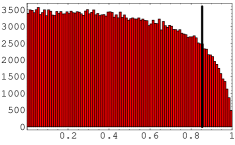
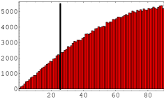
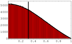
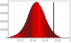
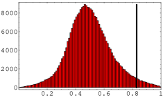
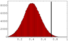
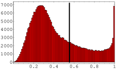
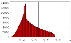
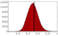
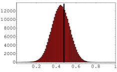
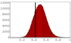
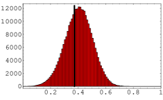
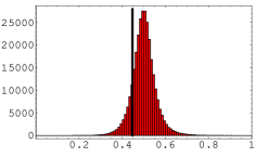
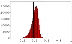
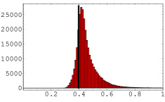
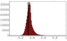
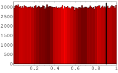
Figure 1: Uncontaminated distribution for all the considered estimators. In order from left to right and above to below: $\hat{W}2$, $W2$, $W2^{\circ}$, $R22$, $\hat{W}3$, $W3$, $D23$, $S23$, $D33$, $S33$, $\hat{W}4$, $W4$, $D42$, $S42$, $D43$, $S43$, $D44$, $S44$. All the panels present the counts ($y$-axis) versus the statistic ($x$-axis). Vertical lines stand for WMAP value reported in Table 1. For $R22$ we overplot the analytic distribution. See also the text.

Estimator WMAP value Probability % $\hat{W}2$ $0.901$ $9.96$ $W2^{\circ}$ $25.68^{\circ}$ $9.94$ $W2$ $0.854$ $8.33$ $R22$ $0.319$ $48.04$ $\hat{W}3$ $0.796$ $3.92$ $W3$ $0.735$ $2.03$ $D23$ $0.829$ $2.74$ $S23$ $0.732$ $0.96$ $D33$ $0.554$ $27.49$

Estimator WMAP value Probability % $S33$ $0.480$ $21.76$ $\hat{W}4$ $0.528$ $38.73$ $W4$ $0.479$ $36.01$ $D42$ $0.422$ $76.82$ $S42$ $0.373$ $62.80$ $D43$ $0.447$ $86.43$ $S43$ $0.384$ $69.75$ $D44$ $0.397$ $82.03$ $S44$ $0.330$ $68.70$

Table 1: WMAP values for the considered estimators adopting the CMB component in the V band of the WMAP 3 year release (see the text for further detailes). The percentages are the probability that a random map would have values for the estimators larger than those observed in the V band by WMAP. Only for $W2^{\circ}$ the percentage represents the probability to extract randomly a value lower than that obtained from the above mentioned data set.

3 Analysis

In order to study the effect of DSC on the alignment of low multipole vectors we have extracted $3\times 10^{5}$ sky realizations for two different APS amplitudes corresponding to a concordance $\Lambda$CDM model and to WMAP. In other words, we have extracted $a_{\ell m}^{sky}$ for $\ell=2$, $\ell=3$ and $\ell=4$ from a Gaussian distribution with zero mean and variance given by $C_{2}$, $C_{3}$, $C_{4}$ and each extraction has been contaminated by $a_{\ell m}^{SL}$. In particular defining $\Delta T_{\ell}=\ell(\ell+1)C_{\ell}/(2\pi)$ we have taken $\Delta T_{2}=1250\,\mu$K², $\Delta T_{3}=1150\,\mu$K² and $\Delta T_{4}=1110\,\mu$K² for the $\Lambda$CDM case and $\Delta T_{2}=211\,\mu$K², $\Delta T_{3}=1041\,\mu$K² and $\Delta T_{4}=731\,\mu$K² for the WMAP-like amplitude case (Hinshaw et al., 2006). Moreover, we set $\beta=0$ for sake of simplicity and considered $p=1/1000,4/1000,7/1000,10/1000$, i.e. in a range representative of current CMB anisotropy space experiments like WMAP and Planck (see e.g. Barnes et al. (2003) and Sandri et al. (2004)). The other parameters are freezed to the following values $\alpha=\pi/18$, $\Delta=\pi/10$, for sake of simplicity. The coefficients $a_{\ell m}^{sky}$ and $a_{\ell m}^{sky}+a_{\ell m}^{SL}$ are then transformed to multipole vectors through the Weeks’ code.

As written above, not only the analytical expressions for $a_{\ell m}^{SL}$ have been used to describe DSC but also numerical simulations have been performed in order to consider cases beyond the analytical approximations. In particular, we have numerically taken into account the case of a CSS with slow precessions as described for example in Dupac & Tauber (2005), assuming a period $T=6$ months and a semi-amplitude of $10^{\circ}$, and considering $\alpha=10^{\circ}$ and $\beta=60^{\circ}$. In this case, we parametrize the main spillover response according to the Gaussian approximation. With reference to § 3.3 of BGF06, we note that in the remarkable case of pencil beam the top-hat and Gaussian approximations are essentially equivalent for small $\Delta$. Differently, the two cases are not equivalent for general values of $\alpha$. On the other hand, it easily to show that in the case $\alpha=0$ they are equivalent up to second order in $\sigma$ and $\Delta$ provided that $\sigma^{2}=\Delta^{2}/3$ (and $b=p$). We then adopt here this relation to define the beamwidth, $\sigma$, of the main spillover in the Gaussian approximation given the chosen value of $\Delta$ in the top-hat approximation used in the analytical approach.

We present in Section 4 how the distributions of the eighteen estimators change when the DSC is properly taken into account. The considered estimators are: for the alignment quadrupole-dipole

$$W2 = |\vec{q}\cdot\hat{d}|\,,$$ (3.1)

$$\hat{W}2 = |\hat{q}\cdot\hat{d}|\,,$$ (3.2)

$$W2^{\circ} = \arccos(|\hat{q}\cdot\hat{d}|)180/\pi\,,$$ (3.3)

for the self alignment of the quadrupole

$$R22=|\hat{q}_{21}\cdot\hat{q}_{22}|\,,$$ (3.4)

for the alignment octupole-dipole

$$W3 = \sum_{i=1}^{3}|\vec{o}_{i}\cdot\hat{d}|/3\,,$$ (3.5)

$$\hat{W}3 = \sum_{i=1}^{3}|\hat{o}_{i}\cdot\hat{d}|/3\,,$$ (3.6)

for the alignment quadrupole-octupole

$$S23 = \sum_{i=1}^{3}|\vec{q}\cdot\vec{o}_{i}|/3\,,$$ (3.7)

$$D23 = \sum_{i=1}^{3}|\hat{q}\cdot\hat{o}_{i}|/3\,,$$ (3.8)

for the self-alignment of the octupole

$$S33 = \sum_{i=1,j>i}^{3}|\vec{o}_{i}\cdot\vec{o}_{j}|/3\,,$$ (3.9)

$$D33 = \sum_{i=1,j>i}^{3}|\hat{o}_{i}\cdot\hat{o}_{j}|/3\,,$$ (3.10)

for the alignment hexadecapole-dipole

$$W4 = \sum_{i=1}^{6}|\vec{e}_{i}\cdot\hat{d}|/6\,,$$ (3.11)

$$\hat{W}4 = \sum_{i=1}^{6}|\vec{e}_{i}\cdot\hat{d}|/6\,,$$ (3.12)

for the alignment hexadecapole-quadrupole

$$S42 = \sum_{i=1}^{6}|\vec{e}_{i}\cdot\vec{q}|/6\,,$$ (3.13)

$$D42 = \sum_{i=1}^{6}|\hat{e}_{i}\cdot\hat{q}|/6\,,$$ (3.14)

for the alignment hexadecapole-octupole

$$S43 = \sum_{i=1}^{6}\sum_{j=1}^{3}|\vec{e}_{i}\cdot\vec{o}_{j}|/18\,,$$ (3.15)

$$D43 = \sum_{i=1}^{6}\sum_{j=1}^{3}|\hat{e}_{i}\cdot\hat{o}_{j}|/18\,,$$ (3.16)

and for the self-alignment of the hexadecapole

$$S44 = \sum_{i=1,j>i}^{6}|\vec{e}_{i}\cdot\vec{e}_{j}|/15\,,$$ (3.17)

$$D44 = \sum_{i=1,j>i}^{6}|\hat{e}_{i}\cdot\hat{e}_{j}|/15\,,$$ (3.18)

where the symbol “hat” stands for a vector with norm equal to $1$ and where the “area vectors” are defined as

$$\vec{q}=\hat{q}_{21}\times\hat{q}_{22}\,,$$ (3.19)

$$\vec{o}_{1}=\hat{o}_{32}\times\hat{o}_{33}\,,$$ (3.20)

$$\vec{o}_{2}=\hat{o}_{33}\times\hat{o}_{31}\,,$$ (3.21)

$$\vec{o}_{3}=\hat{o}_{31}\times\hat{o}_{32}\,,$$ (3.22)

$$\vec{e}_{1}=\hat{e}_{41}\times\hat{e}_{42}\,,$$ (3.23)

$$\vec{e}_{2}=\hat{e}_{41}\times\hat{e}_{43}\,,$$ (3.24)

$$\vec{e}_{3}=\hat{e}_{41}\times\hat{e}_{44}\,,$$ (3.25)

$$\vec{e}_{4}=\hat{e}_{42}\times\hat{e}_{43}\,,$$ (3.26)

$$\vec{e}_{5}=\hat{e}_{42}\times\hat{e}_{44}\,,$$ (3.27)

$$\vec{e}_{6}=\hat{e}_{43}\times\hat{e}_{44}\,,$$ (3.28)

with $\hat{q}_{2j}$ representing the two normalized multipole vectors ($j=1,2$) associated to the quadrupole, $\hat{o}_{3j}$ representing the three normalized multipole vectors ($j=1,2,3$) associated to the octupole and $\hat{e}_{4j}$ representing the four normalized multipole vectors ($j=1,2,3,4$) associated to the hexadecapole. Notice that all the estimators but $W2^{\circ}\in[0^{\circ},90^{\circ}]$, belong to the interval $[0,1]$ and contain absolute values in order to make them invariant under the reflection symmetry discussed in Section 2. Notice also that $R22$ is the unique estimator whose distribution is analytically known [see Land & Magueijo (2005b),Dennis (2005)]:

$$p(x)=27{(1-x^{2})\over{(x^{2}+3)^{5/2}}}\,,$$ (3.29)

where $x=R22$.

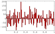
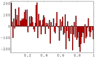
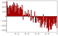
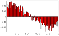
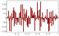
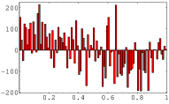
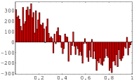
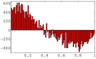
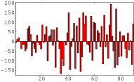
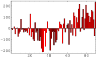
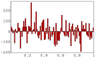
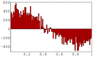
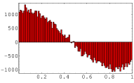
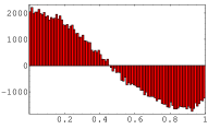
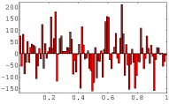
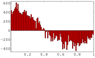
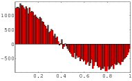
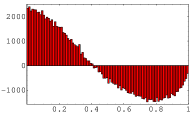
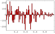
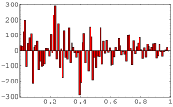
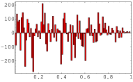
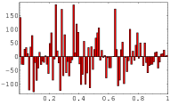
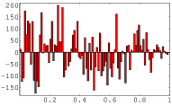
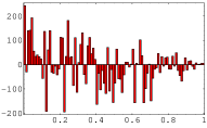
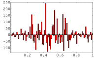
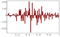
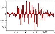
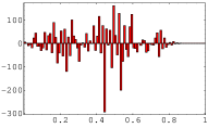
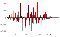
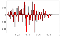
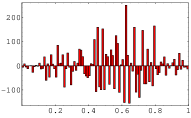
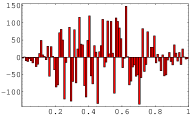
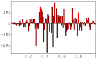
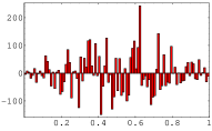
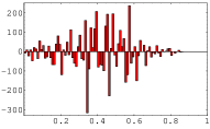
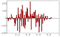
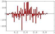
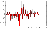
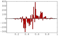
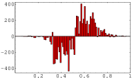
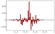
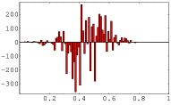
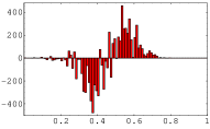
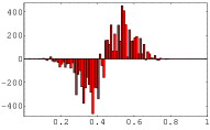
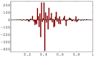
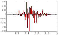
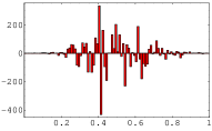
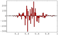
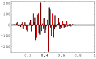
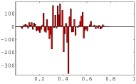
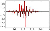
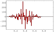
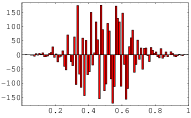
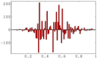
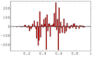
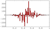
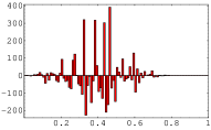
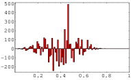
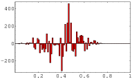
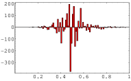
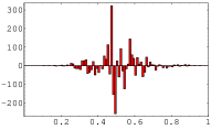
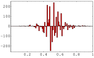
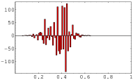
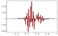
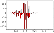
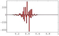
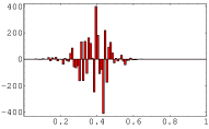
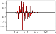
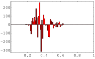
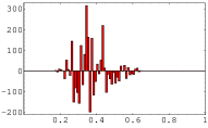
Figure 2: Differences between the DSC contaminated distribution and the uncontaminated one in $\Lambda$CDM model for the alignment Quadrupole-Dipole in the case of small $\alpha$, vanishing $\beta$ and nominal scanning strategy. First row: $\hat{W}2$. Second row: $W2$. Third row: $W2^{\circ}$. From left to right (in every row) $p=1/1000$, $p=4/1000$, $p=7/1000$, $p=10/1000$. All the panels present the counts ($y$-axis) versus the statistic ($x$-axis). See also the text.

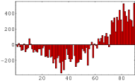
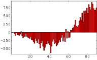
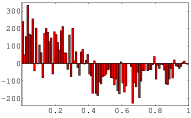
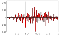
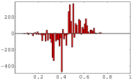
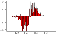
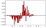
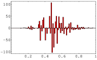
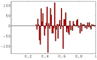
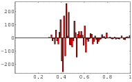
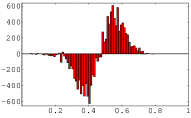
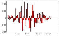
Figure 3: Differences between the DSC contaminated distribution and the uncontaminated one for the WMAP amplitude for the alignment Quadrupole-Dipole in the case of small $\alpha$, vanishing $\beta$ and nominal scanning strategy. First row: $\hat{W}2$. Second row: $W2$. Third row: $W2^{\circ}$. From left to right (in every row) $p=1/1000$, $p=4/1000$, $p=7/1000$, $p=10/1000$. All the panels present the counts ($y$-axis) versus the statistic ($x$-axis). See also the text.

Figure 4: Differences between the DSC contaminated distribution and the uncontaminated one for the self-alignment Quadrupole-Quadrupole in the case of small $\alpha$, vanishing $\beta$ and nominal scanning strategy. First row: $R22$ in $\Lambda$CDM model. Second row: $R22$ for the WMAP amplitude of the intrinsic sky. From left to right (in every row) $p=1/1000$, $p=4/1000$, $p=7/1000$, $p=10/1000$. All the panels present the counts ($y$-axis) versus the statistic ($x$-axis). See also the text.

Figure 5: Differences between the DSC contaminated distribution and the uncontaminated one in $\Lambda$CDM model for the alignment Octupole-Quadrupole in the case of small $\alpha$, vanishing $\beta$ and nominal scanning strategy. First row: $D23$. Second row: $S23$. From left to right (in every row) $p=1/1000$, $p=4/1000$, $p=7/1000$, $p=10/1000$. All the panels present the counts ($y$-axis) versus the statistic ($x$-axis). See also the text.

Figure 6: Differences between the DSC contaminated distribution and the uncontaminated one for the WMAP amplitude for the alignment Octupole-Quadrupole in the case of small $\alpha$, vanishing $\beta$ and nominal scanning strategy. First row: $D23$. Second row: $S23$. From left to right (in every row) $p=1/1000$, $p=4/1000$, $p=7/1000$, $p=10/1000$. All the panels present the counts ($y$-axis) versus the statistic ($x$-axis). See also the text.

4 Results

In Fig. 1 we plot the uncontaminated distribution for $\hat{W}2$, $W2$, $W2^{\circ}$, $R22$, $\hat{W}3$, $W3$, $D23$, $S23$, $D33$, $S33$, $\hat{W}4$, $W4$, $D42$, $S42$, $D43$, $S43$, $D44$, $S44$. Notice the perfect agreement between the analytical, see equation (3.29), and the numerical distribution of $R22$. For sake of completeness we report in Table 1 the values of the considered estimators obtained, for example, adopting the CMB anisotropy component in the V band of the WMAP $3$ year release with a Kp2 mask and the dipole given in Hinshaw et al. (2006).

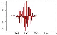
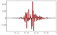
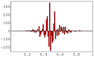
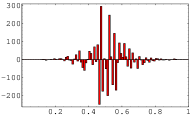
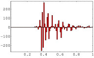
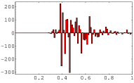
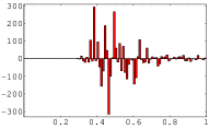
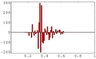
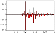
In all the subsequent figures we display the difference (DD) between the distribution contaminated by DSC and the uncontaminated one: Figs 2–14 refer to the considered NSS. The Figures for the considered CSS are not shown being very similar to the NSS. However some (small) differences are reported in Section 5. Of course, the sum of counts of the uncontaminated distribution is always $3\times 10^{5}$ while the sum of counts of the DD is zero.

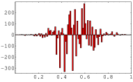
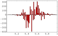
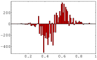
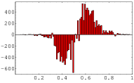
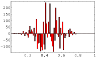
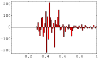
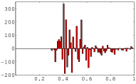
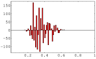
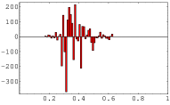
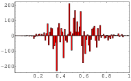
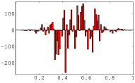
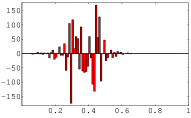
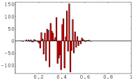
The DD for $\hat{W}2$, $W2$, $W2^{\circ}$ are shown in Fig. 2 for the considered $\Lambda$CDM model and in Fig. 3 for the model with WMAP amplitude. For $\hat{W}3$, $W3$, $D33$ and $S33$ the DD is exactly zero for the considered NSS. Therefore they are not reported for sake of conciseness. For the considered CSS they are noisy-like. The DD for $R22$ are plotted in Fig.4 for the considered $\Lambda$CDM model and for the WMAP amplitude. The DD for $D23$ and $S23$ are shown in Fig. 5 for the considered $\Lambda$CDM model and in Fig. 6 for the WMAP amplitude. The DD for $\hat{W}4$ and $W4$ are plotted in Fig. 7 for the considered $\Lambda$CDM model and in Fig. 8 for the WMAP amplitude. The DD for $D42$ and $S42$ are given in Fig. 9 for the considered $\Lambda$CDM model and in Fig. 10 for the WMAP amplitude. The DD for $D43$ and $S43$ are shown in Fig. 11 for the considered $\Lambda$CDM model and in Fig. 12 for th WMAP amplitude. The DD for $D44$ and $S44$ are plotted in Fig. 13 for the considered $\Lambda$CDM model and in Fig. 14 for the WMAP amplitude. The not reported DD for NSS are essentially noisy-like.

Figure 7: Differences between the DSC contaminated distribution and the uncontaminated one in $\Lambda$CDM model for the alignment Hexadecapole-Dipole in the case of small $\alpha$, vanishing $\beta$ and nominal scanning strategy. First row: $\hat{W}4$. Second row: $W4$. From left to right (in every row) $p=1/1000$, $p=4/1000$, $p=7/1000$, $p=10/1000$. All the panels present the counts ($y$-axis) versus the statistic ($x$-axis). See also the text.

Figure 8: Differences between the DSC contaminated distribution and the uncontaminated one for the WMAP amplitude for the alignment Hexadecapole-Dipole in the case of small $\alpha$, vanishing $\beta$ and nominal scanning strategy. First row: $\hat{W}4$. Second row: $W4$. From left to right (in every row) $p=1/1000$, $p=4/1000$, $p=7/1000$, $p=10/1000$. All the panels present the counts ($y$-axis) versus the statistic ($x$-axis). See also the text.

Figure 9: Differences between the DSC contaminated distribution and the uncontaminated one in $\Lambda$CDM model for the alignment Hexadecapole-Quadrupole in the case of small $\alpha$, vanishing $\beta$ and nominal scanning strategy. First row: $D42$. Second row: $S42$. From left to right (in every row) $p=1/1000$, $p=4/1000$, $p=7/1000$, $p=10/1000$. All the panels present the counts ($y$-axis) versus the statistic ($x$-axis). See also the text.

Figure 10: Differences between the DSC contaminated distribution and the uncontaminated one for the WMAP amplitude for the alignment Hexadecapole-Quadrupole in the case of small $\alpha$, vanishing $\beta$ and nominal scanning strategy. First row: $D42$. Second row: $S42$. From left to right (in every row) $p=1/1000$, $p=4/1000$, $p=7/1000$, $p=10/1000$. All the panels present the counts ($y$-axis) versus the statistic ($x$-axis). See also the text.

Figure 11: Differences between the DSC contaminated distribution and the uncontaminated one in $\Lambda$CDM model for the alignment Hexadecapole-Octupole in the case of small $\alpha$, vanishing $\beta$ and nominal scanning strategy. First row: $D43$. Second row: $S43$. From left to right (in every row) $p=1/1000$, $p=4/1000$, $p=7/1000$, $p=10/1000$.All the panels present the counts ($y$-axis) versus the statistic ($x$-axis). See also the text.

Figure 12: Differences between the DSC contaminated distribution and the uncontaminated one for the WMAP amplitude for the alignment Hexadecapole-Octupole in the case of small $\alpha$, vanishing $\beta$ and nominal scanning strategy. First row: $D43$. Second row: $S43$. From left to right (in every row) $p=1/1000$, $p=4/1000$, $p=7/1000$, $p=10/1000$. All the panels present the counts ($y$-axis) versus the statistic ($x$-axis). See also the text.

5 Discussion and conclusions

In this paper we have studied the impact of a non-proper subtraction of DSC on alignments of multipole vectors associated to low multipoles for the forthcoming Planck mission. This work represents a step forward of BGF06 in the study of DSC on the low multipoles of CMB pattern.

The analyses presented in this paper and in BGF06 provide a working example of a possible connection between the two low $\ell$ anomalies (APS and alignments of the low multipole vectors) in the presence of a non cosmological residual in the data. To our knowledge, a non-properly subtracted systematic effect (of instrumental or astrophysical origin, or, as in this case, coming from a combination of them) represents the easiest way to link the statistics of $a_{\ell m}$ and the amplitude of $C_{\ell}$, otherwise disconnected since the symmetry defined in equations (2.31) and (2.32) holding at least for any distribution writable as in footnote 7 (like the Gaussian one).

We summarize the main results of this paper separately for the considered nominal and cycloidal scanning strategies in the context of the Planck mission (Dupac & Tauber, 2005).

For the NSS:

• the probability of alignment quadrupole-dipole ($\hat{W}2$,$W2$,$W2^{\circ}$) tends to be lowered; the impact of this effect increases going from $\Lambda$CDM-like APS amplitudes to WMAP-like APS amplitudes and for increasing values of $p$, the percentage of power entering the main spillover with respect to the main beam (see Figs 2 and 3);

• some features show up in the estimator for the alignment hexadecapole-dipole ($\hat{W}4$,$W4$) if $p$ is sufficiently large, both for $\Lambda$CDM and WMAP-like amplitudes (see Figs 7 and 8);

• some features show up in the estimator for the alignment hexadecapole-quadrupole ($D42$,$S42$) but only for large $p$, i.e. $p=1/100$, and WMAP-like intrinsic amplitude (see Fig. 10);

• the remaining estimators ($R22$, $D23$, $S23$, $D42$, $S42$, $D43$, $S43$, $D44$, $S44$) do not show remarkable features, being essentially noisy-like (see Figs 5, 9, 11, 12, 13 and 14); on the other hand, a weak signature appears in the case of $R22$, $S23$ and $S44$ (for the alignment octupole-quadrupole and self-alignment of the hexadecapole, respectively) for WMAP-like intrinsic amplitudes and the maximum considered value of $p$ (see Figs 4, 6 and 14).

For the CSS:

• the alignment quadrupole-dipole ($\hat{W}2$,$W2$,$W2^{\circ}$) again tends to be lowered, the impact of this effect being again stronger if the intrinsic sky amplitude is lower and $p$ is sufficiently large ;

• some features appear for the estimator of the alignment hexadecapole-dipole ($\hat{W}4$,$W4$) but stronger than those obtained for the NSS and increasing with $p$ ;

• there is a clear signature in the estimator of the alignment hexadecapole-quadrupole ($D42$,$S42$) but only for WMAP-like amplitudes ;

• again, the remaining estimators ($R22$, $D23$, $S23$, $D43$, $S43$, $D44$, $S44$) do not show remarkable features, being essentially noisy-like; on the other hand, a weak signature appears also for this scanning strategy in the case of $R22$, $S23$ and $S44$ (self alignment of the quadrupole, alignment octupole-quadrupole and self alignment of the hexadecapole respectively), for WMAP-like intrinsic amplitudes and the maximum considered value of $p$.

We conclude that possible residual DSC should leave a non-negligible impact on low multipole alignments for far sidelobe integrated responses corresponding to effective values of $p$ $\,\lower 2.0pt\hbox{${>\atop\hbox{\raise 4.0pt\hbox{$\sim$}}}$}\,{\rm few}\times 10^{-3}$.

We note also that, in general, it could be very useful to carry out the alignment analysis by exploiting both normalized and unnormalized estimators, since they could show different sensitivity in the diagnostic of the same effect, as evident for example in Fig. 5.

The scanning strategy and the behaviour of the optics of WMAP are significantly different from those considered here, suitable for Planck. It is then difficult to extrapolate the above results to the WMAP surveys. If the large scale footprint of the DSC is not so critically dependent on the above details and our analysis applies as well to the WMAP surveys, DSC may not easily explain the whole set of anomalous alignments at large scale found also in WMAP three year release (see Copi et al. (2006)). However, we believe that further studies of this and other systematic effects are required.

Provided that the real sidelobes of the Planck receivers in flight conditions will correspond to values of $p$ $\,\lower 2.0pt\hbox{${<\atop\hbox{\raise 4.0pt\hbox{$\sim$}}}$}\,{\rm few}\times 10^{-3}$ – as realistically expected (Sandri et al., 2004) at least in the cosmological frequency channels – and will be known with relative accuracies better than $\sim{\rm few}\times 10$% (leaving to smaller residual contaminations, equivalent to $p\,\lower 2.0pt\hbox{${<\atop\hbox{\raise 4.0pt\hbox{$\sim$}}}$}\,10^{-3}$, after a suitable cleaning during data reduction) Planck maps will be very weakly affected by DSC on the alignments.

Acknowledgements. We gratefully thank J. Weeks for useful discussions. We warmly acknowledge all the members of the Planck Systematic Effect Working Group for many conversations and collaborations. It is a pleasure to thank D. Maino and P. Naselsky for stimulating conversations. We ackowledge the use of the codes for the computation of multipole vectors provided by Weeks (2005). Some of the results in this paper have been derived using HEALPix (Górski et al., 2005). The use of the WMAP three year release data products is acknowledged. This work has been done in the framework of the Planck LFI activities.

Figure 13: Differences between the DSC contaminated distribution and the uncontaminated one in $\Lambda$CDM model for the self-alignment of the Hexadecapole in the case of small $\alpha$, vanishing $\beta$ and nominal scanning strategy. First row: $D44$. Second row: $S44$. From left to right (in every row) $p=1/1000$, $p=4/1000$, $p=7/1000$, $p=10/1000$. All the panels present the counts ($y$-axis) versus the statistic ($x$-axis). See also the text.

Figure 14: Differences between the DSC contaminated distribution and the uncontaminated one for the WMAP amplitude for the self-alignment of the Hexadecapole in the case of small $\alpha$, vanishing $\beta$ and nominal scanning strategy. First row: $D44$. Second row: $S44$. From left to right (in every row) $p=1/1000$, $p=4/1000$, $p=7/1000$, $p=10/1000$. All the panels present the counts ($y$-axis) versus the statistic ($x$-axis). See also the text.

References

• Abramo et al. (2006) Abramo L.R., Bernui A., Ferreira I.S., Villela T., Wuensche C.A., 2006, Phys. Rev. D, 74, 063506
• Barnes et al. (2003) Barnes C. et al., 2003, ApJS, 148, 51
• Bennet et al. (2003) Bennett C.L. et al., 2003, ApJS, 148, 1
• Burigana et al. (2001) Burigana C., Maino D., Gorski K.M., Mandolesi N., Bersanelli M., Villa F., Valenziano L., Wandelt B.D., Maltoni M., Hivon E., 2001, A&A, 373, 345
• Burigana et al. (2004) Burigana C., Sandri M., Villa F., Maino D., Paladini R., Baccigalupi C., Bersanelli M., Mandolesi N., 2004, A&A, 428, 311
• Burigana, Gruppuso & Finelli (2006) Burigana C., Gruppuso A. and Finelli F., 2006, MNRAS, 371,1570 (BGF06)
• Chiang, Coles & Naselsky (2006) Chiang L.Y., Coles P., Naselsky P.D., Olesen P., 2006, preprint (astro-ph/0608421)
• Chiang, Naselsky & Coles (2006) Chiang L.Y., Naselsky P.D., Coles P., 2006, preprint (astro-ph/0603662)
• Copi et al. (2004) Copi C.J., Huterer D., Starkman G.D., 2004, Phys. Rev. D , 70, 043515
• Copi et al. (2006) Copi C.J., Huterer D., Schwarz D., Starkman G.D., 2006, preprint (astro-ph/0605135)
• Dennis (2005) Dennis M.R., 2005, J.Phys.A: Math.Gen.38, 1653
• Dupac & Tauber (2005) Dupac X. and Tauber J., 2005, A&A, 430, 636
• Eriksen et al. (2004) Eriksen H.K., Hansen F.K., Banday A.J., Gorski K.M., Lilje P.B., 2004, ApJ, 605:14, 2004, Erratum-ibid.609:1198,2004
• GΓ³rski et al. (2005) GΓ³rski K.M., Hivon E., Banday A.J., Wandelt B.D., Hansen F.K., Reinecke M., Bartelman M., 2005, ApJ, 622, 759
• Gruppuso, Burigana & Finelli (2006) Gruppuso A., Burigana C. and Finelli F., 2006, PoS CMB2006:070
• Hinshaw et al. (1996) Hinshaw G. et al., 1996, ApJ, 464, L17
• Hinshaw et al. (2006) Hinshaw G. et al., 2006, preprint (astro-ph/0603451)
• Katz & Weeks (2004) Katz G. and Weeks J., 2004, Phys. Rev. D, 70, 063527
• Lamarre et al. (2002) Lamarre J.M. etΒ al., 2002, in DeΒ Petris M., Gervasi M., eds, AIP Conf. Proc. Vol. 616, Experimental Cosmology at millimetre wavelengths: 2K1BC Workshop. Am. Inst. Phys., New York, p.Β 193
• Land & Magueijo (2005a) Land K. and Magueijo J., 2005a, Phys. Rev. Lett. 95, 071301
• Land & Magueijo (2005b) Land K. and Magueijo J., 2005b, MNRAS, 362, L16-L19
• Mandolesi et al. (1998) Mandolesi N. et al., 1998, PLANCK LFI, A proposal submitted to ESA
• Maxwell (1873) Maxwell J.C., 1873, A Treatise on Electricity and Magnetism reprinted by Dover Publication, 1954
• Naselsky & Verkhodanov (2006) Naselsky P.D., Verkhodanov O.V., 2006, preprint (astro-ph/0609409)
• Puget et al. (1998) Puget J.L. et al., 1998, HFI for the Planck Mission, A proposal submitted to ESA
• Sakurai (1985) Sakurai J.J., 1985, Modern Quantum Mechanics. Revised Edition. Addison-Wesley Publishing Company, Inc.
• Sandri et al. (2004) Sandri M., Villa F., Nesti R., Burigana C., Bersanelli M., Mandolesi N., 2004, A&A, 428, 299
• Schwarz et al. (2004) Schwarz D.J., Starkman G.D., Huterer D., Copi C.J., 2004, Phys. Rev. Lett. 93, 221301
• Smoot et al. (1990) Smoot G.F. et al., 1992, ApJ, 396, L1
• Spergel et al. (2006) Spergel D.N. et al., 2006, preprint (astro-ph/0603449)
• Tegmark, de Oliveira Costa and Hamilton (2003) Tegmark M., de Oliveira Costa A. and Hamilton A., 2003, Phys. Rev. D, 68, 123523
• Vale (2005) Vale C., 2005, preprint (astro-ph/0509039)
• Weeks (2005) Weeks J.R., 2005, preprint (astro-ph/0412231)
Refer to caption