Cluster Mass Estimators from CMB Temperature and Polarization Lensing

Abstract

Upcoming Sunyaev-Zel’dovich surveys are expected to return $\sim 10^{4}$ intermediate mass clusters at high redshift. Their average masses must be known to same accuracy as desired for the dark energy properties. Internal to the surveys, the CMB potentially provides a source for lensing mass measurements whose distance is precisely known and behind all clusters. We develop statistical mass estimators from 6 quadratic combinations of CMB temperature and polarization fields that can simultaneously recover large-scale structure and cluster mass profiles. The performance of these estimators on idealized NFW clusters suggests that surveys with a $\sim 1^{\prime}$ beam and $10\mu$K^′ noise in uncontaminated temperature maps can make a $\sim 10\sigma$ detection, or equivalently a $\sim 10\%$ mass measurement for each $10^{3}$ set of clusters. With internal or external acoustic scale $E$-polarization measurements, the $ET$ cross correlation estimator can provide a stringent test for contaminants on a first detection at $\sim 1/3$ the significance. For surveys that reach below $3\mu$K^′, the $EB$ cross correlation estimator should provide the most precise measurements and potentially the strongest control over contaminants.

I Introduction

Upcoming surveys for clusters utilizing the Sunyaev-Zel’dovich (SZ) effect in the Cosmic Microwave Background (CMB) as a detection technique hold the promise to measure the properties of the dark energy to high precision with $\sim 10^{4}$ clusters at redshifts out to $z\sim 1$. The mean mass and variance of the sample needs to be known to an accuracy comparable to that desired for the dark energy equation of state to not be a limiting factor. Since the SZ effect is sensitive to the temperature weighted baryon content of the cluster, it does not directly probe the total cluster mass in a model independent way.

Fortunately, the same survey which identifies the clusters in the SZ effect can potentially also constrain their masses through gravitational lensing of the CMB. Utilizing the CMB as a source is also appealing in that its distance is both well determined and sufficiently far to probe even the highest redshift clusters in the sample.

Studies of gravitational lensing of the CMB by clusters Seljak and Zaldarriaga (2000); Nagai et al. (2003); Dodelson (2004); Holder and Kosowsky (2004); Vale et al. (2004); Maturi et al. (2005); Lewis and King (2006) typically focus on making detailed measurements of individual high mass clusters or on statistical reconstructions of average cluster properties. The CMB suffers in the former case when compared with galaxy weak lensing because the background image, in this case the primary CMB, is a Gaussian random field whose properties must be separated from the cluster and its emission.

This disadvantage will be substantially reduced in the latter case where the goal is to measure statistical properties rather than unique objects, provided that large samples of clusters are available for the analysis. Surveys such as SPT and ACT should provide samples of $\sim 10^{4}$ intermediate mass clusters at high redshift, so that a precise and unbiased statistical measurement may become a realistic possibility in the near future. The CMB even possesses some advantages over galaxy lensing, since the source statistical properties and redshift are extremely well determined, and because lensing of the temperature and polarization provide strong consistency checks against possible contamination by cluster emission.

Techniques which use CMB lensing to reconstruct the lensing convergence, $\kappa$, have been available for some time Hu (2001a); Hu and Okamoto (2002); Hirata and Seljak (2003), and although these were initially intended as probes of large scale structure, they can in principle recover the projected mass regardless of its source. This certainly includes reconstructions of large galaxy clusters and associated statistical quantities, such as the cluster-convergence correlation function. On cluster length scales, this is essentially an average density profile and mass measurement (e.g. Guzik and Seljak (2001); Johnston et al. (2005)). We will focus on estimators that are quadratic in the observed CMB fields Hu (2001a); Hu and Okamoto (2002), since these can be implemented using fast algorithms, and can eliminate contamination by isolating pairs of modes.

However, Amblard et al. Amblard et al. (2004) used simulations to show that the minimum variance quadratic estimator built out of the temperature field is biased if the lensing field is non-Gaussian at the level expected for real structure. Subsequently Maturi et al. Maturi et al. (2005) helped to explain this fact by deomonstrating that the reconstructed density field for this estimator is biased low in regions around large clusters.

In this paper, we analyze the origin of the bias and show that it can be nearly eliminated using the increasingly well measured properties of the CMB, and that the modifications we introduce produce only a very modest degradation in the statistical reconstruction of cluster properties. Since the temperature field estimators readily generalize to polarization, these can be used as consistency checks on each other or indeed on any other cluster mass estimates.

The outline of the paper is as follows. In §II we review the general construction of quadratic estimators and the underlying approximations upon which they are based. We determine the origin of the biased estimates and show that they are associated with the miss-estimation of source gradients in the moderate to strong lensing regime. The bias can be eliminated at negligible cost to the signal to noise by imposing a strong filter against this and other contaminants. In §III, we consider the idealized performance of the temperature and polarization estimators.

For illustrative purposes, we use throughout a flat $\Lambda$CDM cosmology with matter density $\Omega_{m}=0.24$, baryon density $\Omega_{b}h^{2}=0.0223$, Hubble constant $h=0.73$, scalar tilt $n_{s}=0.958$, amplitude $\sigma_{8}=0.76$.

II Quadratic Estimators

Lensing is a surface brightness conserving remapping of the intrinsic temperature and polarization fields from recombination. Given an unlensed temperature field $\tilde{T}(\hat{\bf n})$ and Stokes $\tilde{Q}(\hat{\bf n})$ and $\tilde{U}(\hat{\bf n})$ fields, where $\hat{\bf n}$ denotes the angular position on the sky, the lensed fields are given by

$$T(\hat{\bf n}) = \tilde{T}(\hat{\bf n}+\nabla\phi)\,,$$

$$Q(\hat{\bf n}) = \tilde{Q}(\hat{\bf n}+\nabla\phi)\,,$$

$$U(\hat{\bf n}) = \tilde{U}(\hat{\bf n}+\nabla\phi)\,.$$ (1)

Here $\phi$ is the deflection potential, $\nabla\phi$ is the deflection angle, and they are related to the convergence as

$$\nabla^{2}\phi=-2\kappa\,.$$ (2)

All derivatives throughout are angular derivatives on the sky. We will furthermore employ the flat sky approximation in this paper but all expressions readily generalize to the full sky with the replacement of ordinary derivatives with covariant derivatives and Fourier modes with spherical harmonics Hu (2001b); Challinor and Chon (2002); Okamoto and Hu (2003).

The estimators of $\phi$ or equivalently $\kappa$ introduced in Hu (2001a); Hu and Okamoto (2002) rely on two related but independent linearization approximations: the gradient approximation and linearization in the convergence. Only the latter, which is equivalent to considering lensing as a small correction to the source field, requires modification for use in cluster reconstruction.

To see how these approximations enter, let us first consider the case of the temperature field. The analysis readily generalizes to polarization as we shall see.

Fundamentally the temperature estimator is built out of a lensing induced correlation between the temperature field and its gradient Zaldarriaga (2000). This correlation arises from the gradient approximation, valid when the deflections are small compared with the structure in the unlensed field. This approximation of course does not hold for all Fourier modes in the CMB fields and lens (see e.g. Challinor and Lewis (2005)). It need only hold the modes that are correlated by the reconstruction. The lensed field $T_{L}(\hat{\bf n})$ can be prefiltered in Fourier space to isolate modes for which the gradient approximation is valid

$$L^{T}(\hat{\bf n}) \equiv T_{L}({\hat{\bf n}})\,,$$

$$T_{L}(\hat{\bf n}) = \int{d^{2}l\over(2\pi)^{2}}e^{i{\bf l}\cdot\hat{\bf n}}W_{l}^{T}T_{\bf l}\,,$$ (3)

where $W_{l}^{T}$ is the Fourier filter, the subscript “L” denotes the lensing-filtered field and $T_{\bf l}$ is the Fourier representation of the full temperature field.

The lensed temperature field $T_{L}$ can be approximated by a Taylor expansion

$$T_{L}\approx\tilde{T}_{L}+(\nabla\tilde{T}\cdot\nabla\phi)_{L}\,,$$ (4)

which we will call the gradient approximation. For the case of cluster lensing, the typical deflections are $<1^{\prime}$ compared with structure in the unlensed CMB with coherence of $\sim 10^{\prime}$. Eq. (4) is therefore an excellent approximation for the full field even in the strong lensing regime. In this case the minimum variance filter can be used Hu (2001a)

$$W_{l}^{T}=(C_{l}^{TT}+N_{l}^{TT})^{-1}\,.$$ (5)

Here $C_{l}^{TT}$ is the lensed CMB power spectrum and $N_{l}^{TT}$ is the noise power spectrum. More generally $W_{l}^{T}$ can be chosen to suppress modes which violate the gradient approximation or which are contaminated by foregrounds.

Given that the gradient approximation induces a correlation with the unlensed temperature gradient, one forms a quadratic estimator by multiplying $T_{L}$ by a filtered gradient of the lensed temperature field

$${\bf G}^{T}(\hat{\bf n}) \equiv \nabla T_{G}(\hat{\bf n})\,,$$

$$T_{G}(\hat{\bf n}) = \int{d^{2}l\over(2\pi)^{2}}e^{i{\bf l}\cdot\hat{\bf n}}W_{l}^{TT}T_{\bf l}\,,$$ (6)

where $W_{l}^{TT}$ is another Fourier space filter. The filter Hu (2001a)

$$W_{l}^{TT}={\tilde{C}_{l}^{TT}}(C_{l}^{TT}+N_{l}^{TT})^{-1}$$ (7)

yields a minimum variance reconstruction under the fully linearized approximation. Here $\tilde{C}_{l}^{TT}$ is the unlensed CMB power spectrum and Eq. (7) is essentially a Wiener filter for the unlensed gradients (c.f. Maturi et al. (2005) for the more problematic Wiener filter for the total gradient).

This filter has to be modified in the presence of rare non-Gaussian structure where lensing effects are moderate to strong. Expanding the product in the gradient approximation, we obtain

$${\bf G}^{T}L^{T} \approx (\nabla\tilde{T}_{G})\tilde{T}_{L}+(\nabla\tilde{T}_{G})(\nabla\tilde{T}\cdot\nabla\phi)_{L}$$

$$+[(\nabla\phi)\cdot\nabla)\nabla\tilde{T}+(\nabla\tilde{T}\cdot\nabla)\nabla\phi)]_{G}\tilde{T}_{L}$$

$$+[(\nabla\phi)\cdot\nabla)\nabla\tilde{T}+(\nabla\tilde{T}\cdot\nabla)\nabla\phi)]_{G}(\nabla\tilde{T}\cdot\nabla\phi)_{L}\,.$$

The second approximation is that the quadratic term in $\phi$ is negligible. If so, averaging over realizations of the unlensed temperature field yields a quantity proportional to $\nabla\phi$ with a proportionality coefficient related to the well-determined two-point function or power spectrum of the unlensed CMB. This quantity is therefore a quadratic estimator of the deflection angles $\nabla\phi$ or $\kappa$ in the linear approximation.

The quadratic term in $\phi$ comes from the change in the temperature gradients due to lensing. Qualitatively, its omission is equivalent to considering lensing as a small perturbation to the unlensed image. Quantitatively it involves the assumption that the deflection angles are small compared with structures in the lens. This approximation is violated around a cluster and the Wiener filter, which is based on the variance of typical regions, does not sufficiently suppress this region in the absence of detector noise.

To see the effect of the quadratic term, consider the lensed temperature field to be filtered for small scale fluctuations as in Eq. (5) with $N_{l}^{TT}=0$ and likewise take the unlensed temperature gradients $\nabla\tilde{T}_{G}\approx$ const. In that case, the estimator becomes

$${\bf G}^{T}L^{T}\approx\left[\nabla\tilde{T}+(\nabla\tilde{T}\cdot\nabla)\nabla\phi)\right]_{G}(\nabla\tilde{T}\cdot\nabla\phi)_{L}\,.$$ (9)

The quadratic term carries a coherent contribution whose strength depends on $\kappa$ since $\nabla^{2}\phi=-2\kappa$. As $\kappa$ becomes ${\cal O}(1)$ in the interior of the cluster, the estimation will be biased low. In fact for $\kappa>1$ the observed gradient reverses and a second, flipped image of the intrinsic gradient appears at the center of an azimuthally symmetric cluster.

Another way to see why the reconstruction is biased low in the single image regime is that the cluster magnifies the background image and decreases the observed temperature gradient behind it. While this bias is mitigated by the Wiener filtering of Eq. (7), the filter cannot remove it entirely. Furthermore, a truly optimal filter would require knowledge of the cluster mass to be estimated.

The bias arises because of the overlap in scales between the unlensed gradient field and the lensed temperature field. Maturi et al. Maturi et al. (2005) suggested that it can be further mitigated by a combination of more strongly high pass filtering the lensed temperature field in Eq. (5) and utilizing the direction of the large scale gradients. The efficacy of this technique depends on both the assumed signal and the instrument noise.

Figure 1: Gradient of the unlensed temperature $T$ and polarization $E$ fields as a function of the maximum $l=l_{G}$ of a top hat low pass filter. For both fields, gradients are dominated by modes with $l<2000$.

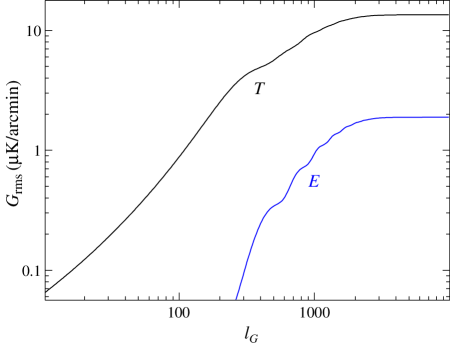
Instead let us exploit the fact that we have robust prior knowledge about the unlensed CMB spectrum. A handful of well determined cosmological parameters fixes its shape out through the damping tail where the small scale gradients pick up most of their contribution. Fig. 1 shows the unlensed rms gradient as a function of a step function low pass filter $W^{TT}_{l}$ out to $l=l_{G}$

$$(G_{{\rm rms}}^{T})^{2} \equiv \langle\nabla\tilde{T}_{G}(\hat{\bf n})\cdot\nabla\tilde{T}_{G}(\hat{\bf n})\rangle$$ (10)

$$= \int_{1}^{l_{G}}{ldl\over 2\pi}l^{2}\tilde{C}_{l}^{TT}\,.$$

Almost all of the gradient comes from $l\leq 2000$ due to diffusion damping of the acoustic peaks. On these scales, the lensing correction to the gradient is tiny for a typical cluster. This suggests that if we impose a sharp filter on the gradient to exclude higher multipoles, we lose very little signal and gain a clean separation between the lensed and unlensed structure. Such a filter is also desirable for large scale reconstruction to eliminate pairs of modes that violate the gradient approximation. Furthermore, it also reduces contamination from foregrounds and systematics that might appear as signal without a clean separation of scales between the two fields of the quadratic estimator.

Now let us make these considerations concrete and generalize them to the full set of temperature and polarization fields $X,Y\in T,E,B$. $E(\hat{\bf n})$ and $B(\hat{\bf n})$ are real valued fields that are related to the Stokes parameters as

$$Q(\hat{\bf n})+iU(\hat{\bf n})=-\int{d^{2}l\over(2\pi)^{2}}[E_{\bf l}+iB_{\bf l}]e^{2i\varphi_{{\bf l}}}e^{i{\bf l}\cdot\hat{\bf n}}\,,$$ (11)

where $\varphi_{{\bf l}}$ is the angle between ${\bf l}$ and the axis which defines Stokes $Q$. We shall assume that $B$ is absent in the unlensed CMB.

The angular space convergence estimators

$$\hat{\kappa}^{XY}(\hat{\bf n})=\int{d^{2}l\over(2\pi)^{2}}e^{i{\bf l}\cdot\hat{\bf n}}\hat{\kappa}^{XY}_{{\bf l}}\,,$$ (12)

are constructed from Fourier space estimators that are quadratic in the observed fields

$${\hat{\kappa}^{XY}_{{\bf l}}\over A_{l}^{XY}}=-\int{d^{2}\hat{\bf n}}e^{-i\hat{\bf n}\cdot{\bf l}}{\rm Re}\left\{\nabla\cdot[{\bf G}^{XY}(\hat{\bf n})L^{Y*}(\hat{\bf n})]\right\}\,.$$ (13)

The gradient field ${\bf G}^{XY}$ is built out of the lensed $X$ field as either a spin-0 or spin-2 field depending on the spin of $Y$

$${\bf G}^{XY}_{\bf l}=i{\bf l}\,W^{XY}_{l}{X_{\bf l}}\times\Big{\{}\begin{array}[]{lr}1\,,&Y=T\,,\\ e^{2i\varphi_{{\bf l}}}\,,&Y=E,B\,.\\ \end{array}$$ (14)

$L^{Y}$ represents the lensed fields

$$L^{Y}_{\bf l}=W^{Y}_{l}{Y_{\bf l}}\times\Big{\{}\begin{array}[]{lr}1\,,&Y=T\,,\\ e^{2i\varphi_{{\bf l}}}\,,&Y=E,B\,.\end{array}$$ (15)

For the polarization fields, they are the Stokes field $Q+iU$ filtered for the $E$ and $B$ components. The 2 gradient fields and 3 lensed fields produce 6 estimators from the temperature and polarization fields for consistency checks. In addition, replacement of the divergence in Eq. (13) with curl should leave estimators that are consistent with noise.

$A_{l}^{XY}$ is a normalization coefficient set to return unbiased estimators under the fully linearized approximation. For arbitrary filter functions, it is determined by noting that Hu and Okamoto (2002)

$$\langle X_{{\bf l}_{1}}Y_{{\bf l}_{2}}\rangle=2f^{XY}({\bf l}_{1},{\bf l}_{2})\kappa_{\bf l}\,,$$ (16)

where ${\bf l}={\bf l}_{1}+{\bf l}_{2}\neq 0$ and

$$f^{TT}({\bf l}_{1},{\bf l}_{2}) = \tilde{C}_{l_{1}}^{TT}({\bf l}\cdot{\bf l}_{1})+\tilde{C}_{l_{2}}^{TT}({\bf l}\cdot{\bf l}_{2})\,,$$

$$f^{TE}({\bf l}_{1},{\bf l}_{2}) = \tilde{C}_{l_{1}}^{TE}\cos 2\varphi_{{\bf l}_{1}{\bf l}_{2}}({\bf l}\cdot{\bf l}_{1})+\tilde{C}_{l_{2}}^{TE}({\bf l}\cdot{\bf l}_{2})\,,$$

$$f^{TB}({\bf l}_{1},{\bf l}_{2}) = \tilde{C}_{l_{1}}^{TE}\sin 2\varphi_{{\bf l}_{1}{\bf l}_{2}}({\bf l}\cdot{\bf l}_{1})\,,$$

$$f^{ET}({\bf l}_{1},{\bf l}_{2}) = f^{TE}({\bf l}_{2},{\bf l}_{1})\,,$$

$$f^{EE}({\bf l}_{1},{\bf l}_{2}) = [\tilde{C}_{l_{1}}^{EE}({\bf l}\cdot{\bf l}_{1})+\tilde{C}_{l_{2}}^{EE}({\bf l}\cdot{\bf l}_{2})]\cos 2\varphi_{{\bf l}_{1}{\bf l}_{2}}\,,$$

$$f^{EB}({\bf l}_{1},{\bf l}_{2}) = \tilde{C}_{l_{1}}^{EE}\sin 2\varphi_{{\bf l}_{1}{\bf l}_{2}}({\bf l}\cdot{\bf l}_{1})\,.$$ (17)

Here $\varphi_{{\bf l}_{1}{\bf l}_{2}}\equiv\varphi_{{\bf l}_{1}}-\varphi_{{\bf l}_{2}}$. The normalization is given in terms of these quantities and the filters as

$${1\over A_{l}^{XY}}={2\over l^{2}}\int{d^{2}l_{1}\over(2\pi)^{2}}({{\bf l}\cdot{\bf l}_{1}})W_{l_{1}}^{XY}W_{l_{2}}^{Y}c^{Y}({\bf l}_{1},{\bf l}_{2})f^{XY}({\bf l}_{1},{\bf l}_{2})\,,$$

where

$$c^{T}({\bf l}_{1},{\bf l}_{2}) = 1\,,$$

$$c^{E}({\bf l}_{1},{\bf l}_{2}) = \cos 2\varphi_{{\bf l}_{1}{\bf l}_{2}}\,,$$

$$c^{B}({\bf l}_{1},{\bf l}_{2}) = \sin 2\varphi_{{\bf l}_{1}{\bf l}_{2}}\,.$$ (18)

For the lensed field filter, we retain the choice of Hu (2001a); Hu and Okamoto (2002)

$$W^{Y}_{l}=(C_{l}^{YY}+N_{l}^{YY})^{-1}\,.$$ (19)

As described above, the first modification is that the gradient weights are set to zero above $l_{G}=2000$

$$W_{l}^{XY}=0\,,\qquad(l>l_{G})\,.$$ (20)

Fig. 1 shows that this is also a good choice for the $E$ field. For $l\leq l_{G}$, we retain the Wiener filter

$$W_{l}^{XY}=\tilde{C}_{l}^{XY}(C_{l}^{XX}+N_{l}^{XX})^{-1}\,,\quad(l\leq l_{G})\,,$$ (21)

for $Y\in T,E$ and

$$W_{l}^{XB}=\tilde{C}_{l}^{XE}(C_{l}^{XX}+N_{l}^{XX})^{-1}\,,\quad(l\leq l_{G})\,,$$ (22)

for $Y=B$.

Secondly, we distinguish between $TE$ and $ET$ estimators. With the gradient filter employing only $l<l_{G}$, the scale symmetry between the two fields is broken. It is then advantageous to separate the estimators. The $TE$ estimator uses $T$ for the gradient field and $E$ for the lensed field. If contamination from unpolarized cluster emission is strong then this estimator can be used to eliminate its effects. The $ET$ estimator uses $E$ for the gradient field and $T$ for the lensed field. This estimator places less demanding requirements on the experiments in that only the relatively large $E$ field of the acoustic peaks need be measured to high signal to noise. Indeed this measurement need not come from the same experiment that measures the cluster signal. Both estimators strongly reject contaminants from foregrounds and systematics. Only the background CMB will have $T$ and $E$ correlated and anticorrelated in the specific oscillatory pattern of the acoustic peaks. Unfortunately, the sample variance of these estimators is also higher given the imperfect correlation between the two fields.

On the other hand, the sample variance of the $EB$ estimator is reduced by the fact that $B$ modes are assumed absent in the unlensed fields Hu and Okamoto (2002); Hirata and Seljak (2003). In practice the noise of the actual estimator will depend on the $B$-modes contributed by foregrounds and other contaminants. Like the $ET$ estimator, cross correlation of the large scale $E$ gradients with the small scale $B$-modes should help reduce any bias arising from contaminants. Since the experimental requirements for $EB$ are similar to that of $TE$, $TB$, and $EE$ but yield better prospects for constraints, we focus on the $EB$, $ET$ and $TT$ estimators in the next section.

III Idealized Examples

To illustrate the performance of the estimators, let us take the idealization that all lenses are NFW Navarro et al. (1997) dark matter halos and the observed CMB fields have no contaminants aside from white detector noise. We will address more realistic cases in a future work Vale et al. (2007). The estimators should remain nearly unbiased since to pass through the reconstruction filters, a contaminant must be antisymmetric around the cluster center with an axis whose direction is correlated with the large scale gradients. In addition, contaminants will not appear in the 6 quadratic estimators, especially those involving cross correlation, in the same way. They can however contribute substantially to the noise and we will examine here the performance of the estimators as a function of detector noise as a proxy for other contaminants.

The NFW density profile is given by Navarro et al. (1997)

$$\rho(r)\propto{1\over r/r_{s}(1+r/r_{s})^{2}}\,,$$ (23)

where the normalization coefficient can be expressed in terms of the mass of the halo. We define the mass to be that enclosed at $r_{180}$ defined to be the radius which encloses the mass at an overdensity of 180 times the mean density

$$r_{180}=\left({3M\over 4\pi}{1\over{180\Omega_{m}\rho_{c}}}\right)^{1/3}\,,$$ (24)

where $\rho_{c}$ is the critical density today. Likewise, we define the concentration of the halo in terms of this radius

$$c_{180}={r_{180}\over r_{s}}\,.$$ (25)

The convergence profile for such a halo is Bartelmann (1996)

$$\kappa(\theta)={3\over 4\pi}{H_{0}D_{L}}{D_{LS}\over{D_{S}}}(1+z_{L}){MH_{0}\over\rho_{c}r_{s}^{2}}{g(\theta/\theta_{s})\over f({c_{180}})}\,,$$ (26)

where the projected scale radius $\theta_{s}=r_{s}/D_{L}$. $D$ is the comoving distance in a flat universe with subscripts “L” denoting the distance to the lens, “S” denoting distance to the source, and “LS” the distance between the lens and source. A primary advantage of the CMB is that the source is behind all clusters and at a well-determined distance $D_{S}=14.3$Gpc. The concentration factor is

$$f(c)=\ln(1+c)-{c\over 1+c}\,,$$ (27)

and the functional form of the profile is Bartelmann (1996)

$$g(x) = {1\over x^{2}-1}\left[1-{2\over\sqrt{x^{2}-1}}{\rm atan}\sqrt{{x-1\over x+1}}\right],\quad(x>1)$$ (28)

$$= {1\over x^{2}-1}\left[1-{2\over\sqrt{1-x^{2}}}{\rm atanh}\sqrt{{1-x\over 1+x}}\right],\quad(x<1)$$

$$= {1\over 3}\,,\quad(x=1)\,.$$

For illustrative purposes, we take

$$M_{14}\equiv{M\over 10^{14}h^{-1}M_{\odot}}=2\,,$$ (29)

$c_{180}=3.2$ and $z_{L}=0.7$. For these parameters $\theta_{s}=0.94^{\prime}$ and $\kappa(\theta_{s})=0.1$. Note the low value of the concentration reflects the low $\sigma_{8}$ fiducial cosmology and is determined by the scaling of Bullock et al. (2001). In a higher $\sigma_{8}$ cosmology, clusters at a fixed mass are more concentrated but correspondingly larger clusters are more abundant. Other numbers are typical of SZ selected clusters with upcoming surveys.

Figure 2: Temperature ($TT$) reconstruction in the absence of detector noise and other contaminants. From left to right, top to bottom the reconstructions are stacked with 1, 10, $10^{2}$, $10^{3}$ identical clusters of $M_{14}=M/10^{14}h^{-1}M_{\odot}=2$ and $z=0.7$. Shown here is a $35^{\prime}\times 35^{\prime}$ region around the cluster.

For the simulated reconstruction we consider a fiducial experiment with a $\theta_{\rm FWHM}=1^{\prime}$ beam and varying levels of noise on the sky

$$N_{l}^{TT} = \Delta_{T}^{2}B_{l}^{-2}\,,$$

$$N_{l}^{EE} = N_{l}^{BB}=\Delta_{P}^{2}B_{l}^{-2}\,.$$ (30)

where the beam factor is

$$B_{l}=e^{-l^{2}\theta_{\rm FWHM}^{2}/16\ln 2}$$ (31)

with $\theta_{\rm FWHM}$ in radians. It exponentiates the white detector noise on the beam deconvolved sky. We further assume that $\Delta_{P}=\sqrt{2}\Delta_{T}$. For this fiducial beam, a pixel scale of $\theta_{\rm pix}=0.2^{\prime}$ suffices. The field is chosen to be $512\times 512$ pixels $(100^{\prime}\times 100^{\prime})$.

We lens realizations of $\tilde{C}_{l}^{TT}$, $\tilde{C}_{l}^{EE}$ according to the full non-linear prescription of Eq. (1) with 6th order polynomial interpolation of the source image. This procedure allows strong lensing effects to appear at the center of the cluster. To this lensed image we add a realization of the noise power spectra above.

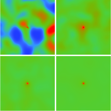
In Fig. 2, we show the reconstruction with $\Delta_{T}=0$ simulations of the $TT$-estimator for $N=1$, 10, $10^{2}$, and $10^{3}$ stacked clusters. In this detector noise free limit, there is a clear detection with only one cluster. It appears as a concentrated spike on top of a noisy but slowly varying background from chance correlations of the Gaussian random background field. The reconstructed single image lacks the azimuthal symmetry of the lens but symmetry is recovered by stacking images Maturi et al. (2005). This asymmetry comes from the fact that the deflections cannot be estimated in the direction orthogonal to the gradient. The estimator however is unbiased once many realizations of the gradient are stacked.

Figure 3: Recovered cluster-mass correlation function or stacked profile with 24000 detector noise free simulations. Bands represent the rms fluctuation per 1000 clusters in the sample. For $M_{14}=2$, the reconstruction has no detectable bias at the $1-2\%$ level within a few arcmin.

Stacking is equivalent to measuring the cluster-convergence correlation function

$$\xi_{c\kappa}(\theta)=\int{d\phi\over 2\pi}\langle\hat{\kappa}(\theta,\phi)\rangle\,,$$ (32)

where the coordinates are centered at the location of the cluster such that $\theta$ is the separation from the center and $\phi$ is the azimuthal angle around the cluster. The averaging is over the clusters in the sample. By defining the observable as the cluster-convergence correlation function, the estimator naturally generalizes to non-identical clusters and projected mass along the line of sight associated with the cluster. In practice, we evaluate the correlation function at discrete intervals in pixel units by interpolation on the stacked image. Neighboring bins out to several arcminutes are therefore highly correlated as can be seen directly in Fig. 2. This correlation is in fact useful for distinguishing the signal from noise.

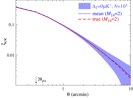
In Fig. 3, we show the recovered correlation function from $24000$ detector noise free realizations along with the scatter per 1000 clusters with $M_{14}=2$. We have smoothed both the lens and reconstruction with a $1.5$ pixel FWHM beam after the fact for comparison. The estimator has no detectable bias at the $\sim 1-2\%$ level in the well-measured regime within a few scale radii. At five times the fiducial mass or $M_{14}=10$, a low bias of $\sim 8-9\%$ develops for the fiducial gradient cut of $l_{G}=2000$. For these very rare clusters, the signal is large enough that a more aggressive $l_{G}=1000$ yields a bias free reconstruction with sufficient signal to noise. Alternately, the bias can be calibrated out with simulations.

Figure 4: Beam filtered correlation function from 12000 clusters. The reconstruction is low pass filtered at $l<l_{\rm beam}(=8095)$ to remove contributions below the beam scale. Shown for comparison are the filtered input lens of $M_{14}=2$ and a trial model of $M_{14}=2.6$ for comparison. With a noise level of $10\mu$K^′ the two cases are clearly distinguished.

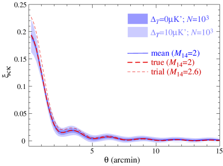
For cases with finite noise, we explicitly remove effects below the beam scale for numerical convenience. We low pass filter both the lens and the reconstruction with a step function at $l_{\rm beam}=\sqrt{8\ln 2}/\theta_{\rm FWHM}$. This also has the desirable effect of making the reconstruction less sensitive to potential contamination near the cluster center. The filtered correlation function is shown in Fig. 4 and remains unbiased and well-defined. It is equivalent to measuring the cross power spectrum at multipoles $l<l_{\rm beam}$. Fig. 4 also shows that with $\Delta_{T}=10\mu$K^′, $M_{14}=2$ and $2.6$ are significantly distinguished.

To quantify this sensitivity, we compute the covariance matrix of the correlation function from the simulations

$$C(\theta,\theta^{\prime})=\langle\hat{\xi}_{c\kappa}(\theta)\hat{\xi}_{c\kappa}(\theta^{\prime})\rangle-\xi_{c\kappa}(\theta)\xi_{c\kappa}(\theta^{\prime})\,,$$ (33)

where the discretization again is in bins of the pixel width. To estimate the significance with which two models can be separated, we evaluate $\Delta\chi^{2}$ between a test model $\xi_{c\kappa}^{\prime}(\theta)$ and the true model $\xi_{c\kappa}(\theta)$

$$\Delta\chi^{2}=\sum_{\theta,\theta^{\prime}}[\xi_{c\kappa}^{\prime}(\theta)-\xi_{c\kappa}(\theta)]{\bf C}^{-1}[\xi_{c\kappa}^{\prime}(\theta^{\prime})-\xi_{c\kappa}(\theta^{\prime})]\,,$$ (34)

summed out to $\theta=5^{\prime}$. Beyond a few scale radii of the cluster the correlation function is dominated by large scale structure.

Figure 5: Idealized mass sensitivity for $\theta_{\rm FWHM}=1^{\prime}$, $\theta\leq 5^{\prime}$. The fractional errors on the idealized NFW mass with 1000 clusters for the $TT$, $ET$ and $EB$ estimators. Unrelated mass along the line of sight will add noise to the estimates as will any emission from the cluster. No information from the reconstruction is used below the beam scale $l\geq l_{\rm beam}$.

In Tab. 1, we show the detection significance, the difference between the fiducial $M_{14}=2$ lens and zero with the covariance matrix evaluated at zero signal. We have scaled the significance per cluster by $\sqrt{N}$ for $N=10^{3}$. At a noise level of $10\mu$K^′, the significance or signal to noise is $\sqrt{\Delta\chi^{2}}\sim 0.4$ per cluster. Above this noise level, only $TT$ and $ET$ can provide significant detections. Although $TT$ has roughly three times the signal-to-noise, $ET$ can still provide a useful check against contamination and systematics for a first detection. Recall that the filter construction involves the oscillatory acoustic $TE$ correlation and strongly rejects spurious signals. At noise levels between $1-3\mu$K^′, the $EB$ estimator has both the signal-to-noise and the ability to reject contaminants to make it competitive with $TT$. Below $1\mu$K^′, the $EB$ estimator dominates.

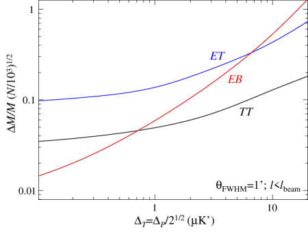
In Fig. 5 we plot the sensitivity to the cluster mass. Specifically we calculate the fractional change in mass that would generate a $\Delta\chi^{2}=1$ with $10^{3}$ clusters. The covariance is evaluated at the true model $M_{14}=2$ so as to include the sample variance of the unlensed gradients. The same features found for detection significance hold for mass sensitivity. For example at $10\mu$K^′, $TT$, $ET$, and $EB$ provide 13%, 43%, 53% mass estimates whereas at $1\mu$K^′ the numbers improve to 5%, 14%, 6%.

Finally, these sensitivities depend on the beam scale only weakly near the fiducial $\theta_{\rm FWHM}=1^{\prime}$ and $\Delta_{T}=1-10\mu$K^′ level. For example, at $3\mu$K^′, improving the beam to $0.5^{\prime}$ has negligible effect on the signal to noise. Enlarging the beam to $2^{\prime}$, degrades the $TT$ and $ET$ estimators by $\sim 30-40\%$ in mass sensitivity. Since the $EB$ estimator is noise dominated at the $1^{\prime}$ scale even without beam, it degrades negligibly.

Table 1: Detection significance $\sqrt{\Delta\chi^{2}}$ or S/N for $10^{3}$ clusters of $M_{14}=2$, $z=0.7$ and $\theta_{\rm FWHM}=1^{\prime}$.

Type	$3\mu$K′	$10\mu$K′	30$\mu$K′
$TT$	22.9	11.5	6.1
$ET$	8.0	3.5	1.4
$EB$	8.6	2.4	0.6

IV Discussion

We have developed mass estimators from 6 quadratic combinations of CMB temperature and polarization fields that retain their minimum variance characteristic for large scale structure and provide nearly unbiased reconstructions for rare clusters where lensing effects are moderate to strong. The key difference from previous work Hu (2001a); Hu and Okamoto (2002) is that the Wiener filtering for unlensed CMB gradients is augmented with a sharp filter that removes any gradients at $l_{G}>2000$ that are not part of the source fields from recombination.

This sharp filter should also help prevent false signals from cluster emission such as the thermal and kinetic Sunyaev-Zel’dovich effect, point source emission as well as other foregrounds. To even appear as excess noise, the contaminant at $\sim 1^{\prime}$ must have a component that is antisymmetric about the cluster center. To bias the measurement, the direction of the asymmetry must be correlated with both the polarized and unpolarized contamination at $\sim 10^{\prime}$ in the same way as the acoustic oscillations in the CMB. Note that projection effects from mass associated with the cluster should be considered part of the signal and can be calibrated by $N$-body simulations. True contaminants however can substantially increase the noise of the estimators. An evaluation of the efficacy of the filter in the presence of real world contaminants is beyond the scope of this paper but will be treated in future work Vale et al. (2007).

Here we have tested the estimators against idealized signal and noise: identical clusters lenses with NFW dark matter profiles in the presence of beam filtered white noise. At a noise level of $10\mu$K^′ and with a $1^{\prime}$ beam, the $TT$ estimator can provide a $\sim 10\sigma$ detection per $10^{3}$ clusters of $M\sim 2\times 10^{14}h^{-1}M_{\odot}$ or equivalently a $\sim 10\%$ average mass measurement. The $ET$ estimator, based on a separate measurement of $E$-polarization in the acoustic peaks and $T$ measurements around the cluster, can provide an important cross check on a first detection. Since the estimator filters for the $TE$ correlation and anticorrelation of the acoustic peaks it provides a strong discriminant against contamination and systematics at the price of a factor of $\sim 3$ in signal-to-noise. Ultimately with experiments that produce foreground free maps of the polarization to $<3\mu$K^′, the $EB$ estimator will return the best estimates, with the potential to ultimately provide $\sim 1\%$ measurements.

Acknowledgments We thank Tom Crawford, Gil Holder, Kendrick Smith, Scott Dodelson, and Jeremy Tinker for useful conversations. W.H. and S.D. were supported by the KICP under NSF PHY-0114422. W.H. was additionally supported by U.S. Deptartment of Energy contract DE-FG02-90ER-40560 and the David and Lucile Packard Foundation. C.V. was supported by the U.S. Department of Energy and by NASA grant NAG5-10842.

References

- Seljak and Zaldarriaga (2000) U. Seljak and M. Zaldarriaga, Astrophys. J. 538, 57 (2000), eprint astro-ph/9907254.
- Nagai et al. (2003) D. Nagai, A. V. Kravtsov, and A. Kosowsky, Astrophys. J. 587, 524 (2003), eprint astro-ph/0208308.
- Dodelson (2004) S. Dodelson, Phys. Rev. D 70, 023009 (2004), eprint astro-ph/0402314.
- Holder and Kosowsky (2004) G. P. Holder and A. Kosowsky, Astrophys. J. 616, 8 (2004), eprint astro-ph/0401519.
- Vale et al. (2004) C. Vale, A. Amblard, and M. White, New Astronomy 10, 1 (2004), eprint astro-ph/0402004.
- Maturi et al. (2005) M. Maturi, M. Bartelmann, M. Meneghetti, and L. Moscardini, Astron. Astrophys. 436, 37 (2005), eprint astro-ph/0408064.
- Lewis and King (2006) A. Lewis and L. King, Phys. Rev. D 73, 063006 (2006), eprint astro-ph/0512104.
- Hu (2001a) W. Hu, Astrophys. J Lett. 557, L79 (2001a), eprint astro-ph/0105424.
- Hu and Okamoto (2002) W. Hu and T. Okamoto, Astrophys. J. 574, 566 (2002), eprint astro-ph/0111606.
- Hirata and Seljak (2003) C. M. Hirata and U. Seljak, Phys. Rev. D67, 043001 (2003), eprint astro-ph/0209489.
- Guzik and Seljak (2001) J. Guzik and U. Seljak, Mon. Not. R. Astron. Soc. 321, 439 (2001).
- Johnston et al. (2005) D. E. Johnston et al. (2005), eprint astro-ph/0507467.
- Amblard et al. (2004) A. Amblard, C. Vale, and M. White, New Astronomy 9, 687 (2004), eprint astro-ph/0403075.
- Okamoto and Hu (2003) T. Okamoto and W. Hu, Phys. Rev. D 67, 083002 (2003), eprint astro-ph/0301031.
- Hu (2001b) W. Hu, Phys. Rev. D 64, 083005 (2001b), eprint astro-ph/0105117.
- Challinor and Chon (2002) A. Challinor and G. Chon, Phys. Rev. D66, 127301 (2002), eprint astro-ph/0301064.
- Zaldarriaga (2000) M. Zaldarriaga, Phys. Rev. D 62, 063510 (2000), eprint astro-ph/9910498.
- Challinor and Lewis (2005) A. Challinor and A. Lewis, Phys. Rev. D71, 103010 (2005), eprint astro-ph/0502425.
- Navarro et al. (1997) J. F. Navarro, C. S. Frenk, and S. D. M. White, Astrophys. J. 490, 493 (1997).
- Vale et al. (2007) C. Vale, S. De Deo, and W. Hu, in preparation (2007).
- Bartelmann (1996) M. Bartelmann, Astron. Astrophys. 313, 697 (1996), eprint astro-ph/9602053.
- Bullock et al. (2001) J. S. Bullock et al., Mon. Not. R. Astron. Soc. 321, 559 (2001).