Study on polarization of high-energy photons from the Crab pulsar

Abstract

We investigate polarization of high-energy emissions from the Crab pulsar in the frame work of the outer gap accelerator. The recent version of the outer gap, which extends from inside the null charge surface to the light cylinder, is used for examining the light curve, the spectrum and the polarization characteristics, simultaneously. The polarization position angle curve and the polarization degree are calculated to compare with the Crab optical data. We show that the outer gap model explains the general features of the observed light curve, the spectrum and the polarization by taking into account the emissions from inside of the null charge surface and from tertiary pairs, which were produced by the high-energy photons from the secondary pairs. For the Crab pulsar, the polarization position angle curve indicates that the viewing angle of the observer measured from the rotational axis is greater than $90^{\circ}$.

1 Introduction

Young pulsars such as the Crab pulsar are strong $\gamma$-ray sources. The EGRET instrument revealed that the light curve with double peaks in a period and the spectrum extending to above GeV are typical features of the high-energy emissions from the $\gamma$-ray pulsars. Although these data have constrained proposed models, the origin of the $\gamma$-ray emission is not yet conclusive. On important reason is that various models have successfully explained the features of the observed spectra and/or light curves. For example, the polar cap model (Daugherty & Harding 1996), the caustic model (Dyks et al. 2004) and the outer gap model (Cheng et al. 2000, hereafter CRZ00), all expect the main features of the observed light curve. So, we cannot discriminate the three different models using the light curve. Furthermore, both polar cap and outer gap models have explained the observed $\gamma$-ray spectrum (Daugherty & Harding 1996; Romani 1996).

Polarization measurement will play an important role to discriminate the various models, because it increases observed parameters, namely, polarization degree (p.d.) and position angle (p.a.) swing. So far, only the optical polarization data for the Crab pulsar is available (Kanbach et al. 2005) in high energy bands. For the Crab pulsar, the spectrum is continuously extending from optical to $\gamma$-ray bands. In addition, their pulse positions are considered so well that the optical emission mechanism is related to higher energy emission mechanisms. In the future, the next generation Compton telescope will probably be able to measure polarization characteristics in MeV bands. These data will be useful for discriminating the different models.

In this paper, we examine the optical polarization characteristics of the Crab pulsar with the light curve and the spectrum in frame works of the outer gap model. CRZ00 has calculated the synchrotron self-inverse Compton scattering process of the secondary pairs produced outside the outer gap and has explained the Crab spectrum from X-ray to $\gamma$-ray bands. In CRZ00, however, the outer-wing and the off-pulse emissions of the Crab pulsars cannot be reproduced, because the traditional outer gap geometry, which extends from the null charge surface of the Goldreich-Julian charge density to the light cylinder, is assumed. Furthermore, the spectrum in the optical band was not considered. In this paper, on these grounds, we modify the CRZ00 geometrical model into a more realistic model, following recent 2-D electrodynamical studies (Takata et al. 2004; Hirotani 2006), and calculate the light curve, the spectrum and the polarization characteristics of the Crab pulsar.

2 Calculation method

The outline of the outer gap model for the Crab pulsar is as follows. The charge particles are accelerated by the electric field parallel to the magnetic field lines in so called gap, where the charge density is different from the Goldreich-Julina charge density. The high energy particles accelerated in the gap emit the $\gamma$-ray photons (called primary photons) via the curvature radiation process. For the Crab pulsar, most of the primary photons escaping from the outer gap will convert into secondary pairs outside the gap, where the accelerating electric field vanishes, by colliding with synchrotron X-rays emitted by the secondary pairs. The secondary pairs emit optical - MeV photons via the synchrotron process and photons above MeV with the inverse Compton process. The high-energy photons emitted by the secondary pairs may convert into tertiary pairs at higher altitude by colliding with the soft X-rays from the stellar surface. The tertiary pairs emit the optical-UV photons via the synchrotron process. This secondary and tertiary photons appear as the observed radiations from the Crab pulsar

2.1 Outer gap

We consider the outer gap geometry that is extending from inside null charge surface to near the light cylinder (Takata et al 2004; Hirotani 2006). Because the Crab pulsar has a thin gap, we describe the accelerating electric field (Cheng et al. 1986) with

$$E_{||}(r)=\frac{\Omega B(r)f^{2}(r)R_{lc}^{2}}{cs(r)},$$ (1)

where $f(r)$ is the local gap thickness in units of the light radius, $R_{lc}=c/\Omega$, and $s(r)$ is the curvature radius of the magnetic field line. The typical fractional size of the outer gap is given by $f(R_{lc}/2)\sim 5.5B^{-4/7}P^{26/21}$ ($\sim 0.04$ for the Crab pulsar) and the local fractional size is estimated by $f(r)\sim f(R_{lc}/2)(2r/R_{lc})^{1.5}$ (Zhang & Cheng 1997).

The electric field described by equation (1) can be adopted for the acceleration beyond the null charge surface. Inside null charge surface, the electric field rapidly decreases because of the screening effects of the pairs. To simulate the accelerating electric field inside null charge surface, we assume the following field,

$$E_{||}(r)=E_{n}\frac{(r/r_{i})^{2}-1}{(r_{n}/r_{i})^{2}-1},~{}~{}r_{i}\leq r\leq r_{n},$$ (2)

where $E_{n}$ is the strength of the electric field at the null charge surface and $r_{n}$ and $r_{i}$ are the radial distances to the null charge surface and the inner boundary of the gap, respectively. The local Lorentz factor of the accelerated particles in the outer gap is described by $\Gamma_{e}(r)=[3s^{2}(r)E_{||}/2e]^{1/4}$ with assuming the force balance between the acceleration and the curvature radiation back reaction.

We assume that the outer gap extends around the whole polar cap. In the calculation, we constrain the boundaries of the axial distance and radial distance for the emission regions with $\rho_{\max}=0.9R_{lc}$ and $r=R_{lc}$, respectively.

2.2 Synchrotron radiation from the pairs

We calculate the synchrotron radiation at each radiating point following CRZ00. The photon spectrum of the synchrotron radiation is (CRZ00)

$$F_{syn}(E_{\gamma},r) = \frac{3^{1/2}e^{3}B(r)\sin\theta_{p}(r)}{mc^{2}hE_{\gamma}}$$ (3)

$$\times \int\left[\frac{dn_{e}(r)}{dE_{e}}\right]F(x)dE_{e}dV_{rad},$$

where $x=E_{\gamma}/E_{syn}$, $E_{syn}$ is the typical photon energy, $\theta_{p}$ is the pitch angle of the particle, $F(x)=x\int_{x}^{\infty}K_{5/3}(y)dy$, where $K_{5/3}$ is the modified Bessel function of order 5/3, $dn_{e}/dE_{e}\propto E_{e}^{-2}$ is the distribution of the pairs and $dV_{rad}$ is the volume element of the radiation region considered.

The pitch angle of the secondary pairs is estimated from $\sin\theta_{p}(R_{lc})\sim\lambda/s(R_{lc})$, where $\lambda$ is the mean free path of the pair-creation between the primary $\gamma$-rays and the non-thermal X-rays from the secondary pairs. For the Crab pulsar, the mean free path becomes $\lambda\sim(n_{X}\sigma_{\gamma\gamma})^{-1}\sim 10^{7}\mathrm{cm}$, where we used the typical number density $n_{X}\sim L_{X}(<E_{X}>)/\delta\Omega R_{lc}^{2}c<E_{X}>\sim 8\times 10^{17}~{}\mathrm{cm}^{-3}$, the luminosity $L_{X}\sim 10^{35}\mathrm{erg/s}$, the typical soft-photon energy for the pair-creation, $<E_{X}>\sim(2m_{e}c^{2})^{2}/10~{}\mathrm{GeV}\sim 100$ eV, and $\sigma_{\gamma\gamma}\sim\sigma_{T}/3$. Therefore the pitch angle of the secondary pairs at the light cylinder is estimated as $\sin\theta_{p}\sim\lambda/s(R_{lc})\sim 0.06$, and the local pitch angle is calculated from $\sin\theta_{p}(r)=\sin\theta_{p}(R_{lc})(r/R_{lc})^{1/2}$.

Some high-energy photons emitted by the inverse Compton process of the secondary pairs may convert into tertiary pairs at higher altitude by colliding with thermal X-ray photons from the star. In this paper, we assume that the maximum energy of and the local number density of the tertiary pairs are smaller than about $10\%$ of those of the secondary pairs. Because the pitch angle of the pairs increases with altitude, we use $\sin\theta_{p}=0.1$ for the pitch angle of the tertiary pairs. In fact, the results are not sensitive to the pitch angle of the tertiary pairs.

2.3 Stokes parameters

For a high Lorentz factor, we can anticipate that the emission direction of the particles coincides with the direction of the particle’s velocity. In the inertial observer frame, the particle motion may be described by

$$\mbox{\boldmath$n$}=\beta_{0}\cos\theta_{p}\mbox{\boldmath$b$}+\beta_{0}\sin\theta_{p}\mbox{\boldmath$b$}_{\perp}+\beta_{co}\mbox{\boldmath$e$}_{\phi},$$ (4)

where the first term in the right hand side represents the particle motion along the field line, for which we use the rotating dipole field, and $b$ is the unit vector of the magnetic field line. The second term in equation (4) represents gyration motion around the magnetic field line and $\mbox{\boldmath$b$}_{\perp}\equiv\cos\delta\phi\mbox{\boldmath$k$}+\sin\delta\phi\mbox{\boldmath$k$}\times\mbox{\boldmath$b$}$ is the unit vector perpendicular to the magnetic field line, where $\delta\phi$ refers the phase of gyration motion and $\mbox{\boldmath$k$}=(\mbox{\boldmath$b$}\cdot\nabla)\mbox{\boldmath$b$}/|(\mbox{\boldmath$b$}\cdot\nabla)\mbox{\boldmath$b$}|$ is the unit vector of the curvature of the magnetic field lines. The third term is co-rotation motion with the star, $\beta_{co}=\rho\Omega/c$. The emission direction of equation (4) is described in terms of the viewing angle measured from the rotational axis, $\xi=\cos^{-1}n_{z}$, and the rotation phase, $\Phi=-\Phi_{n}-\mbox{\boldmath$r$}\cdot\mbox{\boldmath$n$}$, where $n_{z}$ is the component of the emission direction parallel to the rotational axis, $\Phi_{n}$ is the azimuthal angle of the emission direction and $r$ is the emitting location in units of the light radius.

Because the particles distribute on the gyration phase $\delta\phi$, the emitted beam at each point must become cone like shape with opening angle $\theta_{p}(r)$. We calculate the radiations from the particles for all of the gyration phase $\delta\phi=2\pi i/n$ ($i=1,\cdots,n-1$).

We assume that the radiation at each point linearly polarizes with degree of $\Pi_{syn}=(p+1)/(p+7/3)$, where $p$ is the power law index of the particle distribution, and circular polarization is zero, that is, $V=0$ in terms of the Stokes parameters. The direction of the electric vector of the electro-magnetic wave toward the observer is parallel to the projected direction of the acceleration of the particle on the sky, that is, $\mbox{\boldmath$E$}_{em}\propto\mbox{\boldmath$a$}-(\mbox{\boldmath$n$}\cdot\mbox{\boldmath$a$})\mbox{\boldmath$n$}$ (Blaskiewicz et al. 1991). In the present case, the acceleration with equation (4) is approximately written by $\mbox{\boldmath$a$}\sim\beta_{0}\omega_{B}\sin\theta_{p}(-\sin\delta\phi\mbox{\boldmath$k$}+\cos\delta\phi\mbox{\boldmath$k$}\times\mbox{\boldmath$b$})$.

We define the position angle $\chi^{i}$ to be angle between the electric field $\mbox{\boldmath$E$}_{em}$ and the projected rotational axis on the sky. The Stokes parameters $Q^{i}$ and $U^{i}$ at each radiation is represented by $Q^{i}=\Pi_{syn}I^{i}\cos 2\chi^{i}$ and $U^{i}=\Pi_{syn}I^{i}\sin 2\chi^{i}$. After collecting the photons from the possible points for each rotation phase $\Phi$ and a viewing angle $\xi$, the expected p.d. and p.a. are, respectively, obtained from $P(\xi,\Phi)=\Pi_{syn}\sqrt{Q^{2}(\xi,\Phi)+U^{2}(\xi,\Phi)}/I(\xi,\Phi)$ and $\chi(\xi,\Phi)=0.5\mathrm{atan}\left[U(\xi,\Phi)/Q(\xi,\Phi)\right]$.

The inclination angle $\alpha$ and the viewing angles $\xi$ measured from the rotational axis are the model parameters. The radial distance $r_{i}$ of the inner boundary in equation (2) is also a model parameter, because the distance $r_{i}$ is determined by the current through the gap (Takata et al. 2004). Because the last-open line must be modified from the traditional magnetic surface, which is tangent to the light cylinder for the vacuum case, by the plasma effects (Romani 1996), the altitude of the upper surface of the outer gap, above which the pairs are created and emit the synchrotron photons, is used as a model parameter using a fractional polar angle $a=\theta_{u}/\theta_{lc}$, where $\theta_{u}$ is the polar angle of the footpoints of the magnetic field lines of the gap upper surface and $\theta_{lc}$ is the polar angle of the field lines which are tangent to the light cylinder for the vacuum case.

3 Results

Figure 1: Polarization characteristics for the traditional model (left column) and the present model (right column). The upper, middle and lower panels in each column show, respectively, the light curve, the position angle and the polarization degree for $\alpha=40^{\circ}$ and $a=0.93$.

Figure 1 compares the polarization characteristics at 1 eV predicted by the traditional (left column) and the present (right column) outer gap models. The traditional model considers the emissions from the secondary pairs with the outer gap starting from the null charge surface of the Goldreich-Julian charge density, $r_{i}=r_{n}$. The present model takes into account the emissions from inside null charge surface and the tertiary pairs. We assume the outer gap starts from the radial distance of 68% of the distance to null charge surface, $r_{i}=0.68r_{n}$. The model parameters are $\alpha=40^{\circ}$, $a=0.93$ and $\xi\sim 101^{\circ}$, where the viewing angle is chosen so that the predicted phase separation between the two peaks is consistent with the observed value $\delta\Phi\sim 0.4$ phase.

From the pulse profiles, we find that the traditional model can not produce the outer-wing and the off-pulse emissions. On the other hand, the present model produces the outer-wing and the off-pulse emissions with the emissions from inside of the null charge surface.

As seen in the polarization characteristics by the traditional model, we find that the secondary emissions beyond the null charge surface make the polarization characteristics such that the polarization degree takes a lower value at the bridge phase and a larger value near the peaks. In the synchrotron case, the cone like beam is radiated at each point, and an overlap of the radiations from the different particles on the gyration phase causes the depolarization. For the viewing angle $\xi\sim 101^{\circ}$, the radiations from all gyration phases contribute to the observed radiation at the bridge phase, because the line of sight passes through middle part of the emission regions. In such a case, the depolarization is strong, and as a result, the emerging radiation from the secondary pairs polarizes with a very low p.d. ($<10\%$). Near the peaks, the radiations from the some range of gyration phases are not observed because the line of sight passes through the edge of the emission regions at peaks. In such a case, the depolarization is weaker and the emerging radiation highly polarizes.

In the polarization angle swing in the present model, the large swings appear at the both peaks, and the difference of the position angle between the off-pulse and the bridge phases is about 90 degree. We can see the effects of the tertiary pairs on the polarization characteristics at the bridge phase. By comparing the p.d. at the bridge phase, we find that tertiary pairs produce the radiations with $\sim 10\%$ of the p.d. at the bridge phase.

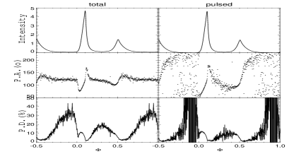
Figure 2: Optical polarization for the Crab pulsar. Left:Polarization characteristics for the total emissions. Right:Polarization characteristics of the emissions after subtraction of the DC level (Kanbach et al. 2005). The figures was transcribed from Dyks et al. (2004).

Figure 2 summarizes the Crab optical data. Left column and the right column show, respectively, the Crab optical data for the total emissions and for the emissions after subtraction of the DC level, which has the constant intensity at the level of 1.24% of the main pulse intensity. In the total emissions (left column), the impressive polarization feature is that the off-pulse and bridge phases have the fixed value of the p.a. These polarization features of the observation are not predicted by the present model. The present model are more consistent with the Crab optical data after the subtraction of the DC level. Especially, the model reproduces the most striking feature in the observed p.a. that the large swing at both peaks, and the observed low p.d. at bridge phase $\sim 10\%$. Also, the pattern of the p.d. are reproduced by the present model.

Figure 3 compares the model spectrum with the Crab data in optical-MeV bands. The model parameters are same with that in the right column in Figure 2. In this case, we assume that the pairs escape from the light cylinder with the Lorentz factor $\Gamma\sim 20$ due to the synchrotron cooling effect, which makes a spectral break around 10 eV in Figure 3. The model spectrum also explains the general features of the data. The outer gap model can explain the general features of the observed light curve, the spectrum and the polarization characteristics in optical band for the Crab pulsar, simultaneously.

It is worth to note that we can distinguish the two viewing angles mutually symmetric with respect to the rotational equator using the polarization swing. For such symmetric viewing angles, the light curves, the spectra and the p.d. curves are identical. However, the p.a. curves are mirror symmetry with respect to the rotational equator because of the difference directions of the projected magnetic field on the sky. The pattern of the position angle for the viewing angle smaller than $90^{\circ}$ swings to opposite directions from the Crab data at the both peaks. Therefore, the present model predicts that the viewing angle larger than $90^{\circ}$ are preferred for the Crab pulsar.

Figure 3: The optical-X ray spectrum for the Crab pulsar. The calculation is for $\alpha=40^{\circ}$, $a=0.93$, $r_{i}=0.68$ and $\xi\sim 101^{\circ}$. The X-ray data are taken from Kuiper et al. (2002) and reference therein, and the optical data from Sollerman et al. (2000).

4 Conclusions

We have considered the light curve, the spectrum and the polarization characteristics for the Crab pulsar predicted by the outer gap model which takes into account the emissions from inside the null charge surface and from the tertiary pairs. We have shown that the expected polarization characteristics are consistent with the Crab optical data after subtraction of the DC level. The outer gap model explains the spectrum, light curve and the polarization characteristics, simultaneously.

- [1] Blaskiewicz, M. et al. 1991, ApJ, 370, 643
- [2] Cheng, K.S., Ho, C. & Ruderman, M. 1986, ApJ, 300, 500
- [3] Cheng, K.S., Ruderman, M. & Zhang, L. 2000, ApJ, 537, 964
- [4] Daugherty, J.K. & Harding, A.K. 1996, ApJ, 458, 278
- [5] Dyks J., Harding A.K. & Rudak B. 2004, ApJ, 606, 1125
- [6] Hirotani, K. 2006, Mod. Phys. Lett. A 21, 1319
- [7] Kanbach, G. et al. 2005, AIP Conference Proceeding, 801, 306
- [8] Kuiper, L., et al. 2001, A&A, 378, 918
- [9] Romani R.W. 1996, ApJ, 470, 469
- [10] Sollerman, J. et al. 2000, ApJ, 537, 86
- [11] Takata, J., Shibata, S. & Hirotani K. 2004, MNRAS, 354, 1120
- [12] Takata, J. et al. 2006, MNRAS, 366, 1310
- [13] Zhang, L. & Cheng K.S. 1997, ApJ, 487. 370