The Environment of Local Ultraluminous Infrared Galaxies

Abstract

The spatial cluster-galaxy correlation amplitude, $B_{gc}$, is computed for a set of 76 $z<0.3$ ultraluminous infrared galaxies (ULIRGs) from the 1-Jy sample. The $B_{gc}$ parameter is used to quantify the richness of the environment within 0.5 Mpc of each ULIRG. We find that the environment of local ULIRGs is similar to that of the field with the possible exceptions of a few objects with environmental densities typical of clusters with Abell richness classes 0 and 1. No obvious trends are seen with redshift, optical spectral type, infrared luminosity, or infrared color ($f_{25}/f_{60}$). We compare these results with those of local AGNs and QSOs at various redshifts. The 1-Jy ULIRGs show a broader range of environments than local Seyferts, which are exclusively found in the field. The distribution of ULIRG $B_{gc}$-values overlaps considerably with that of local QSOs, consistent with the scenario where some QSOs go through a ultraluminous infrared phase. However, a rigorous statistical analysis of the data indicates that these two samples are not drawn from the same parent population. The $B_{gc}$ distribution of QSOs shows a distinct tail at high $B_{gc}$-values which is not apparent among the ULIRGs. This difference is consistent with the fact that some of the QSOs used for this comparison have bigger and more luminous hosts than the 1-Jy ULIRGs.

1 Introduction

Ultraluminous Infrared Galaxies (ULIRGs) are defined as galaxies with L_IR = L(8 $-$ 1000 $\mu$m) $\geq$ 10¹²L_⊙ (see reviews by Sanders & Mirabel 1996; Lonsdale, Farrah, & Smith 2006). This luminosity limit is roughly equivalent to the minimum bolometric luminosity of QSOs. At luminosities above 10¹²L_⊙, the space density of ULIRGs in the local universe is greater than that of optically selected quasars with similar bolometric luminosities by a factor of $\sim$ 1.5. Thus local ULIRGs represent the most common type of ultraluminous galaxy. Systematic optical and near-infrared imaging surveys have revealed that local ULIRGs are almost always undergoing major mergers (e.g., Surace & Sanders 1999; Surace, Sanders, & Evans 2001; Scoville et al. 2000; Veilleux et al. 2002, 2006). Most of the gas and star formation (and AGN) activity in these systems are concentrated well within the central kpc (e.g., Downes & Solomon 1998; Soifer et al. 2000, 2001). Ground-based optical and near-infrared spectroscopic studies of these objects have shown that at least 25% – 30% of them show genuine signs of AGN activity (e.g., Kim, Veilleux, & Sanders 1998; Veilleux, Kim, & Sanders 1997, 1999; Veilleux, Sanders, & Kim 1999). This fraction increases to $\sim$ 50% among the objects with log[$L_{\rm IR}/L_{\odot}$] $\gtrsim$ 12.3. These results are compatible with those from mid-infrared spectroscopic surveys (e.g., Genzel et al. 1998; Lutz et al. 1998; Lutz, Veilleux, & Genzel 1999; Rigopoulou et al. 1999; Tran et al 2001).

ULIRGs are relevant to a wide range of astronomical issues, including the role played by galactic mergers in forming some or all elliptical galaxies (Genzel et al. 2001; Veilleux et al. 2002), the efficiency of transport of gas into the central regions of such mergers and the subsequent triggering of circumnuclear star formation (e.g., Mihos & Hernquist 1996; Barnes 2004), the resulting heating and metal enrichment of the IGM by galactic winds (e.g. Rupke, Veilleux, & Sanders 2002, 2005ab; Veilleux, Cecil, & Bland-Hawthorn 2005; Martin 2005), the potential growth and fueling of supermassive black holes and the possible origin of quasars (Sanders et al. 1988). The discovery of $z=1-4$ submm sources with SCUBA (e.g., Smail et al. 1997; Hughes et al. 1998) suggests that ULIRGs are also relevant to the dominant source of radiant energy in the universe today. Indeed, integration of the light from the SCUBA population shows that it may account for most of the submm/far-infrared background, as a result of the strong cosmological evolution of these sources (e.g., Chapman et al. 2005). Thus, while the present-day ULIRGs provide a relatively small contribution to the total present background, their cousins at high $z$ are fundamentally important in this regard.

If ULIRGs are the predecessors of QSOs, one would expect ULIRGs and QSOs to live in similar environments. Surprisingly little has been published on the environments of local ULIRGs, in stark contrast to the abundant literature on the small- and large-scale environments of AGNs and QSOs (e.g., Yee, Green, & Stockman 1986; Yee & Green 1987; Ellingson et al. 1991; Hill & Lilly 1991; de Robertis et al. 1998; McLure & Dunlop 2001; Wold et al. 2000, 2001; Barr et al. 2003; Miller et al. 2003; Kauffmann et al. 2004; Söchting et al. 2004; Wake et al. 2004; Croom et al. 2005; Waskett et al. 2005; Serber, Bahcall, & Richards 2006) and the growing literature on the environments of $z\gtrsim 1$ ULIRGs (e.g., Blain et al. 2004; Farrah et al. 2004, 2006). To our knowledge, Tacconi et al. (2002) is the only published study that has attempted to quantify the environments of local ULIRGs. They correlated the positions of local ULIRGs with the catalogs of galaxy clusters and groups available in NED and found that none of them are located within a galaxy cluster. The lack of comprehensive imaging database at the time prevented them from carrying out a more quantitative clustering analysis of these objects.

The present paper remedies the situation by using the large imaging database of Veilleux et al. (2002) to quantify the environment of local ($\langle z\rangle\sim 0.15$) ULIRGs from the 1-Jy sample. We note that the spectroscopy portion of the Sloan Digital Sky Survey (SDSS) provides redshift information for only the bright tail of the galaxy luminosity function at $z\sim 0.15$, so a method that relies solely on the photometric measurements of the galaxies in the field surrounding the ULIRG must be used for the present analysis. The properties of the 1-Jy sample and imaging dataset are reviewed in §2. In §3, the procedure for deriving the environmental richness, $B_{gc}$, is outlined. Results for our sample are presented in §4. The findings of environmental studies for quasars and Seyferts are compared with our results in §5. Our conclusions are summarized in §6. We use $H_{0}$ = 50 km s^-1 Mpc^-1, $\Omega_{m}=1$, and $\Omega_{\lambda}$ = 0 throughout this paper. These values were selected to match those of previous studies and facilitate comparisons; they have no effect on our conclusions.

2 Sample

The IRAS 1-Jy sample of 118 ULIRGs identified by Kim & Sanders (1998) is the starting point of our investigation. The 1-Jy ULIRGs were selected to have high galactic latitude ($|b|$ $\geq$ 30^∘), 60-$\mu$m flux greater than 1 Jy, 60-$\mu$m flux greater than their 12-$\mu$m flux (to exclude infrared-bright stars), and ratios of 60-$\mu$m flux to 100-$\mu$m flux above $10^{-0.3}$ (to favor the detection of high-luminosity objects).

All 1-Jy ULIRGs were imaged at optical (R) and near-infrared (K^′) wavelengths using the U. of Hawaii 2.2-meter telescope. The present study uses only the R-band images since they have a larger field of view (FOV) and are deeper than the K^′-band images. The R filter at 6400 Å was a Kron-Cousins filter. Details of the observations and data reduction can be found in Kim, Veilleux, & Sanders (2002). The analysis of these data is presented in Veilleux et al. (2002). These data are part of comprehensive imaging and spectroscopic surveys which also include a large set of optical and near-infrared spectra of the nuclear sources (Veilleux et al. 1999ab and references therein), a growing set of spatially-resolved near-infrared spectra to study the gas and stellar kinematics of the hosts (Genzel et al. 2001; Tacconi et al. 2002; Dasyra et al. 2006a, 2006b), and mid-infrared spectra from the Infrared Space Observatory (ISO) and the Spitzer Space Telescope (SST; e.g., Genzel et al. 1998; Veilleux et al. 2006b, in prep.). This effort is called QUEST: Quasar / ULIRG Evolutionary Study.

Since the set of data presented in Kim et al. (2002) was compiled from observations made over the course of 14 years, a variety of CCDs were used and the FOV sizes and spatial resolutions are not uniform. For consistency, we limit the set of data in this paper to the images of the 76 objects taken under good photometric conditions with the TEK 2048 $\times$ 2048 CCD. Of these images, 32 (42%) were irrecoverably cropped during an earlier stage of data reduction and have a significantly reduced FOV size. The effects of the cropping on the results of our analysis are discussed in §4. Table 1 lists the objects in our sample along with the FOV size and several other properties of the sources.

3 Analysis

In this section we explain the methods that we used to quantify the environment richness around each ULIRG. First, we describe the algorithms used to find objects in the field and identify them as stars or galaxies. Next, we discuss the formalism applied to calculate the environment richness parameter, $B_{gc}$. The techniques used for our analysis have already been described in detail in Yee (1991), Ellingson et al. (1991), Yee & Lopez-Cruz (1999), and Gladders & Yee (2005); here we highlight the main steps.

3.1 Object Identification and Classification

Object identification was accomplished using the Picture Processing Package (PPP) developed by one of us (Yee 1991). This program systematically examines each pixel in the image and determines whether it has the potential to be part of an object: a star, a galaxy, a cosmic ray, or an artifact of the CCD. After running through a series of tests, the PPP object finding program identifies and catalogs the location and peak brightness of objects in the image. The algorithms used here are modified versions of that used by Kron (1980), which depend on searching for local maxima. They have been shown to be robust for object identification in sparse to moderately crowded fields (Yee 1991). The 1-Jy sample selection criterion $|b|\geq 30^{\circ}$ avoids extremely crowded fields (and reduces the effects of dust extinction on the galaxy counts), which could lead to object misclassification and erroneous environment richness measurements. We therefore find that this object finding routine is perfectly adequate for all ULIRGs in our sample

To address the problem of bad pixels or cosmic rays, objects were thrown out automatically if a given pixel was five times brighter than those immediately surrounding it. This did not always work well because bright bad pixels are sometimes surrounded by other bad pixels. So, some misidentified objects were also identified by eye and removed by hand.

The next step was to run an aperture photometry algorithm on the identified objects in each image to determine whether these objects are stars or galaxies. For each object, a growth curve was calculated using a series of circular apertures centered on the intensity centroid of the object. A reference-star growth curve was created for each quadrant of the CCD frame by averaging the growth curves of bright, isolated, and unsaturated stars within each quadrant. The growth curves of the other objects were then compared with the reference-star growth curve using the classification parameter $C_{2}$ defined by Yee (1991). In essence, $C_{2}$ computes the average difference per aperture between the growth curves of the objects and the growth curve of the reference star after they have been scaled to match at the center and effectively compares the ratio between the fluxes in the center and the outer part of an object with that of the reference star. This method has been thoroughly tested by Yee (1991); readers interested in knowing more about this classification scheme should refer to this paper for detail.

3.2 Environment Richness Parameter

We use the parameter $B_{gc}$ to quantify the richness of the environment of ULIRGs. $B_{gc}$ is the amplitude of the galaxy-galaxy correlation function calculated for each object of interest individually. It was first used by Longair & Seldner (1979) to measure the environment of radio galaxies using galaxy counts, and subsequently adopted in most studies of the environments of quasars and other active galaxies (e.g., Yee & Green 1984; Ellingson et al. 1991; de Robertis et al. 1998; McLure & Dunlop 2001; Wold et al. 2000, 2001; Barr et al. 2003; Waskett et al. 2005), and also used as a quantitative measurement of galaxy cluster richness (e.g., Andersen & Owen, 1994; Yee & López-Cruz 1999). Yee & Lopez-Cruz (1999) have demonstrated the robustness of the $B_{gc}$ parameter when galaxies are counted to different radii and to different depth. Furthermore, measurements of the environmental richness based on the photometrically-derived $B_{gc}$-values have been shown to be entirely consistent with measurements based on spectroscopic data. This was demonstrated by Yee & Ellingson (2003), who used the data from the Canadian Network for Observational Cosmology Cluster Redshift Survey (CNOC1) to compare $B_{gc}$-values derived from (1) photometric data with background subtraction, and (2) from properly weighted spectroscopy data to account for incompleteness. We describe briefly the procedure for deriving $B_{gc}$ below.

In order to determine the richness of the environment around a ULIRG, we need to count the number of galaxies within a spherical volume with radius, $r$, from the ULIRG of interest. However, we necessarily must begin with a two-dimensional image, which is a projection of this volume onto the sky plane. The number of galaxies in a solid angle $d\Omega$, at an angular distance $\theta$ from the object of interest is given by (Seldner & Peebles 1978)

$$N(\theta)d\Omega=N_{g}[1+\omega(\theta)]d\Omega,$$ (1)

where $N_{g}$ is the average surface density of galaxies and $w(\theta)$, the angular correlation function, can be expressed approximately as a power law,

$$w(\theta)=A_{gc}\theta^{1-\gamma}.$$ (2)

$A_{gc}$ is a measure of the average enhancement of galaxies in angular area, and $\gamma\approx 1.77$ empirically. Integrating equation (2) within a circle with radius $\theta$ yields

$$A_{gc}=\frac{N_{tot}-N_{bgc}}{N_{bgc}}\frac{(3-\gamma)}{2}\theta^{\gamma-1},$$ (3)

where $N_{tot}$ and $N_{bgc}$ are the the total numbers of galaxies and background galaxies, respectively, within an angular radius of $\theta$.

Next, the two-dimensional parameters must be translated into three dimensions. The angular correlation function $w(\theta)$ is translated into the spatial correlation function, $\xi(r)$, which describes the number of galaxies in volume element $dV$ at distance $r$ from the object of interest. It can be shown that $\xi(r)=B_{gc}r^{-\gamma}$, where $\gamma$ has the same value as in equation (3) and $B_{gc}$ is the spatial correlation amplitude, a measure of the richness of the environment around the galaxy. Longair & Seldner (1979) have shown that

$$B_{gc}=\frac{A_{gc}n_{bg}(m)D^{\gamma-3}}{I_{\gamma}\Psi(m,z)}.$$ (4)

The constant I_γ is an integration constant which depends on $\gamma$ (Groth & Peebles 1977). $n_{bg}(m)$ is the expected count per unit angular area of background galaxies brighter than apparent magnitude $m$, $\Psi(m,z)$ is the normalized integrated luminosity function of galaxies to apparent magnitude $m$, at redshift $z$ of the cluster, and $D$ is the angular diameter distance to the ULIRG at redshift $z$. For our calculations, we used $\gamma$ = 1.77, $I_{\gamma}$ = 3.78, and the cosmological parameters H₀ = 50 km s^-1Mpc^-1, $\Omega_{m}$ = 1, and $\Omega_{\lambda}$ = 0 to match those of previous papers. For $\Psi$ and $n_{bg}(m)$, we use the luminosity function and background counts derived from the Red-Sequence Cluster Survey (RCS; e.g., Gladders & Yee 2005).

The uncertainty on B_gc is computed using the formula

$$\frac{\Delta B_{gc}}{B_{gc}}=\frac{(N_{net}+1.3^{2}N_{bg})^{\text@frac{1}{2}}}{N_{net}}$$ (5)

where $N_{net}$ is the net counts of galaxies over the background counts, $N_{bg}$. This is a conservatively large error estimate as it includes the expected counting statistics in $N_{net}$ and the expected dispersion in background counts. The factor 1.3² is included to account approximately for the additional fluctuation from the clustered (and hence non-Poissonian) nature of the background counts (discussed in detail in Yee, Green, & Stockman 1986). We follow the prescription of Yee & López-Cruz (1999) and integrate the luminosity function from approximately $M_{R}=-25$ to $M^{*}_{R}+2$ (where $M^{*}_{R}\approx-22.3$ for our cosmology) to calculate the galaxy counts. This corresponds roughly to R = 15 – 20 for the galaxies in our sample ($\langle z\rangle\approx 0.15$). This range of integration was found by Yee & López-Cruz (1999) to reduce the sensitivity to small intrinsic variation of $M^{*}$ and variations in the faint-end slopes of the cluster luminosity function. The $B_{gc}$ parameter is computed over a radius $r=500$ kpc, either directly from the data when FOV $\geq$ 1 Mpc or extrapolated to this radius when FOV $<$ 1 Mpc. This radius is selected to match that of previous studies. The $B_{gc}$ parameter is not sensitive to this radius (Yee & Lopez-Cruz 1999; see also §4).

4 Results

The spatial correlation amplitude parameter, B_gc, was computed for each of the 76 ULIRGs in our sample. The B_gc-values and associated 1-$\sigma$ uncertainties are listed for each object in Table 1. The average (median) value of $B_{gc}$ and 1-$\sigma$ scatter around the mean for our sample of 76 ULIRGs is $\langle B_{gc}\rangle=35\pm 198$ Mpc^1.77 ($-3$ Mpc^1.77). For comparison, the $B_{gc}$-values of field galaxies and clusters of Abell richness class (ARC) 0-4 are $\sim$ 67.5, 600 $\pm$ 200, 1000 $\pm$ 200, 1400 $\pm$ 200, 1800 $\pm$ 200, and 2200 $\pm$ 200 Mpc^1.77 , respectively (the field $B_{gc}$-value is from Davis & Peebles 1983; the values for ARC 0-4 are from Yee & López-Cruz 1999). The average clustering around the local ULIRGs therefore corresponds to an environment similar to the field. A large scatter is seen in our data: although most objects are consistent with no galaxy enhancement, a few objects apparently lie in clusters of Abell classes 0 and 1.

Before discussing the results any further, it is important to verify that our analysis of the cropped (FOV $<$ 1 Mpc) images does not introduce any bias when compared with the results from the uncropped (FOV $\geq$ 1 Mpc) images. The average (median) $B_{gc}$-value for the 44 objects with uncropped images is 4 $\pm$ 121 Mpc^1.77 ($-$5 Mpc^1.77); i.e. slightly smaller than the values found for the entire sample. Statistical tests give mixed results regarding the significance of this discrepancy (Table 2). The results from a two-sided K-S (Kolmogorow-Smirnov) test, a Wilcoxon matched-pairs signed-ranks test, and a Student’s t-test on the means of the distributions suggest that the distribution of $B_{gc}$-values for the uncropped images is not significantly different from the distribution of $B_{gc}$-values as a whole, while the results from a F-test on the standard deviations of the distributions suggest a significant difference.

We have examined the distributions of $B_{gc}$-values for cropped and uncropped images as a function of Galactic latitudes and longitudes. Assuming that the $B_{gc}$-values are unaffected by stellar contaminants from our Galaxy, there should be no trend with Galactic latitude or longitude. Indeed, the distributions of $B_{gc}$-values with latitude and longitude are consistent with being random. Our data therefore confirm the results of Yee & López-Cruz (1999), who found that changing the counting radius by a factor of two, both increasing to 1 Mpc and decreasing to 0.25 Mpc, did not alter the $B_{gc}$-values significantly. However, given the mixed results from the statistical tests, we track the cropped and uncropped data using different symbols in the various figures of this paper. We have verified that none of the results discussed below are affected if the counting radius is chosen to be 0.25 Mpc or 1 Mpc rather than 0.50 Mpc, although quantization errors becomes noticeable when the counting radius is 0.25 Mpc due to poorer number statistics. A counting radius of 0.5 Mpc is adopted in the rest of this paper to match that of previous studies.

Next, we explore the possibility of a dependence of the environment richness on ULIRG properties. The first parameter we examine is the infrared luminosity (Fig. 1). Statistical tests indicate that no trend is present between $B_{gc}$ and $L_{IR}$. This is true for both the uncropped data and the entire sample. The same result is found when we examine the environment richness as a function of redshift (Fig. 2). Here, however, the redshift range covered by our ULIRGs is very narrow ($z$ = 0.1 – 0.22, if we exclude four objects in the sample), so this statement is not statistically very significant. Comparisons with the results of Blain et al. (2004) and Farrah et al. (2004, 2006) suggest that the environment of high-$z$ ULIRGs is richer than that of local ULIRGs. We return to this point in §5.

In Figure 2, we also distinguish between optical spectral types. We separate our sample into Seyfert 1s, Seyfert 2s, LINERs, and HII region-like galaxies based on the optical classification of Veilleux et al. (1999a). No obvious trends are observed with spectral type, but the subdivision of our sample into four subsets necessarily leads to poorer statistics. In Figure 3, we plot $B_{gc}$ as a function of log($f_{25}/f_{60}$), another clear indicator of AGN activity [objects with log($f_{25}/f_{60}$) $>$ –0.7 have “warm”, AGN-like IRAS colors]. The lack of trends in this figure and Figure 2 indicates that the nature of the dominant energy source in local ULIRGs (starburst or AGN) is not influenced by the environment. This result is consistent with the ULIRG – QSO evolutionary scenario of Sanders et al. (1988), where the nature of the dominant energy source varies with merger phase (starburst in early phases and QSO in late phases) but is independent of the environment (as long as the dispersion in velocity of the galaxies within the cluster is not too large to prevent mergers altogether).

5 Comparison with AGN Samples

In this section we compare our results with those from published environmental studies of AGNs and QSOs. Table 2 summarizes the statistical results of these comparisons and Figures 4 – 9 display the $B_{gc}$-values from the various samples. Unless otherwise noted in the text below, all data sets use the same cosmology.

5.1 Local Seyferts

First, we compare our results with those derived on nearby AGNs. De Robertis et al. (1998) studied the environments of nearby ($z<0.05$) Seyfert galaxies using the exact same procedure as the one we use here, so we can directly compare their results with ours. For the 27 galaxies with z $>$ 0.0045, de Robertis et al. (1998) find $\langle B_{gc}\rangle=40\pm 63$ Mpc^1.77 (median of 27 Mpc^1.77), consistent with the environment of field galaxies. Recent studies based on the SDSS database confirm this result (e.g., Miller et al. 2003; Wake et al. 2004). The average environment of local ULIRGs is therefore not dissimilar to that of local Seyferts. However, as indicated in Table 2, virtually all statistical tests except perhaps the t-test on the means indicate that the two $B_{gc}$ distributions are not drawn from the same parent population. Figures 4 and 5 show why that is the case: The distribution of $B_{gc}$-values among ULIRGs is distinctly broader than that of the Seyferts. This slight difference is also seen in Figure 6, where we display the distribution of local Seyferts and local ULIRGs as a function of Abell richness classes.

As discussed in §4, Seyfert-like ULIRGs do not reside in distinctly poorer or richer environments than non-Seyfert ULIRGs, so the broader scatter in ULIRG environments cannot be attributed to the broad range of AGN activity level within the ULIRG population. We note that typical error bars for the de Robertis et al. (1998) sample is $\sim$ 100 Mpc^1.77, while it is $\sim$ 150 Mpc^1.77 for the ULIRG sample. (The difference is due to the redshift difference between the samples – the ULIRG data requires counting to a fainter magnitude, which introduces larger uncertainties from background counts.) But the full ULIRG sample distribution is about 3 times broader than the Seyfert distribution – so, the broader distribution of the ULIRG sample cannot be fully explained by the larger error bars.

5.2 Local QSOs

Next, we compare our results with those derived on the nearby ($z\approx 0.2$) QSOs by Yee & Green (1984) and McLure & Dunlop (2001). The measurements of Yee & Green (1984) can be directly compared with our ULIRG results since their results were derived using the same method and parameters as that of the present study. McLure & Dunlop also apply the same formalism to calculate $B_{gc}$. However, they use a different analysis package to identify and classify the objects in the field and carry out the photometry. Their use of HST WFPC2 data also limits their survey area to only $\sim$ 200 kpc around the QSOs, smaller than even our cropped data. These possible caveats should be kept in mind when comparing their results with ours.

Yee & Green (1984) get $\langle B_{gc}\rangle=157\pm 208$ and a median of 134 Mpc^1.77 for 34 QSOs from the Palomar-Green sample (Schmidt & Green 1983), while McLure & Dunlop (2001) derive an average (median) $B_{gc}$ of 365 $\pm$ 404 Mpc^1.77 (241 Mpc^1.77) for a set of 44 radio-quiet and radio-loud QSOs and radio galaxies. If we limit our discussion to the QSOs in McLure & Dunlop sample (21 radio-quiet QSOs and 13 radio-loud QSOs), the average (median) $B_{gc}$ becomes 304 $\pm$ 350 Mpc^1.77 (218 Mpc^1.77). The average environment of the QSOs in both studies is therefore slightly richer than that of local ULIRGs. The $B_{gc}$ distributions of the two sets of local QSOs (particularly that of the McLure & Dunlop sample; see Fig. 5) show a distinct tail at high $B_{gc}$-values which is not apparent in the ULIRG distribution.

A quantitative analysis generally confirms that the $B_{gc}$ distributions of Yee & Green and $B_{gc}$ distributions for the radio-quiet and radio-loud QSOs from McLure & Dunlop are statistically different from that of the local ULIRGs (Table 2). However, note that the Wilcoxon test suggests that the difference is barely significant. Indeed, Figures 5, 7, and 8 show that there is considerable overlap between the B_gc distributions of 1-Jy ULIRGs and low-$z$ QSOs, particularly the PG QSOs. This result is consistent with the idea that some, but perhaps not all, of these QSOs may have formed through a IR-luminous phase like that observed at low redshift in the 1-Jy ULIRGs. A more physically meaningful test of this scenario would be to compare the environment of local QSOs with the environment of $z\gtrsim 0.5$ ULIRGs to take into account the finite duration of the ULIRG – QSO evolutionary sequence. The recent environmental studies of distant ULIRGs by Blain et al. (2004) and Farrah et al. (2004, 2006) indeed point to slightly richer environments, which more strongly resemble the environments of the QSOs from McLure & Dunlop.

A posteriori, the distinct high-$B_{gc}$ tail in the distribution of the QSOs of McLure & Dunlop (2001) is not unexpected given the host properties of these particular QSOs: $\sim$ 4-5 times larger host sizes and luminosities relative to the 1-Jy ULIRGs (Dunlop et al. 2003; Veilleux et al. 2002, 2006). More luminous hosts live in richer environments on average than hosts of lower luminosity. As pointed out by Veilleux et al. (2006) and Dasyra et al. (2006c), the hosts of the QSOs from the Palomar-Green sample (these QSOS are less radio and X-ray luminous than the QSOs of McLure & Dunlop 2001) are a better match in host size and luminosity to the local ULIRGs. This may explain the generally better (although not perfect) agreement between the environments of PG QSOs and 1-Jy ULIRGs.

5.3 Intermediate-Redshift QSOs

For the sake of completeness, we display in Figures 5, 6, and 9 the results from our study of local ULIRGs alongside the results presented by Ellingson et al. (1991), Wold et al. (2001), and Barr et al. (2003) for 63 radio-quiet and radio-loud QSOs at 0.3 $<z<0.6$, 20 radio-quiet QSOs at 0.5 $\leq z\leq 0.8$, and 20 radio-loud QSOs at 0.6 $<z<$ 1.1, respectively. All three groups use the same basic method outlined in §3 to calculate the spatial correlation amplitude, and all groups assume the same value for H₀. However, Ellingson et al. (1991) assume $q_{0}$ = 0.02 instead of 0.5 ($\Omega_{m}$ = 0.04 instead of 1, if $\Omega_{\lambda}$ = 0). There is no simple way to scale the $B_{gc}$-values for different cosmological models (other than $H_{0}$) since its computation is rather complicated (§3), so Figures 5, 6, and 9 show the $B_{gc}$-values corrected for the different $H_{0}$ but not the different $\Omega_{m}$. Once again, we see considerable overlap between the various distributions, but the statistical analysis formally rules out that they come from the same parent population (Table 2). The amount of overlap in $B_{gc}$-values is quite remarkable given the difference in redshifts between the various samples. These results further support a connection between ULIRGs and some QSOs.

6 CONCLUSIONS

We have derived the spatial cluster-galaxy correlation amplitude, $B_{gc}$, for 76 $z<0.3$ ULIRGs from the 1-Jy sample and compared our results with those in the literature on $z<0.05$ AGNs, $z\approx 0.2$ QSOs, and $0.3\lesssim z\lesssim 1$ QSOs. The main results are as follows:

1. Local ULIRGs live in environments which are similar on average to that of field galaxies. However, there are a few exceptions: some objects apparently lie in clusters of Abell classes 0 and 1.

2. The infrared luminosity, optical spectral type, and IRAS 25-to-60 $\mu$m flux ratios of ULIRGs show no dependence with environment.

3. The ULIRG environment does not vary systematically over the redshift range covered by our sample (mostly 0.1 $<z<$ 0.22).

4. There is a lot of overlap between the $B_{gc}$ distribution of local ULIRGs and those of local Seyferts, local QSOs, and intermediate-$z$ QSOs. However, quantitative statistical comparisons show that the various $B_{gc}$ distributions are not drawn from the same parent population. The average environment of ULIRGs appears to be intermediate between that of local Seyferts and local QSOs. Local ULIRGs show a broader range of environments than local Seyferts, which are exclusively found in the field. The $B_{gc}$ distribution of QSOs show a distinct tail at high values which is not seen among local ULIRGs. This slight environmental discrepancy between local QSOs and ULIRGs is not unexpected: recent morphological studies have found that some of the more radio and X-ray luminous local QSOs used in this comparison have more luminous and massive hosts than local ULIRGs. A better match in host and environmental properties is seen when the comparison is made with the PG QSOs.

5. Overall, the results of this study suggest that ULIRGs can be a phase in the lives of all types of AGNs and QSOs, but not all moderate-luminosity QSOs may have gone through a ULIRG phase. Published studies of the environments of more distant ULIRGs, perhaps the actual predecessors of the local QSOs we see today, provide further support for an evolutionary connection between ULIRGs and QSOs.

Table 1: Galaxies Properties

Name	$l$	$b$	$z$	log(${L_{IR}}\over{L_{\odot}}$)	ST	log(${{f_{25}}\over{f_{60}}}$)	Bgc	1-$\sigma$	Field
(1)	(2)	(3)	(4)	(5)	(6)	(7)	(8)	(9)	(10)
F00091$-$0738	95.6	$-$68.1	0.118	12.19	HII	$-$1.08	$-$80	97	1240
F00188$-$0856	100.5	$-$70.2	0.128	12.33	L	$-$0.85	$-$26	103	1330
F00397$-$1312	113.9	$-$75.6	0.261	12.90	HII	$-$0.74	25	137	2220
F00456$-$2904	326.4	$-$88.2	0.110	12.12	HII	$-$1.27	$-$34	94	1220
F00482$-$2721	49.4	$-$89.8	0.129	12.00	L	$-$0.80	45	111	1390
F01004$-$2237	152.1	$-$84.6	0.118	12.24	HII	$-$0.54	34	103	1290
F01166$-$0844	143.6	$-$70.2	0.118	12.03	HII	$-$1.01	70	109	1240
F01199$-$2307	183.3	$-$81.8	0.156	12.26	HII	$-$1.00	$-$26	112	1550
F01298$-$0744	151.1	$-$68.1	0.136	12.27	HII	$-$1.11	34	112	1390
F01355$-$1814	174.9	$-$75.9	0.192	12.39	HII	$-$1.07	$-$61	121	720
F01494$-$1845	184.3	$-$73.6	0.158	12.23	$-$	$-$0.93	$-$99	113	1620
F01569$-$2939	225.6	$-$74.9	0.141	12.15	HII	$-$1.09	$-$118	108	1430
F02411$+$0353	168.2	$-$48.6	0.144	12.19	$-$	$-$0.79	24	113	1450
F02480$-$3745	243.1	$-$63.0	0.165	12.23	$-$	$-$1.06	$-$70	114	1680
F03209$-$0806	192.0	$-$49.3	0.166	12.19	HII	$-$0.89	$-$71	115	1620
F03250$+$1606	168.7	$-$32.4	0.129	12.06	L	$-$0.96	$-$137	103	1330
Z03521$+$0028	188.4	$-$38.0	0.152	12.45	L	$-$1.10	$-$203	111	1520
F04074$-$2801	225.9	$-$46.4	0.153	12.14	L	$-$1.28	121	130	1520
F04103$-$2838	226.9	$-$45.9	0.118	12.15	L	$-$0.53	31	103	1240
F04313$-$1649	213.6	$-$37.8	0.268	12.55	$-$	$-$1.16	$-$17	135	2260
F05020$-$2941	231.5	$-$35.1	0.154	12.28	L	$-$1.29	301	153	1530
F05024$-$1941	220.1	$-$32.0	0.192	12.43	S2	$-$0.88	$-$25	121	1800
F05156$-$3024	233.2	$-$32.4	0.171	12.20	S2	$-$1.06	$-$3	116	1660
F08201$+$2801	195.3	$+$31.3	0.168	12.23	HII	$-$0.89	$-$173	123	650
F08474$+$1813	208.7	$+$34.1	0.145	12.13	$-$	$-$0.83	$-$36	181	580
F08591$+$5248	165.4	$+$41.0	0.158	12.14	$-$	$-$0.80	65	143	620
F09039$+$0503	225.0	$+$32.1	0.125	12.07	L	$-$1.09	$-$96	120	520
F09539$+$0857	228.5	$+$44.8	0.129	12.03	L	$-$0.98	$-$100	121	530
F10035$+$2740	202.7	$+$53.5	0.165	12.22	$-$	$-$0.83	414	198	650
F10091$+$4704	169.9	$+$53.2	0.246	12.67	L	$-$1.17	678	319	860
F10190$+$1322	227.2	$+$52.4	0.077	12.00	HII	$-$0.94	277	140	860
F10485$-$1447	264.6	$+$38.7	0.133	12.17	L	$-$0.84	$-$45	119	550
F10594$+$3818	180.5	$+$64.7	0.158	12.24	HII	$-$0.93	$-$11	125	620
F11028$+$3130	196.5	$+$66.6	0.199	12.32	L	$-$1.05	2	131	740
F11180$+$1623	235.9	$+$66.3	0.166	12.24	L	$-$0.80	119	156	650
F11223$-$1244	272.6	$+$44.7	0.199	12.59	S2	$-$0.98	35	136	740
F11387$+$4116	164.6	$+$70.0	0.149	12.18	HII	$-$0.86	180	160	600
Z11598$-$0112	278.6	$+$59.0	0.151	12.43	S1	$-$0.80	$-$21	111	1510
F12032$+$1707	254.8	$+$75.3	0.217	12.57	L	$-$0.74	$-$194	127	1970
F12127$-$1412	283.4	$+$62.0	0.133	12.10	L	$-$0.81	$-$121	117	550
F12265$+$0219	290.8	$+$62.4	0.159	12.73	S1	$-$0.36	$-$6	149	1570
F12359$-$0725	295.7	$+$63.4	0.138	12.11	L	$-$0.95	192	163	560
F12447$+$3721	127.9	$+$80.0	0.158	12.06	HII	$-$1.02	$-$103	122	620
F13106$-$0922	311.9	$+$52.9	0.174	12.32	L	$-$1.32	102	131	1680
F13218$+$0552	324.4	$+$67.1	0.205	12.63	S1	$-$0.47	92	148	760
F13305$-$1739	316.8	$+$43.8	0.148	12.21	S2	$-$0.47	$-$140	122	590
F13335$-$2612	315.3	$+$35.3	0.125	12.06	L	$-$1.00	$-$58	101	1300
F13342$+$3932	88.2	$+$74.6	0.179	12.37	S1	$-$0.61	140	159	690
F13443$+$0802	339.6	$+$66.6	0.135	12.15	S2	$-$1.13	$-$1	106	1380
F13454$-$2956	317.3	$+$31.1	0.129	12.21	S2	$-$1.49	118	122	1330
F13469$+$5833	109.1	$+$57.2	0.158	12.15	HII	$-$1.50	$-$134	128	620
F13509$+$0442	338.8	$+$62.9	0.136	12.27	HII	$-$0.83	162	159	560
F14053$-$1958	326.4	$+$39.1	0.161	12.12	S2	$-$0.86	$-$42	123	630
F14060$+$2919	44.0	$+$73.0	0.117	12.03	HII	$-$1.06	$-$84	115	490
F14121$-$0126	341.1	$+$54.9	0.151	12.23	L	$-$1.10	$-$85	122	600
F14197$+$0813	355.5	$+$61.2	0.131	12.00	$-$	$-$0.76	$-$139	104	1350
F14202$+$2615	35.1	$+$69.6	0.159	12.39	HII	$-$1.00	6	130	630
F14252$-$1550	334.3	$+$40.9	0.149	12.15	L	$-$0.70	80	144	600
F15043$+$5754	94.7	$+$51.4	0.151	12.05	HII	$-$1.16	251	179	600
F15206$+$3342	53.5	$+$56.9	0.125	12.18	HII	$-$0.70	45	123	660
F15225$+$2350	35.9	$+$55.3	0.139	12.10	HII	$-$0.86	$-$64	120	570
F15327$+$2340	36.6	$+$53.0	0.018	12.17	L	$-$1.12	-8	103	90
F17044$+$6720	98.0	$+$35.1	0.135	12.13	L	$-$0.55	$-$73	106	1440
F17068$+$4027	64.7	$+$36.1	0.179	12.30	HII	$-$1.04	1192	240	870
F17179$+$5444	82.5	$+$35.0	0.147	12.20	S2	$-$0.83	$-$161	110	1540
F21208$-$0519	47.3	$-$35.9	0.130	12.01	HII	$-$0.89	153	127	1340
F21477$+$0502	62.5	$-$35.6	0.171	12.24	L	$-$0.85	-76	116	1660
F22491$-$1808	45.2	$-$61.0	0.076	12.09	HII	$-$1.00	46	119	440
F22541$+$0833	81.2	$-$44.6	0.166	12.23	S2	$-$0.82	73	126	1620
F23060$+$0505	81.7	$-$49.1	0.173	12.44	S2	$-$0.43	$-$221	116	1670
F23129$+$2548	97.4	$-$32.0	0.179	12.38	L	$-$1.35	133	137	1710
F23233$+$2817	101.1	$-$30.6	0.114	12.00	S2	$-$0.65	$-$2	96	1250
F23234$+$0946	90.9	$-$47.4	0.128	12.05	L	$-$1.29	46	111	1330
F23327$+$2913	103.7	$-$30.5	0.107	12.06	L	$-$0.98	78	108	1150
F23389$+$0300	91.2	$-$55.2	0.145	12.09	S2	$-$0.55	167	134	1460
F23498$+$2423	106.3	$-$36.3	0.212	12.40	S2	$-$0.93	278	161	1930

Table 2: Comparisons with AGN and QSO Environmental Studies

Sample Set	N	$\langle z\rangle$	$\langle B_{gc}\rangle$	Error	Median	KS-test		Wilcoxon		t-test		F-test
						$P_{large}$	$P_{all}$	$P_{large}$	$P_{all}$	$P_{large}$	$P_{all}$	$P_{large}$	$P_{all}$
(1)	(2)	(3)	(4)	(5)	(6)	(7)	(8)	(9)	(10)	(11)	(12)	(13)	(14)
1 Jy ULIRGs (large FOV only)a	44	0.152	4$\pm$121	$\pm$18	-5	1.000	1.000	1.000	0.717	1.000	0.356	1.000	$<$0.001
1 Jy ULIRGs (all)b	76	0.151	35$\pm$198	$\pm$15	-3	1.000	1.000	0.717	1.000	0.356	1.000	$<$0.001	1.000
de Robertis et al. (1998)	27	0.022	40$\pm$64	$\pm$13	27	0.031	0.020	0.067	0.113	0.166	0.901	$<$0.001	$<$0.001
Yee & Green (1984), PG QSOs	34	0.155	157$\pm$208	$\pm$28	134	0.001	0.001	0.459	0.001	0.001	0.004	$<$0.001	0.024
McLure & Dunlop (2001), Entire Sample	44	0.194	365$\pm$409	$\pm$56	241	$<$0.001	$<$0.001	$<$0.001	$<$0.001	$<$0.001	$<$0.001	$<$0.001	0.001
McLure & Dunlop (2001), Radio-Quiet & Radio-Loud QSOs	34	0.192	304$\pm$355	$\pm$61	218	$<$0.001	$<$0.001	0.797	$<$0.001	$<$0.001	$<$0.001	$<$0.001	0.216
McLure & Dunlop (2001), Radio-Quiet QSOs	21	0.174	326$\pm$432	$\pm$79	209	$<$0.001	$<$0.001	0.006	0.007	$<$0.001	$<$0.001	$<$0.001	0.455
Ellingson et al. (1991)	63	0.435	121$\pm$341	$\pm$25	74	0.017	0.018	0.150	0.210	0.032	0.065	$<$0.001	$<$0.001
Wold et al. (2001), Model #1	20	0.676	336$\pm$343	$\pm$42	203	$<$0.001	$<$0.001	$<$0.001	$<$0.001	$<$0.001	$<$0.001	$<$0.001	0.512
Wold et al. (2001), Model #2	20	0.676	212$\pm$332	$\pm$43	146	0.001	0.001	0.011	0.019	0.001	0.003	$<$0.001	0.410
Wold et al. (2001), Model #3	20	0.676	210$\pm$365	$\pm$43	129	0.012	0.021	0.055	0.079	0.001	0.005	$<$0.001	0.740
Barr et al. (2003)	20	0.823	463$\pm$677	$\pm$143	347	$<$0.001	$<$0.001	0.001	0.002	$<$0.001	$<$0.001	$<$0.001	0.001

Figure 1: The environment richness parameter versus the infrared luminosity for local ULIRGs. Images which were cropped smaller than 1 Mpc $\times$ 1 Mpc are noted by open circles, while the non-cropped images are shown as filled circles. The horizontal dashed line at B_gc = 67.5 Mpc^1.77 indicates the average value for typical field galaxies. The range of environment richness parameters for the Abell richness classes are marked, following the definitions of Yee & López-Cruz (1999). No systematic trend is visible between environment richness and infrared luminosity.

Figure 2: The environment richness parameter versus the redshift for local ULIRGs. The symbols reflect the optical spectral types of the ULIRGs, as listed in Veilleux et al. (1999a): circles are Seyfert 1 galaxies, triangles are Seyfert 2 galaxies, squares are LINERs, and stars are HII region-like galaxies. Open and filled symbols stand for cropped and uncropped images, respectively. The meaning of the horizontal lines is the same as that in Fig. 1. There are no statistically significant trends between environment richness and redshift or optical spectral type.

Figure 3: The environment richness parameter versus the logarithm of the IRAS 25-to-60 $\mu$m flux ratio, log($f_{25}/f_{60}$), for local ULIRGs. ULIRGs with log(f₂₅/f₆₀) $>$ $-$0.7 are “warm” AGN-like systems. The meaning of the horizontal lines and symbols is the same as that in Fig. 1. No systematic trend is visible between environment richness and the 25-to-60 $\mu$m flux ratio.

Figure 4: Comparison of the environment richness parameters for the local ULIRGs with those of $z<0.05$ Seyfert galaxies from de Robertis et al. (1998). The meaning of the horizontal lines and filled and open circles is the same as that in Fig. 1. Pentagons are the data from de Robertis et al. The $B_{gc}$ distribution of local ULIRGs is distinctly broader than that of nearby Seyferts.

Figure 5: Histograms showing the distributions of environment richness parameters for: ($a$) local ULIRGs from this paper (entire sample); ($b$) local ULIRGs from this paper (uncropped data only); ($c$) $z<0.05$ Seyfert galaxies from de Robertis et al. (1998); ($d$) $z\approx 0.2$ PG QSOs from Yee & Green (1984); ($e$) $z\approx 0.2$ QSOs and radio galaxies from Dunlop & McLure (2001); ($f$) $z\approx 0.2$ QSOs from Dunlop & McLure (2001); ($g$) $z\approx 0.2$ radio-quiet QSOs from Dunlop & McLure (2001); ($h$) $0.3<z<0.6$ radio-loud and radio-quiet QSOs from Ellingson et al. (1991); ($i$) $0.5\leq z\leq 0.8$ radio-quiet QSOs from Wold et al. (2001; model #2 of the background galaxies); and ($j$) $0.6<z<1.1$ radio-loud QSOs from Barr et al. (2003). The results of statistical comparisons between these various data sets are listed in Table 2. None of these data sets appears to be drawn from the same parent population as the local ULIRGs, although considerable overlap in the values of the environmental richness parameters is seen between the various samples, particularly the local ULIRGs (this paper), local Seyferts (de Robertis et al. 1998) and PG QSOs (Yee & Green 1984).

Figure 6: Pie-chart diagrams showing the distributions of environment richness parameters typical of field galaxies and clusters of Abell richness classes 0-4 for the eleven different samples considered in this paper. See caption to Fig. 5 for a description of these samples. The results of statistical comparisons between these various data sets are listed in Table 2. None of these data sets appears to be drawn from the same parent population as the local ULIRGs, although considerable overlap in the values of the environmental richness parameters is seen between the various samples, particularly the local ULIRGs (this paper), local Seyferts (de Robertis et al. 1998) and PG QSOs (Yee & Green 1984).

Figure 7: Comparison of the environment richness parameter for the local ULIRGs with the $z\approx 0.2$ PG QSOs of Yee & Green (1984). The meaning of the horizontal lines and open and filled circles is the same as that in Fig. 1. There is considerable overlap in the $B_{gc}$ distributions of local ULIRGs and PG QSOs, although a statistical analysis between these two sets of objects generally indicates that they are not drawn from the same parent population.

Figure 8: Comparison of the environment richness parameter for the local ULIRGs with the $z\approx 0.2$ radio-quiet and radio-loud QSOs of McLure & Dunlop (2001; the radio galaxies are not shown). The meaning of the horizontal lines and open and filled circles is the same as that in Fig. 1. The environment of these QSOs is distinctly richer on average to that of the local ULIRGs, as confirmed in general by a more rigorous statistical analysis.

Figure 9: Comparison of the environment richness parameter for the local ULIRGs with the $0.3<z<0.6$ radio-loud and radio-quiet QSOs of Ellingson et al. (1991), the $0.5\leq z\leq 0.8$ radio-quiet QSOs of Wold et al. (2001), and the $0.6<z<1.1$ radio-loud QSOs of Barr et al. (2003). The meaning of the horizontal lines and open and filled circles is the same as that in Fig. 1. The $B_{gc}$ distributions of these QSOS overlap considerably with that of the local ULIRGs, despite the significant difference in redshifts.

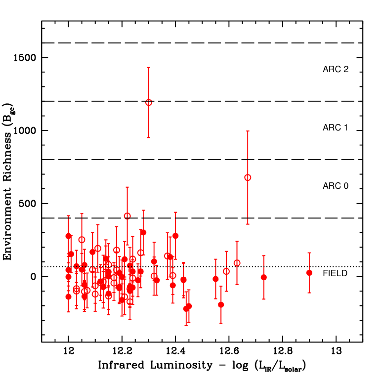
Figure 1:

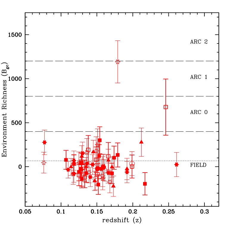
Figure 2:

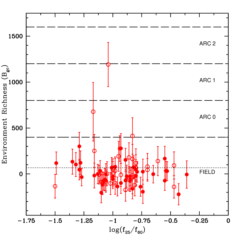
Figure 3:

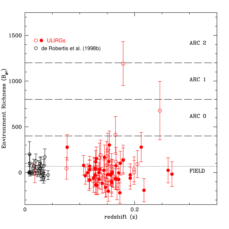
Figure 4:

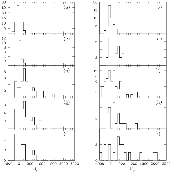
Figure 5:

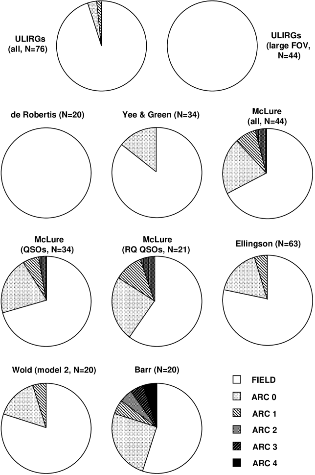
Figure 6:

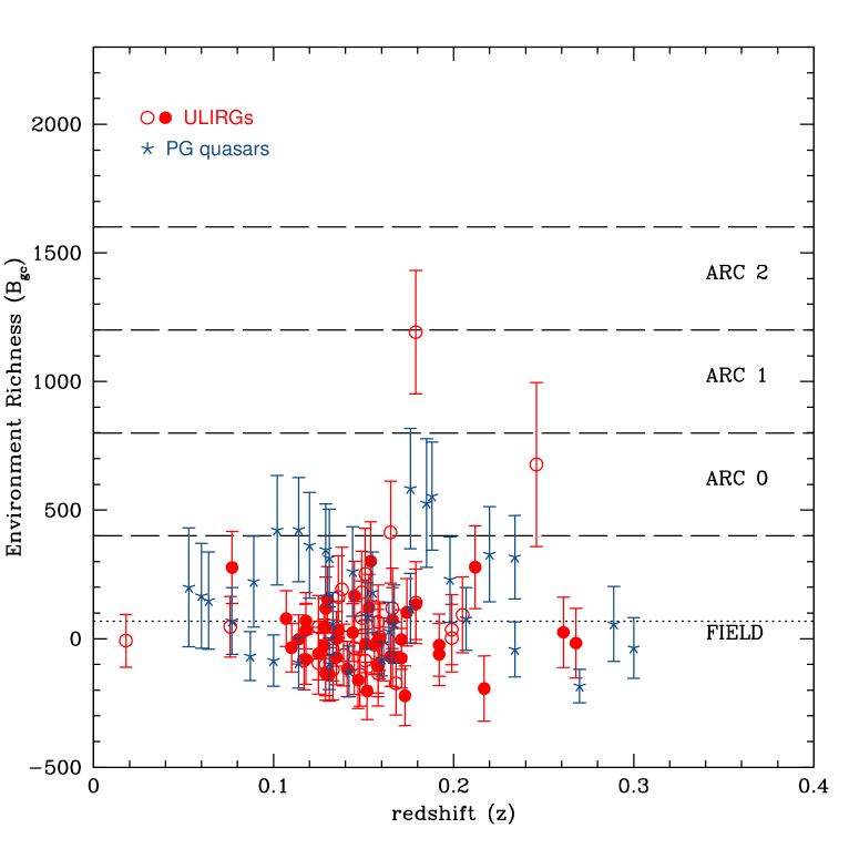
Figure 7:

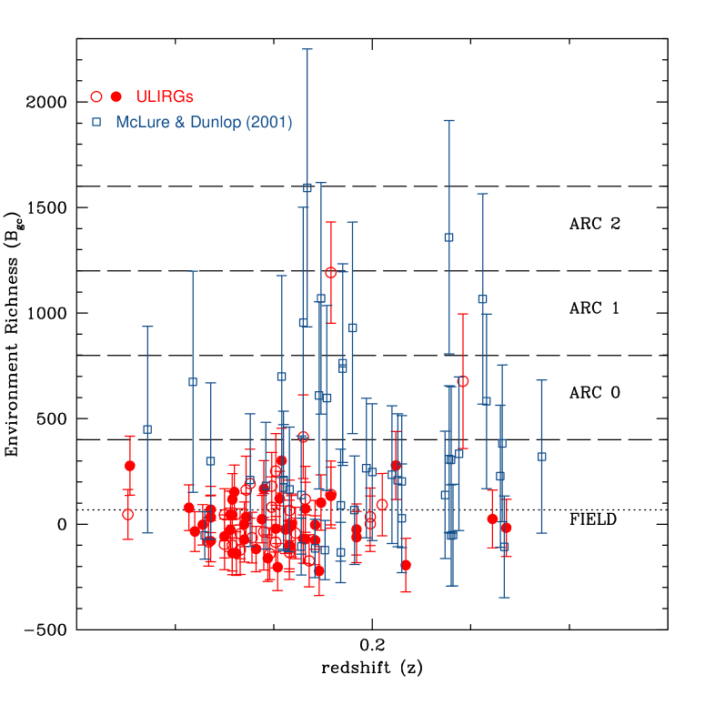
Figure 8:

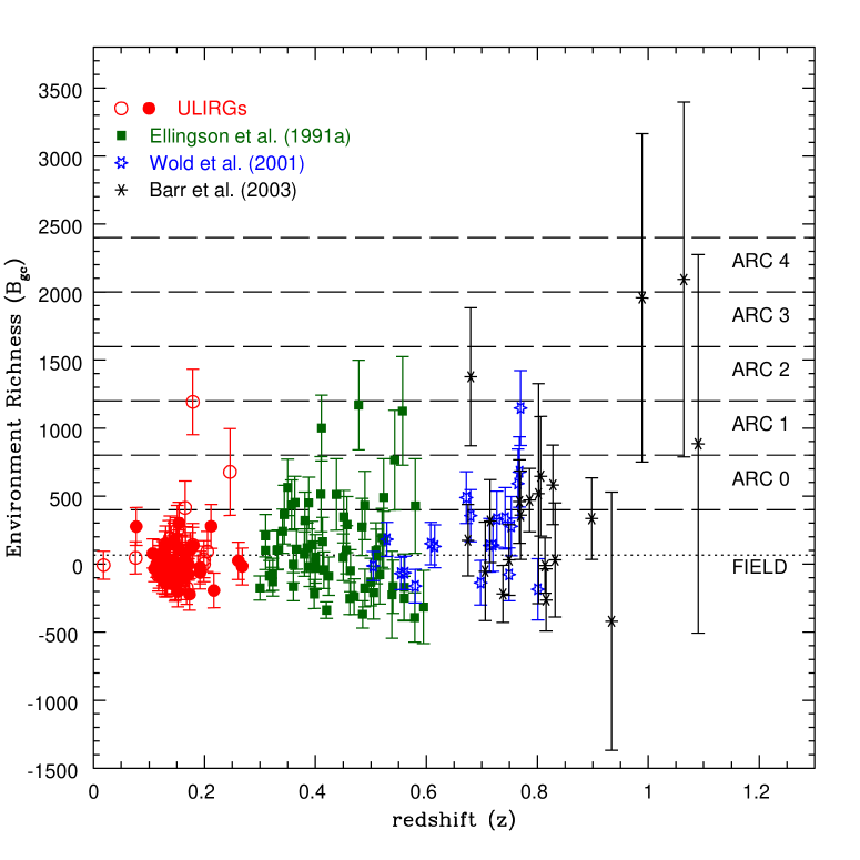
Figure 9:

References

- (1)
- (2) Andersen, V., & Owen, F. 1994, AJ, 108, 361
- (3) Barnes, J. E. 2004, MNRAS, 350, 798
- (4) Barr, J. M., Bremer, M. N., Baker, J. C., & Lehnert, M. D. 2003, MNRAS, 346, 229
- (5) Blain, A. W., Chapman, S. C., Smail, I., & Ivison, R. 2004, ApJ, 611, 725
- (6) Chapman, S. C., Blain, A. W., Smail, I., & Ivison, R. J. 2005, ApJ, 622, 772
- (7) Cowie, L. L., Barger, A. J., Fomalont, E. B., & Capak, P. 2004, ApJ, 603, L69
- (8) Croom, S. M., et al. 2005, MNRAS, 356, 415
- (9) Dasyra, K., et al. 2006a, ApJ, 638, 745
- (10) Dasyra, K., et al. 2006b, ApJ, in press (astro-ph/0607468)
- (11) Dasyra, K., et al. 2006c, ApJ, in press (astro-ph/0610719)
- (12) Davis, M., & Peebles, P. J. E. 1983, ApJ, 267, 465
- (13) de Robertis, M. M., Hayhoe, K., & Yee, H. K. C. 1998a, ApJS, 115, 163
- (14) de Robertis, M. M., Yee, H. K. C., & Hayhoe, K. 1998b, ApJ, 496, 93
- (15) Downes, D., & Solomon, P. M. 1998, ApJ, 507, 615
- (16) Dunlop, J. S., McLure, R. J., Kukula, M. J., Baum, S. A., O’Dea, C. P., & Hughes, D. H. 2003, MNRAS, 340, 1095
- (17) Ellingson, E., Yee, H. K. C., & Green, R. F. 1991, ApJ, 371, 49
- (18) Farrah, D., et al. 2004, MNRAS, 349, 518
- (19) Farrah, D., et al. 2006, ApJ, 641, L17
- (20) Genzel, R., Tacconi, L. J., Rigopoulou, D., Lutz, D., & Tecza, M. 2001, ApJ, 563, 527
- (21) Genzel, R., et al. 1998, ApJ, 498, 579
- (22) Gladders, M. D., & Yee, H. K. C. 2005, ApJS, 157, 1
- (23) Hill, G. J., & Lilly, S. J. 1991, ApJ, 367, 1
- (24) Hughes, D. H., et al. 1998, Nature, 394, 241
- (25) Kauffmann, G., et al. 2004, MNRAS, 353, 713
- (26) Kim, D.-C., & Sanders, D. B. 1998, ApJS, 119, 41
- (27) Kim, D.-C., Veilleux, S., & Sanders, D. B. 1998, ApJ, 508, 627
- (28) Kim, D.-C., Veilleux, S., & Sanders, D. B. 2002, ApJS, 143, 277
- (29) Kron, R. G. 1980, ApJS, 43, 305
- (30) Longair, M. S., & Seldner, M. 1979, MNRAS, 189, 433
- (31) Lonsdale, C. J., Farrah, D., & Smith, H. 2006, preprint (astro-ph/0603031)
- (32) Lutz, D., Veilleux, S., & Genzel, R. 1999, ApJ, 517, L13
- (33) Lutz, D., et al. 1998, ApJ, 505, L103
- (34) Martin, C. L. 2005, ApJ, 621, 227
- (35) McLure, R. J., & Dunlop, J. S. 2001, MNRAS, 321, 515
- (36) Mihos, J. C, & Hernquist, L. 1996, ApJ, 464, 641
- (37) Miller, C. J., Nichol, R. C., Gómez, P. L., Hopkins, A. M., & Bernardi, M. 2003, ApJ, 597, 142
- (38) Rigopoulou, D., et al. 1999, AJ, 118, 262
- (39) Rupke, D. S., Veilleux, S., & Sanders, D. B. 2002, ApJ, 570, 588
- (40) Rupke, D. S., Veilleux, S., & Sanders, D. B. 2005a, ApJS, 160, 115
- (41) Rupke, D. S., Veilleux, S., & Sanders, D. B. 2005b, ApJ, 632, 751
- (42) Sanders, D. B., & Mirabel, I. F. 1996, ARA&A, 34, 749
- (43) Sanders, D. B., et al. 1988, ApJ, 325, 74
- (44) Schmidt, M., & Green, R. F. 1983, ApJ, 269, 352
- (45) Scoville, N. Z., et al. 2000, AJ, 119, 991
- (46) Serber, W., Bahcall, N., Ménard, B., & Richards, G. 2006, ApJ, 643, 68
- (47) Smail, I., Ivison, R. J., & Blain, A. W. 1997, ApJ, 490, L5
- (48) Söchting, I. K., Clowes, R. B., & Campusano, L. E. 2004, MNRAS, 347, 1241
- (49) Soifer, B. T., et al. 2000, AJ, 119, 509
- (50) Soifer, B. T., et al. 2001, AJ, 122, 1213
- (51) Surace, J. A., & Sanders, D. B. 1999, ApJ, 512, 162
- (52) Surace, J. A., Sanders, D. B., & Evans, A. S. et al. 2001, AJ, 122, 2791
- (53) Tacconi, L. J., et al. 2002, ApJ, 580, 73
- (54) Tran, Q. D., et la. 2001, ApJ, 552, 527
- (55) Veilleux, S., Cecil, G., & Bland-Hawthorn, J. 2005, ARA&A, 43, 769
- (56) Veilleux, S., Kim, D.-C., & Sanders, D. B. 1999a, ApJ, 522, 113
- (57) Veilleux, S., Kim, D.-C., & Sanders, D. B. 2002, ApJS, 143, 315
- (58) Veilleux, S., Sanders, D. B., & Kim, D.-C. 1999b, ApJ, 522, 139
- (59) Veilleux, S., et al. 2006, ApJ, 643, 707
- (60) Waskett, T. J., Eales, S. A., Gear, W. K., McCracken, H. J., Lilly, S., & Brodwin, M. 2005, MNRAS, 363, 801
- (61) Wold, M., Lacy, M., Lilje, P. B., & Serjeant, S. 2000, MNRAS, 316, 267
- (62) Wold, M., Lacy, M., Lilje, P. B., & Serjeant, S. 2001, MNRAS, 323, 231
- (63) Yee, H. K. C. 1991, PASP, 103, 396
- (64) Yee, H. K. C., & Ellingson, E. 2003, ApJ, 585, 215
- (65) Yee, H. K. C., & Green, R. F. 1984, ApJ, 280, 79
- (66) Yee, H. K. C., & Green, R. F. 1987, ApJ, 319, 28
- (67) Yee, H. K. C., Green, R. F., & Stockman, H. S. 1986, ApJS, 63, 681
- (68) Yee, H. K. C., & López-Cruz, O. 1999, AJ, 117, 1985