Visualizing spacetimes via embedding diagrams

Abstract

It is hard to imagine curved spacetimes of General Relativity. A simple but powerful way how to achieve this is visualizing them via embedding diagrams of both ordinary geometry and optical reference geometry. They facilitate to gain an intuitive insight into the gravitational field rendered into a curved spacetime, and to assess the influence of parameters like electric charge and spin of a black hole, magnetic field or cosmological constant. Optical reference geometry and related inertial forces and their relationship to embedding diagrams are particularly useful for investigation of test particles motion. Embedding diagrams of static and spherically symmetric, or stationary and axially symmetric black-hole and naked-singularity spacetimes thus present a useful concept for intuitive understanding of these spacetimes’ nature. We concentrate on general way of embedding into 3-dimensional Euclidean space, and give a set of illustrative examples.

1 Introduction

The analysis of embedding diagrams (Stuchlík and Hledík, 1999a; Stuchlík et al., 2001; Kristiansson et al., 1998; Stuchlík and Hledík, 2002a, 1999b; Bardeen, 1973; Stuchlík, 2001; Slaný, 2001) rank among the most fundamental techniques that enable understanding phenomena present in extremely strong gravitational fields of black holes and other compact objects. The influence of charge, spin, magnetic field or cosmological constant on the structure of spacetimes can suitably be demonstrated by embedding diagrams of 2-dimensional sections of the ordinary geometry ($t=\mathrm{const}$ hypersurfaces) into 3-dimensional Euclidean geometry and their relation to the well known ‘Schwarzschild throat’ (Misner et al., 1973).

Properties of the motion of both massive and massless test particles can be properly understood in the framework of optical reference geometry allowing introduction of the concept of gravitational and inertial forces in the framework of general relativity in a natural way (Abramowicz et al., 1988, 1995; Abramowicz, 1990, 1992; Abramowicz and Bičák, 1991; Abramowicz and Miller, 1990; Miller, 1993; Abramowicz and Prasanna, 1990; Abramowicz et al., 1993a), providing a description of relativistic dynamics in accord with Newtonian intuition.

The optical geometry results from an appropriate conformal ($3+1$) splitting, reflecting certain hidden properties of the spacetimes under consideration through their geodesic structure. Let us recall the basic properties of the optical geometry. The geodesics of the optical geometry related to static spacetimes coincide with trajectories of light, thus being ‘optically straight’ (Abramowicz and Prasanna, 1990; Abramowicz et al., 1993b). Moreover, the geodesics are ‘dynamically straight,’ because test particles moving along them are held by a velocity-independent force (Abramowicz, 1990); they are also ‘inertially straight,’ because gyroscopes carried along them do not precess along the direction of motion (Abramowicz, 1992).

Some fundamental properties of the optical geometry can be appropriately demonstrated namely by embedding diagrams of its representative sections (Abramowicz et al., 1988; Kristiansson et al., 1998; Stuchlík and Hledík, 1999b). Because we are familiar with the Euclidean space, 2-dimensional sections of the optical space are usually embedded into the 3-dimensional Euclidean space. In spherically symmetric static spacetimes, the central planes are the most convenient for embedding – with no loss of generality one can consider the equatorial plane, choosing the coordinate system such that $\theta=\pi/2$. In Kerr–Newman backgrounds, the most representative section is the equatorial plane, which is the symmetry plane. This plane is also of great astrophysical importance, particularly in connection with the theory of accretion disks (Bardeen, 1973).

In spherically symmetric spacetimes (Schwarzschild (Abramowicz and Prasanna, 1990), Schwarzschild–de Sitter (Stuchlík and Hledík, 1999a), Reissner–Nordström (Kristiansson et al., 1998), and Reissner–Nordström–de Sitter (Stuchlík and Hledík, 2002a)), an interesting coincidence appears: the turning points of the central-plane embedding diagrams of the optical space and the photon circular orbits are located exactly at the radii where the centrifugal force, related to the optical space, vanishes and reverses sign. The same conclusion holds for the Ernst spacetime (Stuchlík and Hledík, 1999b).

However, in the rotating black-hole backgrounds, the centrifugal force does not vanish at the radii of photon circular orbits (Iyer and Prasanna, 1993; Stuchlík et al., 2000). Of course, the same statement is true if these rotating backgrounds carry a non-zero electric charge.

Throughout the paper, geometrical units ($c=G=1$) are used.

2 Optical geometry and inertial forces

The notions of the optical reference geometry and the related inertial forces are convenient for spacetimes with symmetries, particularly for stationary (static) and axisymmetric (spherically symmetric) ones. However, they can be introduced for a general spacetime lacking any symmetry (Abramowicz et al., 1993a).

Assuming a hypersurface globally orthogonal to a timelike unit vector field $n$ and a scalar field $\Phi$ satisfying the conditions $n_{[\kappa}\nabla\!_{\lambda}n_{\mu]}=0$, $n^{\kappa}n_{\kappa}=-1$, $\dot{n}_{\lambda}\equiv n^{\kappa}\nabla\!_{\kappa}n_{\lambda}=\nabla\!_{\lambda}\Phi$, the 4-velocity $u$ of a test particle of rest mass $m$ can be uniquely decomposed as

$$u^{\kappa}=\gamma(n^{\kappa}+v\tau^{\kappa})\,.$$ (1)

Here, $\tau$ is a unit vector orthogonal to $n$, $v$ is the speed, and $\gamma=(1-v^{2})^{-1/2}$.

Introducing, based on the approach of Abramowicz et al. (1993a), a projected 3-space orthogonal to $n$ with the positive definite metric $h_{\kappa\lambda}$ giving the so-called ordinary projected geometry, and the optical geometry $\tilde{h}_{\kappa\lambda}$ by conformal rescaling

$$\tilde{h}_{\kappa\lambda}=\mathrm{e}^{-2\Phi}h_{\kappa\lambda}\,,\qquad h_{\kappa\lambda}=g_{\kappa\lambda}+n_{\kappa}n_{\lambda}\,,$$ (2)

the projection of the 4-acceleration $a^{\bot}_{\kappa}=h^{\lambda}_{\kappa}\,u^{\mu}\nabla\!_{\mu}u_{\lambda}$ can be uniquely decomposed into terms proportional to the zeroth, first, and second powers of $v$, respectively, and the velocity change $\dot{v}=(\mathrm{e}^{\Phi}\gamma v)_{,\mu}\,u^{\mu}$. Thus, we arrive at a covariant definition of inertial forces analogous to the Newtonian physics (Abramowicz et al., 1993a; Aguirregabiria et al., 1996)

$$ma^{\bot}_{\kappa}=G_{\kappa}(v^{0})+C_{\kappa}(v^{1})+Z_{\kappa}(v^{2})+E_{\kappa}(\dot{v})\,,$$ (3)

where the terms

$$G_{\kappa}=-m\nabla\!_{\kappa}\Phi=-m\Phi\!_{,\kappa}\,,\quad C_{\kappa}=-m\gamma^{2}vn^{\lambda}(\nabla\!_{\lambda}\tau_{\kappa}-\nabla\!_{\kappa}\tau_{\lambda})\,,\quad Z_{\kappa}=-m(\gamma v)^{2}\tilde{\tau}^{\lambda}\tilde{\nabla}\!_{\lambda}\tilde{\tau}_{\kappa}\,,\quad E_{\kappa}=-m\dot{v}\tilde{\tau}_{\kappa}\,,$$ (4)

correspond to the gravitational, Coriolis–Lense–Thirring, centrifugal and Euler force, respectively. Here, $\tilde{\mbox{\boldmath$\tau$}}$ is the unit vector along $\tau$ in the optical geometry and $\tilde{\mbox{\boldmath$\nabla$}}$ is the covariant derivative with respect to the optical geometry.

In the simple case of static spacetimes with a field of timelike Killing vectors $\mbox{\boldmath$n$}\equiv\mbox{\boldmath$\xi$}_{(t)}=\partial/\partial t$, we are dealing with space components that we will denote by Latin indices in the following. The metric coefficients of the optical reference geometry are given by the formula

$$\tilde{h}_{ik}=\mathrm{e}^{-2\Phi}h_{ik}\,,\qquad\mathrm{e}^{2\Phi}=-g_{\mu\nu}\xi^{\mu}_{(t)}\xi^{\nu}_{(t)}=-g_{tt}\,.$$ (5)

In the optical geometry, we can define a 3-momentum of a test particle and a 3-force acting on the particle (Abramowicz et al., 1993a; Stuchlík, 1990)

$$\tilde{p}^{i}=\mathrm{e}^{2\Phi}p^{i}\,,\qquad\tilde{f}_{i}=\mathrm{e}^{2\Phi}f_{i}\,,$$ (6)

where $p^{i}$, $f_{i}$ are space components of the 4-momentum $p$ and the 4-force $f$. Instead of the full spacetime form, the equation of motion takes the following form in the optical geometry,

$$m\tilde{f}_{i}=\tilde{p}^{k}\tilde{\nabla}\!_{k}\tilde{p}_{i}+{\textstyle\frac{1}{2}}m^{2}\tilde{\nabla}\!_{i}\Phi\,,$$ (7)

where $\tilde{\nabla}\!_{k}$ represents the covariant derivative components with respect to the optical geometry. We can see directly that photon trajectories ($m=0$) are geodesics of the optical geometry. The first term on the right-hand side of (7) corresponds to the centrifugal force, the second one corresponds to the gravitational force.

In the case of Kerr–Newman spacetimes, detailed analysis (see, e.g., (Stuchlík et al., 2000)) leads to decomposition into gravitational, Coriolis–Lense–Thirring and centrifugal forces (4)

$$G_{\kappa} = -m\Phi\!_{,\kappa}=-m\frac{1}{2}\partial_{\kappa}\left[\ln\left(\frac{g^{2}_{t\phi}-g_{tt}g_{\phi\phi}}{g_{\phi\phi}}\right)\right]\,,$$ (8)

$$C_{\kappa} = mA^{2}(\Omega-\Omega_{\mathrm{LNRF}})\sqrt{g_{\phi\phi}}\left[\partial_{\kappa}\left(g_{t\phi}g_{\phi\phi}^{-1/2}\right)+\Omega_{\mathrm{LNRF}}\,\partial_{\kappa}\sqrt{g_{\phi\phi}}\right]\,,$$ (9)

$$Z_{\kappa} = -\frac{1}{2}mA^{2}(\Omega-\Omega_{\mathrm{LNRF}})^{2}g_{\phi\phi}\,\partial_{\kappa}\left[\ln\left(\frac{g^{2}_{\phi\phi}}{g^{2}_{t\phi}-g_{tt}g_{\phi\phi}}\right)\right]\,,$$ (10)

respectively; we also denote $\mbox{\boldmath$\iota$}=\mathrm{e}^{-\Phi}\mbox{\boldmath$n$}$. The Euler force will appear for $\Omega\neq\mathrm{const}$ only, being determined by $\dot{\Omega}=u^{\lambda}\nabla\!_{\lambda}\Omega$ (see (Abramowicz et al., 1995)). Here we shall concentrate on the inertial forces acting on the motion in the equatorial plane ($\theta=\pi/2$) and their relation to the embedding diagram of the equatorial plane of the optical geometry.

Clearly, by definition, the gravitational force is independent of the orbiting particle velocity. On the other hand, both the Coriolis–Lense–Thirring and the centrifugal force vanish (at any $r$) if $\Omega=\Omega_{\mathrm{LNRF}}$, i.e., if the orbiting particle is stationary at the LNRF located at the radius of the circular orbit; this fact clearly illustrates that the LNRF are properly chosen for the definition of the optical geometry and inertial forces in accord with Newtonian intuition. Moreover, both forces vanish at some radii independently of $\Omega$. In the case of the centrifugal force, namely this property will be imprinted into the structure of the embedding diagrams.

3 Embedding diagrams

The properties of the (optical reference) geometry can conveniently be represented by embedding of the equatorial (symmetry) plane into the 3-dimensional Euclidean space with line element expressed in the cylindrical coordinates ($\rho,z,\alpha$) in the standard form. The embedding diagram is characterized by the embedding formula $z=z(\rho)$ determining a surface in the Euclidean space with the line element

$$\mathrm{d}\ell^{2}_{\mathrm{(E)}}=\left[1+\left(\frac{\mathrm{d}z}{\mathrm{d}\rho}\right)^{2}\right]\mathrm{d}\rho^{2}+\rho^{2}\,\mathrm{d}\alpha^{2}$$ (11)

isometric to the 2-dimensional equatorial plane of the ordinary or the optical space line element (Stuchlík and Hledík, 1999c)

$$\mathrm{d}\ell^{2}=h_{rr}\,\mathrm{d}r^{2}+h_{\phi\phi}\,\mathrm{d}\phi^{2}.$$ (12)

The azimuthal coordinates can be identified ($\alpha\equiv\phi$) which immediately leads to $\rho^{2}=h_{\phi\phi}$, and the embedding formula is governed by the relation

$$\left(\frac{\mathrm{d}z}{\mathrm{d}\rho}\right)^{2}=h_{rr}\left(\frac{\mathrm{d}r}{\mathrm{d}\rho}\right)^{2}-1.$$ (13)

It is convenient to transfer the embedding formula into a parametric form $z(\rho)=z(r(\rho))$ with $r$ being the parameter. Then

$$\frac{\mathrm{d}z}{\mathrm{d}r}=\pm\sqrt{h_{rr}-\left(\frac{\mathrm{d}\rho}{\mathrm{d}r}\right)^{2}}.$$ (14)

The sign in this formula is irrelevant, leading to isometric surfaces. Because $\mathrm{d}z/\mathrm{d}\rho=(\mathrm{d}z/\mathrm{d}r)(\mathrm{d}r/\mathrm{d}\rho)$, the turning points of the embedding diagram, giving its throats and bellies, are determined by the condition $\mathrm{d}\rho/\mathrm{d}r=0$. The embedding diagram can be constructed if the reality condition $h_{rr}-(\mathrm{d}\rho/\mathrm{d}r)^{2}\geq 0$ holds.

4 Examples of embedding diagrams

In this section we present graphic representations of embedding diagrams for various spacetimes with their brief description. For full treatment, see the reference provided at the beginning of each subsection.

4.1 Schwarzschild spacetime with nonzero cosmological constant

The influence of cosmological constant on the structure of Schwarzschild–de Sitter spacetime is treated in full technical details by Stuchlík and Hledík (1999a). Putting $y\equiv\Lambda M^{2}/3$, $t\to t/M$, $r\to r/M$, where $M$ is the mass parameter and $\Lambda$ denotes the cosmological constant, the line element in standard Schwarzschild coordinates reads

$$\mathrm{d}s^{2}=-\left(1-\frac{2}{r}-yr^{2}\right)\mathrm{d}t^{2}+\left(1-\frac{2}{r}-yr^{2}\right)^{-1}\mathrm{d}r^{2}+r^{2}(\mathrm{d}\theta^{2}+\sin^{2}\theta\,\mathrm{d}\phi^{2})\,.$$ (15)

Embedding diagrams of the ordinary geometry are given by the formula $z=z(r)$, which can be obtained by integrating the relation

$$\frac{\mathrm{d}z}{\mathrm{d}r}=\left(\frac{2+yr^{3}}{r-2-yr^{3}}\right)^{1/2}\,.$$ (16)

In the case of Schwarzschild–de Sitter spacetimes, the embedding can be constructed for complete static regions between the black-hole ($r_{\mathrm{h}}$) and cosmological ($r_{\mathrm{c}}$) horizons. Recall that the static region exists for $y\leq 1/27$ only. In the case of Schwarzschild–anti-de Sitter spacetimes, the static region extends from the black-hole horizon to infinity. However, we can see directly from Eq. (16) that the embedding diagrams of the ordinary space can be constructed in a limited part of the static region, located between the black-hole horizon $r_{\mathrm{h}}$ and $r_{\rm e(ord)}=(-2/y)^{1/3}$.

Embedding diagrams of optical reference geometry are given by parametric formulas $z=z(r),\rho=\rho(r)$:

$$\frac{\mathrm{d}z}{\mathrm{d}r}=\frac{r}{r-2-yr^{3}}\left[\frac{4r-9-yr^{4}}{r(r-2-yr^{3})}\right]^{1/2}\,,\quad\rho=r\left(1-\frac{2}{r}-yr^{2}\right)^{-1/2}\,.$$ (17)

The embedding formula $z=z(\rho)$ can then be constructed by a numerical procedure. Further, it can be shown (Stuchlík and Hledík, 1999a) that ‘turning radii’ of the embedding diagrams are given by the condition $\mathrm{d}\rho/\mathrm{d}r=0$. Since

$$\frac{\mathrm{d}\rho}{\mathrm{d}r}=\left(1-\frac{3}{r}\right)\left(1-\frac{2}{r}-yr^{2}\right)^{-3/2},$$ (18)

we can see that the turning radius determining a throat of the embedding diagram of the optical geometry is located just at $r=3$, corresponding to the radius of the photon circular orbit; it is exactly the same result as that obtained in the pure Schwarzschild case. The radius of the photon circular orbit is important from the dynamical point of view, because the centrifugal force related to the optical geometry reverses its sign there (Abramowicz and Prasanna, 1990; Stuchlík, 1990). Above the photon circular orbit, the dynamics is qualitatively Newtonian with the centrifugal force directed towards increasing $r$. However, at $r=3$, the centrifugal force vanish, and at $r<3M$ it is directed towards decreasing $r$. The photon circular orbit, the throat of the embedding diagram of the optical geometry ($\mathrm{d}\rho/\mathrm{d}r=0$), and vanishing centrifugal force, all appear at the radius $r=3$.

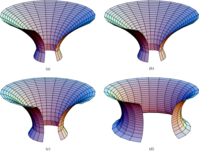
Figure 1: Left panel: Qualitative features of the embedding diagrams of the ordinary geometry of the Schwarzschild–de Sitter and Schwarzschild–anti-de Sitter spacetimes in a log-log diagram. One can immediately see how the diagrams with $y\neq 0$ ‘peel off’ the pure Schwarzschild diagram ($y=0$, bold curve). All sections with $y\neq 0$ are complete (i.e., the maximum that can be embedded into Euclidean space is shown), except uninteresting lower parts of the throats. The diagrams clearly indicate modifications of the spacetime structure caused by the presence of a cosmological constant. Middle panel: Same as left panel but for optical geometry. Right panel: Example of embedding diagrams of the optical reference geometry of the Schwarzschild–de Sitter spacetimes. The pure Schwarzschild case is taken for comparison in (a). The diagrams are given for (b) $y=10^{-6}$, (c) $y=0.002$, and (d) $y=0.03$. They are similar to the pure Schwarzschild case, because the region near the cosmological horizon being of highly different character is ‘cut off’ by the limit of embeddability. Taken from (Stuchlík and Hledík, 1999a).

In the case of Schwarzschild–de Sitter spacetimes containing the static region, the embeddability of the optical geometry is restricted both from below, and from above. Using a numerical procedure, the embedding diagrams are constructed for the same values of $y$ as in the case of the ordinary geometry.

In the case of Schwarzschild–anti-de Sitter spacetimes, the embeddability of the optical geometry is restricted from below again; with $y\to-\infty$ the limit shifts to $r\to 0$, along with the radius of the black-hole horizon. The embedding diagrams are constructed by the numerical procedure for the same values of $y$ as for the ordinary space. These diagrams have a special property, not present for the embedding diagrams in the other cases. Namely, they cover whole the asymptotic part of the Schwarzschild–anti-de Sitter spacetime, but in a restricted part of the Euclidean space. This is clear from the asymptotic behavior of $\rho(r)$. For $r\to+\infty$, there is $\rho\sim(-y)^{-1/2}$. Clearly, with decreasing attractive cosmological constant the embedding diagram is deformed with increasing intensity. The circles of $r=\mathrm{const}$ are concentrated with an increasing density around $\rho=(-y)^{-1/2}$ as $r\to\infty$.

Basic features of the embedding diagrams of the Schwarzschild–de Sitter spacetimes are illustrated in Figure 1.

4.2 Interior uniform-density Schwarzschild spacetime with nonzero cosmological constant

The influence of the cosmological constant on the structure of interior uniform-density Schwarzschild spacetime is treated in full technical details by Stuchlík et al. (2001).

The line element in standard Schwarzschild coordinates reads

$$\mathrm{d}s^{2}=-\mathrm{e}^{2\Phi(r)}\,\mathrm{d}t^{2}+\mathrm{e}^{2\Psi(r)}\,\mathrm{d}r^{2}+r^{2}(\mathrm{d}\theta^{2}+\sin^{2}\theta\,\mathrm{d}\varphi^{2})\,,$$ (19)

where

$$\mathrm{e}^{\Psi(r)}=\left(1-\frac{r^{2}}{a^{2}}\right)^{-1/2}\,,\;\mathrm{e}^{\Phi(r)}=A\mathrm{e}^{-\Psi(R)}-B\mathrm{e}^{-\Psi(r)}\,,\;\frac{1}{a^{2}}=\frac{2M}{R^{3}}+\frac{\Lambda}{3}\,,\;A=\frac{9M}{6M+\Lambda R^{3}}\,,\;B=\frac{3M-\Lambda R^{3}}{6M+\Lambda R^{3}}\,.$$ (20)

Here $M$ denotes total mass, $\rho$ (uniform) mass density and $R$ external radius of the configuration; $\Lambda$ is the cosmological constant. Examples of embedding diagrams (for repulsive cosmological constant) are shown in Figure 2.

Ordinary geometry

Optical geometry

Figure 2: Axial sections of the Schwarzschild–de Sitter ($\Lambda>0$) case. The dashed curve represents pure Schwarzschild spacetime, the dots mark the position of the edge of the internal spacetime (i.e., $r=R=xM$). The embedding diagrams of the optical reference geometry show the existence of internal circular null geodesics which play a key role for the possibility of neutrino trapping.

4.3 Reissner–Nordström spacetime with nonzero cosmological constant

This section is based on (Stuchlík and Hledík, 2002b), where full-detail treatment can be found. Putting $y\equiv{\textstyle\frac{1}{3}}\Lambda M^{2}$, $e\equiv Q/M$, $t\to t/M$, $r\to r/M$, where $M$ is the mass parameter, $Q$ is the electric charge and $\Lambda$ is the cosmological constant, the line element in standard Schwarzschild coordinates reads

$$\mathrm{d}s^{2}=-\left(1-\frac{2}{r}+\frac{e^{2}}{r^{2}}-y{r^{2}}\right)\mathrm{d}t^{2}+\left(1-\frac{2}{r}+\frac{e^{2}}{r^{2}}-y{r^{2}}\right)^{-1}\mathrm{d}r^{2}+r^{2}\left(\mathrm{d}\theta^{2}+\sin^{2}\theta\,\mathrm{d}\phi^{2}\right)\,.$$ (21)

An example of classification based on properties of embedding diagrams of optical reference geometry is in Figure 3.

Figure 3: An example classification of Reissner–Nordström spacetimes according to properties of embedding diagrams of optical reference geometry. Taken from (Stuchlík and Hledík, 2002b).

4.4 Ernst spacetime

The static Ernst spacetime (Ernst, 1976; Stuchlík and Hledík, 1999b) is the only exact solution of Einstein’s equations known to represent the spacetime of a spherically symmetric massive body or black hole of mass $M$ immersed in an otherwise homogeneous magnetic field. If the magnetic field disappears, the geometry simplifies to the Schwarzschild geometry. Therefore, sometimes the Ernst spacetime is called magnetized Schwarzschild spacetime. Usually it is believed that for extended structures like galaxies both the effects of general relativity and the role of a magnetic field can be ignored. However, in the case of active galactic nuclei with a huge central black hole and an important magnetic field, the Ernst spacetime can represent some relevant properties of the galactic structures. Therefore, it could even be astrophysically important to discuss and illustrate basic properties of the Ernst spacetime.

The Ernst spacetime has the important property that it is not asymptotically flat. Far from the black hole, the spacetime is closely related to Melvin’s magnetic universe, representing a cylindrically symmetric spacetime filled with an uniform magnetic field only. The Ernst spacetime is axially symmetric, and its structure corresponds to the structure of the Schwarzschild spacetime only along its axis of symmetry. Off the axis, the differences are very spectacular, and we shall demonstrate them for the equatorial plane, which is the symmetry plane of the spacetime.

The line element of the Ernst spacetime reads

$$\mathrm{d}s^{2}=\Lambda^{2}\left[-\left(1-\frac{2M}{r}\right)\mathrm{d}t^{2}+\left(1-\frac{2M}{r}\right)^{-1}\mathrm{d}r^{2}+r^{2}\,\mathrm{d}\theta^{2}\right]+\frac{r^{2}\sin^{2}\theta}{\Lambda^{2}}\,\mathrm{d}\phi^{2}\,,$$ (22)

where $M\equiv M_{\mathrm{cgs}}G/c^{2}$ is the mass, $B\equiv B_{\mathrm{cgs}}G^{1/2}/c^{2}$ is the strength of the magnetic field, $\Lambda\equiv 1+B^{2}r^{2}\sin^{2}\theta$.

The dimensionless product $BM\ll 1$ in astrophysically realistic situations. Really, $BM\sim 2\times 10^{-53}B_{\mathrm{cgs}}M_{\mathrm{cgs}}$. For example, in case of a black hole with $M=10^{9}M_{\odot}$ (typical for AGN), the value $BM\sim 1$ corresponds to $B_{\mathrm{cgs}}\sim 10^{11}$ Gauss, which is unrealistic. Some illustrative embedding diagrams are collected in Figure 4.

$B=0.2>B_{\mathrm{c}}$

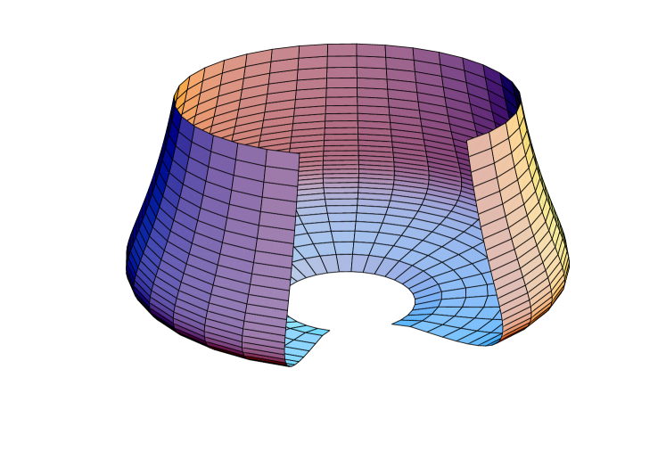
$B=0.08<B_{\mathrm{c}}$

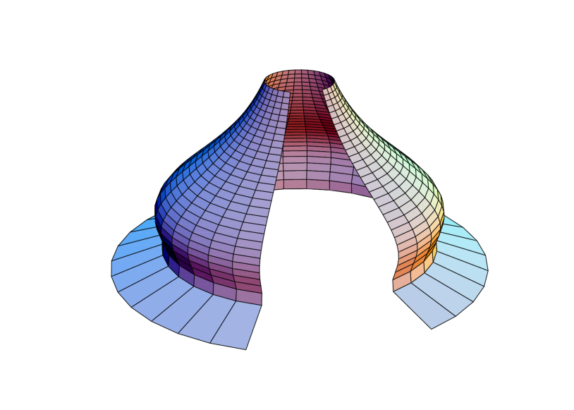
Figure 4: Left column: ordinary geometry, right column: optical geometry of Ernst spacetime. It can be proved (Stuchlík and Hledík, 1999b) that a critical magnetic field $B_{\mathrm{c}}\approx 0.0947$ exists. For $B>B_{\mathrm{c}}$, neither throats nor bellies and no circular photon orbits exist. For $B<B_{\mathrm{c}}$, the throat and the belly develop, corresponding to the inner unstable and outer stable photon circular orbit.

4.5 Kerr–Newman spacetimes

We focus on the results concerning the optical reference geometry (Stuchlík et al., 2000). It can be shown (Stuchlík et al., 2000) that the turning points of the embedding diagrams are really located at the radii where the centrifugal force vanishes and changes sign. Thus, we can conclude that it is exactly this property of optical geometry embeddings for the vacuum spherically symmetric spacetimes (see (Abramowicz et al., 1988; Kristiansson et al., 1998; Stuchlík and Hledík, 1999a)) survives in the Kerr–Newman spacetimes. However, photon circular orbits are displaced from the radii corresponding to the turning points of the embedding diagrams.

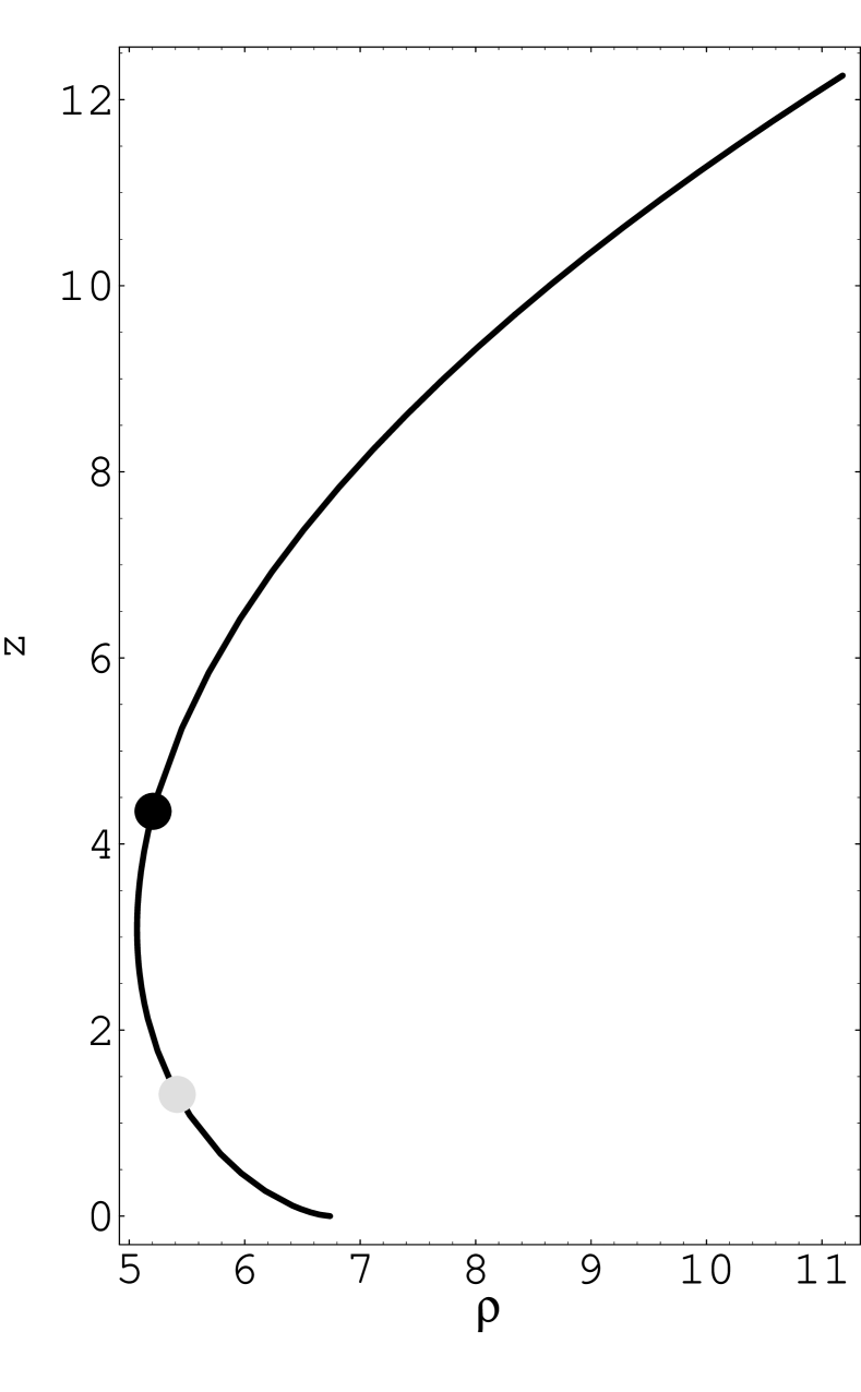
(a)

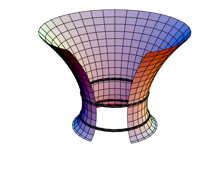
(b)

(c)

(d)

(e)

Figure 5: (a), (b): Embedding diagram of the Kerr–Newman black holes of the type BH₁, constructed for $a^{2}=0.16$, $e^{2}=0.16$. The rings in the 3D diagram represent photon circular orbits. Both corotating (gray spot in 2D diagram) and counterrotating (black spot in 2D diagram) orbits are displaced from the throat of the diagram where the centrifugal force vanishes. This is a general property of the rotating backgrounds. (c)–(e): Embedding diagrams of the black holes classes BH₂–BH₄. (c) Class BH₂ ($a^{2}=0.7$, $e^{2}=0.16$); (d) class BH₃ ($a^{2}=0.75$, $e^{2}=0.16$); (e) class BH₄ ($a^{2}=0.81$, $e^{2}=0.16$). Taken from (Stuchlík et al., 2000).

After a straightforward, but rather tedious, discussion, the full classification can be made according to the properties of the embedding diagrams (see (Stuchlík et al., 2000)).

Examples of typical black-hole embedding diagrams of classes labeled in Stuchlík et al. (2000) as BH₁–BH₄ are presented in Figure 5.

5 Concluding remarks

Embedding diagrams of the optical geometry give an important tool of visualization and clarification of the dynamical behavior of test particles moving along equatorial circular orbits: we imagine that the motion is constrained to the surface $z(\rho)$ (see (Kristiansson et al., 1998)). The shape of the surface $z(\rho)$ is directly related to the centrifugal acceleration. Within the upward sloping areas of the embedding diagram, the centrifugal acceleration points towards increasing values of $r$ and the dynamics of test particles has an essentially Newtonian character. However, within the downward sloping areas of the embedding diagrams, the centrifugal acceleration has a radically non-Newtonian character as it points towards decreasing values of $r$. Such a kind of behavior appears where the diagrams have a throat or a belly. At the turning points of the diagram, the centrifugal acceleration vanishes and changes its sign.

References

- Stuchlík and Hledík (1999a) Z. Stuchlík, and S. Hledík, Phys. Rev. D 60, 044006 (15 pages) (1999a).
- Stuchlík et al. (2001) Z. Stuchlík, S. Hledík, J. Šoltés, and E. Østgaard, Phys. Rev. D 64, 044004 (17 pages) (2001).
- Kristiansson et al. (1998) S. Kristiansson, S. Sonego, and M. A. Abramowicz, Gen. Relativity Gravitation 30, 275–288 (1998).
- Stuchlík and Hledík (2002a) Z. Stuchlík, and S. Hledík, Properties of the Reissner–Nordström spacetimes with a nonzero cosmological constant (2002a), unpublished, preprint TPA 003/Vol. 2, 2001.
- Stuchlík and Hledík (1999b) Z. Stuchlík, and S. Hledík, Classical Quantum Gravity 16, 1377–1387 (1999b).
- Bardeen (1973) J. M. Bardeen, “Timelike and Null Geodesics in the Kerr Metric,” in Black Holes, edited by C. D. Witt, and B. S. D. Witt, Gordon and Breach, New York–London–Paris, 1973, p. 215.
- Stuchlík (2001) Z. Stuchlík, “Accretion processes in black-hole spacetimes with a repulsive cosmological constant,” in Proceedings of RAGtime 2/3: Workshops on black holes and neutron stars, Opava, 11–13/8–10 October 2000/01, edited by S. Hledík, and Z. Stuchlík, Silesian University in Opava, Opava, 2001, pp. 129–167.
- Slaný (2001) P. Slaný, “Some aspects of Kerr–de Sitter spacetimes relevant to accretion processes,” in Proceedings of RAGtime 2/3: Workshops on black holes and neutron stars, Opava, 11–13/8–10 October 2000/01, edited by S. Hledík, and Z. Stuchlík, Silesian University in Opava, Opava, 2001, pp. 119–127.
- Misner et al. (1973) C. W. Misner, K. S. Thorne, and J. A. Wheeler, Gravitation, Freeman, San Francisco, 1973.
- Abramowicz et al. (1988) M. A. Abramowicz, B. Carter, and J. Lasota, Gen. Relativity Gravitation 20, 1173 (1988).
- Abramowicz et al. (1995) M. A. Abramowicz, P. Nurowski, and N. Wex, Classical Quantum Gravity 12, 1467 (1995).
- Abramowicz (1990) M. A. Abramowicz, Monthly Notices Roy. Astronom. Soc. 245, 733–746 (1990).
- Abramowicz (1992) M. A. Abramowicz, Monthly Notices Roy. Astronom. Soc. 256, 710–718 (1992).
- Abramowicz and Bičák (1991) M. A. Abramowicz, and J. Bičák, Gen. Relativity Gravitation 23, 941 (1991).
- Abramowicz and Miller (1990) M. A. Abramowicz, and J. C. Miller, Monthly Notices Roy. Astronom. Soc. 245, 729 (1990).
- Miller (1993) J. C. Miller, “Relativistic Gravitational Collapse,” in The Renaissance of General Relativity and Cosmology, edited by G. Ellis, A. Lanza, and J. Miller, Cambridge University Press, Cambridge, 1993, pp. 73–85, a Survey to Celebrate the 65th Birthday of Dennis Sciama.
- Abramowicz and Prasanna (1990) M. A. Abramowicz, and A. R. Prasanna, Monthly Notices Roy. Astronom. Soc. 245, 720–728 (1990).
- Abramowicz et al. (1993a) M. A. Abramowicz, P. Nurowski, and N. Wex, Classical Quantum Gravity 10, L183 (1993a).
- Abramowicz et al. (1993b) M. A. Abramowicz, J. Miller, and Z. Stuchlík, Phys. Rev. D 47, 1440–1447 (1993b).
- Iyer and Prasanna (1993) S. Iyer, and A. R. Prasanna, Classical Quantum Gravity 10, L13–L16 (1993).
- Stuchlík et al. (2000) Z. Stuchlík, S. Hledík, and J. Juráň, Classical Quantum Gravity 17, 2691–2718 (2000).
- Aguirregabiria et al. (1996) J. M. Aguirregabiria, A. Chamorro, K. R. Nayak, J. Suinaga, and C. V. Vishveshwara, Classical Quantum Gravity 13, 2179 (1996).
- Stuchlík (1990) Z. Stuchlík, Bull. Astronom. Inst. Czechoslovakia 41, 341 (1990).
- Stuchlík and Hledík (1999c) Z. Stuchlík, and S. Hledík, Acta Phys. Slovaca 49, 795–803 (1999c).
- Stuchlík and Hledík (2002b) Z. Stuchlík, and S. Hledík, Acta Phys. Slovaca 52, 363–407 (2002b).
- Ernst (1976) F. J. Ernst, J. Math. Phys. 17, 54 (1976).