Far-infrared to millimeter astrophysical dust emission

Abstract

Aims. We propose a new description of astronomical dust emission in the spectral region from the Far-Infrared to millimeter wavelengths.

Methods. Unlike previous classical models, this description explicitly incorporates the effect of the disordered internal structure of amorphous dust grains. The model is based on results from solid state physics, used to interpret laboratory data. The model takes into account the effect of absorption by Disordered Charge Distribution, as well as the effect of absorption by localized Two Level Systems.

Results. We review constraints on the various free parameters of the model from theory and laboratory experimental data. We show that, for realistic values of the free parameters, the shape of the emission spectrum will exhibit very broad structures which shape will change with the temperature of dust grains in a non trivial way. The spectral shape also depends upon the parameters describing the internal structure of the grains. This opens new perspectives as to identifying the nature of astronomical dust from the observed shape of the FIR/mm emission spectrum. A companion paper will provide an explicit comparison of the model with astronomical data.

1 Introduction

It is now well established that the Spectral Energy Distribution (SED) from the Inter-Stellar Medium (ISM) emission from our Galaxy and most external galaxies is dominated by thermal emission from dust grains which spans over almost 3 orders of magnitude in wavelengths, from the Near Infra-Red (NIR) to the millimeter wavelength range. Several dust models have been proposed to explain the observations. Recent dust models share many common characteristics (e.g. Mathis at al. Mathis77 (1977), Draine & Lee Draine84 (1984), Draine & Anderson Draine85 (1985), Weiland et al. Weiland86 (1986), Désert et al. Desert90 (1990), Li & Greenberg Li97 (1997), Dwek et al. Dwek97 (1997), Draine & Li Draine01 (2001)). Most of them require a wide range of the dust grain sizes spanning almost 3 orders of magnitude, from sub-nanometer dimensions to fractions of a micron. They also require a minimum of three components with different chemical composition in order to explain the ultraviolet and optical extinction, along with infrared emission.

The smallest component is needed to explain the ”aromatic” emission features at 3.3, 6.2, 7.7, 8.6 and $11.3\,{\rm\mu m}$. It is now routinely assigned to large aromatic molecules or Polycyclic Aromatic Hydrocarbons (PAH) (Leger & Puget Leger84 (1984), Allamandola et al. Allamandola85 (1985), Désert et al. Desert90 (1990)). PAH are transiently heated after absorbing single UV and far-UV photons, and cool down emitting NIR photons in vibrational transitions representative of their aromatic structure.

A second component, composed of Very Small Grains (VSG) is required to explain the continuum emission in the Mid Infra-Red (MIR). Emission in this range still requires significant temperature fluctuations of the grains, which necessitates, under conditions prevailing in the Inter-Stellar Medium (ISM), grains sizes in the nanometer range. VSGs could be composed of carbonaceous material whose absorption could also explain the $2200\AA$ UV bump in the extinction curve (see for instance Désert et al. Desert90 (1990)).

A third component, composed of Big Grains (BG), with sizes from 10-20 nm to about 100 nm, is necessary to account for the long wavelength emission (in particular as observed in the IRAS $100\,{\rm\mu m}$ band and above). The BG component dominates the total dust mass and the absorption in the visible and the NIR. Observations of the ”silicate” absorption feature near $10\,{\rm\mu m}$ indicate that their mass is dominated by amorphous silicates (see Kemper et al. Kemper04 (2004)). Such amorphous structure for these dust grains is expected from the interaction with cosmic rays which should alter the nature of the solid (Brucato et al. Brucato04 (2004), Jäger et al. Jager03 (2003)), but also from the formation processes of these BGs by aggregation of sub-sized particles.

Recent studies attempting to explain the submillimeter observations, revealed the need for either the existence of an additional most massive component of very cold dust (e.g. Reach et al. Reach95 (1995), Finkbeiner et al. Finkbeiner99 (1999), Galliano et al. Galliano03 (2003)) or for substantial modifications of dust properties in the submillimeter with respect to predictions of standard dust models (e.g. Ristorcelli et al. Ristorcelli98 (1998), Bernard et al. Bernard99 (1999), Stepnik et al. 2003a , Dupac et al. Dupac01G (2001), Dupac et al. Dupac02 (2002), Dupac et al. Dupac03 (2003)).

Similarly, laboratory spectroscopic measurements of interstellar grains analogs reveal that noticeable variations in their optical properties in the Far Infra-red (FIR) and Millimeter (mm) wavelength range can occur (Agladze et al. Agladze94 (1994), Agladze et al. Agladze96 (1996), Mennella et al. Mennella98 (1998), Boudet et al. Boudet05 (2005)). They pointed out the possible role of two phonons difference processes, disorder-induced one-phonon processes, resonant or relaxation processes in the presence of Two-Level Systems(TLS) in amorphous dust (see Sect. 4.3). The influence of such Two-Level Systems on interstellar grain absorption and emission properties was first proposed to the astronomers’s community by Agladze et al. Agladze94 (1994). More recently, a preliminary investigations by Boudet et al. Boudet02 (2002) showed that optical resonant and relaxation transitions in a distribution of TLS could qualitatively explain the anticorrelation between the temperature and the spectral index of dust as observed by the PRONAOS balloon experiment (e.g. Dupac et al. Dupac03 (2003)).

A precise modeling of the long wavelength dust emission is important in order to accurately subtract foreground emission in cosmological background anisotropy measurements, especially for future missions for space CMB measurements (Lamarre et al. Lamarre03 (2003)) and for surveys of foreground compact sources (see Gromov et al. Gromov02 (2002)). A number of comprehensive foreground analysis papers (Bouchet & Gispert Bouchet99 (1999), Tegmark et al. Tegmark00 (2000), Bennett et al. Bennett03 (2003), Barreiro et al. Barreiro04 (2006), Naselsky et al. Naselsky05 (2005) and other) did not pay attention to dust emissivity model accuracy. In addition, precise modeling of the FIR/mm dust emission is also important to derive reliable estimates of the dust mass, to trace the structure and density of pre-stellar cold cores in molecular clouds. Indeed the dust governs the cloud opacity, and influences the size of the cloud fragments. In addition, the efficiency of star formation should be related to the dust properties, which are expected to vary between the diffuse medium and the denser cold cores. It is thus of importance to know how some physical or chemical properties of dust can influence their FIR/mm emission.

For models of the submillimeter electromagnetic emission of dust, considering the intrinsic mechanical vibrations of the grain structure is natural since they fall in the right frequency range (typically in the frequency range $\nu\sim 10^{11}-10^{13}$ Hz, i.e. $\lambda\rm\sim 30\,{\rm\mu m}-3\,mm$). Observations in this spectral region potentially provides new tools for investigating the internal structure of dust grain material. The internal mechanics of grains is also important for chemistry in the ISM. The dust vibrations supply an energy sink for newly formed molecules which are usually formed in unstable excited states. Understanding the grain structure and intrinsic movements is necessary for considerations regarding grain collisions, destruction and agglomeration, including preplanetary bodies formation in circumstellar disks.

In Sect. 2, we first recall some basics regarding the FIR/mm dust emission and the semi-classical model of light interaction with matter. In Sect. 3, we gather evidences for spectral variations in astronomical and laboratory measurements. Then, we present in Sect. 4 a model, based on the intrinsic properties of amorphous materials, taking into account absorption by Disordered Charge Distribution as well as the effect of absorption by a distribution of TLS. In Sect. 5, we propose a new model of the submillimeter and millimeter grain absorption and discuss the range of plausible values for the free parameters, based on existing laboratory data. In Sect. 5.4, we discuss the implications of the model, in particular regarding the expected variations of the FIR/mm emission spectra with the dust temperature. Sect. 6 is devoted to conclusions. The determination of the model parameters applicable to astronomical data will addressed in a companion paper.

2 Basic knowledge on the FIR/mm dust emission

2.1 Interstellar dust emission and extinction

The intensity of thermal emission from interstellar dust at temperature $T_{\rm d}$ is

$$I_{\omega}(\omega,T)=\epsilon_{\rm e}(\omega)\cdot B_{\omega}(\omega,T_{\rm d})$$ (1)

where $I_{\omega}$ is energy flux density per unit area, angular frequency and solid angle (or specific intensity), $\epsilon_{\rm e}$ the dust emissivity and $B_{\omega}$ the Planck function at angular frequency $\omega$.

According to the Kirchhoff law, the emissivity $\epsilon_{\rm e}$ is equal to the absorptivity

$$\epsilon_{\rm e}(\omega)=1-e^{-\tau(\omega)}.$$ (2)

where the optical depth $\tau$ is related to the dust mass column density on the line of sight $M_{d}$ and the dust mass opacity $\kappa$ as

$$\tau(\omega)=\kappa(\omega)\cdot M_{d}$$ (3)

For spherical grains of radius $a$ and density $\rho$, the dust opacity (effective area per mass) is given by

$$\kappa(\omega)=\frac{3}{4\rho}\frac{Q(\omega)}{a},$$ (4)

where the absorption efficiency $Q(\omega)=\sigma(\omega)/(\pi a^{2})$ is the ratio of the absorption cross section $\sigma(\omega)$ to the geometrical cross section of the grain $\pi a^{2}$. The grain equilibrium temperature $T_{\rm d}$ is deduced from the balance between the emitted and absorbed radiation from the Inter-Stellar Radiation Field (ISRF)

$$\int^{\infty}_{0}B_{\omega}(\omega,T_{\rm d})Q(\omega)\mathrm{d}\omega=\int^{\infty}_{0}I^{ISRF}_{\omega}Q(\omega)\mathrm{d}\omega$$ (5)

The Mie theory, using the Maxwell equations of the electromagnetic theory, leads to an exact solution for the absorption and scattering processes by an homogeneous spherical particle of radius a whose material is characterized by its complex dielectric constant $\epsilon(\omega)=\epsilon^{\prime}(\omega)+i\epsilon^{\prime\prime}(\omega)$. In that case, the absorption coefficient $Q(\omega)$ writes as an infinite series of terms related to the complex dielectric constant. For particles small compared with the wavelength such as $|\sqrt{\epsilon(\omega)}|\cdot 2\pi a/\lambda\ll 1$ (where $\lambda=2\pi c/\omega$ is the wavelength and $c$ the speed of light in vacuum), the absorption coefficient can be approximated by

$$Q(\omega)=\frac{8\pi a}{\lambda}\cdot{\rm Im}\left[\frac{\epsilon(\omega)-1}{\epsilon(\omega)+2}\right]$$ (6)

In the FIR/mm wavelength range, for nonconducting materials of astronomical dust particles , the condition $\epsilon^{\prime\prime}\ll\epsilon^{\prime}$ is generally satisfied, and in this case the absorption coefficient reduces to

$$\frac{Q(\omega)}{a}=\frac{\omega}{c}\frac{12}{(\epsilon^{\prime}+2)^{2}}\epsilon^{\prime\prime},$$ (7)

As a consequence, following Eq. (7) the dust opacity rewrites

$$\kappa(\omega)=\frac{\omega}{c}\frac{9}{(\epsilon^{\prime}+2)^{2}}\frac{\epsilon^{\prime\prime}}{\rho}.$$ (8)

2.2 Assumption of a $\lambda$-independent emissivity spectral index

In the absence of specific knowledge about realistic dependencies for $\epsilon(\omega)$, a simple power law approximation for FIR/mm dust emission is often assumed

$$\kappa(\omega)=\kappa(\omega_{0})\left(\frac{\omega}{\omega_{0}}\right)^{\beta},$$ (9)

where $\beta$ is referred to as the emissivity spectral index.

The intensity of thermal emission from interstellar dust, assuming an optically thin medium, at a given wavelength $\lambda=2\pi/\omega$ located in the FIR/mm range is

$$I_{\omega}(\omega,T)=\epsilon_{\rm e}(\lambda_{0})\cdot\left(\frac{\omega}{\omega_{0}}\right)^{\beta}\cdot B_{\omega}(\omega,T_{\rm d})$$ (10)

where $\epsilon_{\rm e}(\lambda_{0})$ is the dust emissivity at a reference wavelength $\lambda_{0}=2\pi c/\omega_{0}$.

Simple semi-classical models of absorption such as the Lorentz model for damping oscillators and the Drude model for free charge carriers (Sect. 2.4) provide an asymptotic value $\beta=2$ when $\omega\rightarrow 0$. Such a value of the spectral index was in satisfactory agreement with the earliest observations of the FIR/mm SED of interstellar dust emission, but not necessarily with the most recent ones.

The emissivity spectral index $\beta$ is equal to the slope of a plot of the dust opacity versus wavelength in logarithmic scale. In the general case, the power-law assumption is not valid, and the spectral index has to be considered as a wavelength and temperature dependent parameter. Similarly, $\epsilon_{\rm e}(\lambda_{0})$ in Eq. (10) should be considered a function of $T$.

2.3 Relations between absorption properties of bulk material and dust

The absorption coefficient defined as the optical depth in the bulk material per unit length is

$$\alpha=2\mathrm{Im}(k),$$ (11)

where $k$ is the complex value of the wave number $k=\omega\sqrt{\epsilon}/c$ and $\epsilon$ is the complex dielectric constant Therefore for $\epsilon^{\prime\prime}\ll\epsilon^{\prime}$,

$$\alpha=\frac{\omega\epsilon^{\prime\prime}}{c\sqrt{\epsilon^{\prime}}}$$ (12)

In dust and porous material measurements, a mass absorption coefficient $\alpha/\rho$ is also often used.

In the following analysis (Sect. 2.4 and other) we will link the macroscopic value $\epsilon$ to the value of the local susceptibility $\chi_{o}=\chi_{o}^{\prime}+i\chi_{o}^{\prime\prime}$ defined on microscopic scale.

Because small astronomical particles cannot always be considered as a continuous medium, the electrodynamic equations of continuous media must be applied with care. So we detail in the following the equations used, and we discuss their range of application.

The Equations of motion describes the response of charges to a local electric field $\@vec{E_{0}}$, which permits to determine a dipole moment per unit volume as $\@vec{P}=\chi_{0}\@vec{E_{0}}$. It should be taken into account that the local electric field $\@vec{E_{0}}$ differs from an external field $\@vec{E}$ due to additional field produced by other parts of the dielectric. In the case of isotropic dielectric materials,

$$\@vec{E_{0}}=\@vec{E}+\frac{4\pi}{3}\@vec{P}.$$

The dielectric constant $\epsilon$ links the external field $\@vec{E}$ and the electric inductance $\@vec{D}=\@vec{E}+4\pi\@vec{P}$ through $\@vec{D}=\epsilon\@vec{E}$. In this case, $\epsilon$ can be derived from the susceptibility $\chi_{0}$, using the so called Clausius-Mossotti equation

$$\epsilon=1+\frac{4\pi\chi_{0}}{1-\frac{4}{3}\pi\chi_{0}}.$$ (13)

When $\epsilon^{\prime\prime}\ll\epsilon^{\prime}$, we have

$$\epsilon^{\prime\prime}\approx\frac{(\epsilon^{\prime}+2)^{2}}{9}\;4\pi\chi_{o}^{\prime\prime},$$ (14)

which leads to

$$\alpha(\omega) = \frac{4\pi\omega}{c\sqrt{\epsilon^{\prime}}}\frac{(\epsilon^{\prime}+2)^{2}}{9}\;\chi_{o}^{\prime\prime}(\omega),$$ (15)

$$\kappa(\omega) = \frac{\omega}{c}\frac{4\pi\chi_{o}^{\prime\prime}}{\rho}.$$ (16)

In Eq. (15), the term $(\epsilon^{\prime}+2)^{2}/9$ is the local field correction factor, the term $\sqrt{\epsilon^{\prime}}$ is the refraction index.

Thus, the relation between the absorption coefficient $\alpha$ deduced from transmission measurements in the laboratory and the absorption efficiency $Q$ or opacity $\kappa$, for small spherical grains of radius $a$ and density $\rho$ can be obtained from equations Eq. 7 and 12, and writes

$$\frac{Q(\omega)}{\alpha(\omega)}=\frac{12a\cdot\sqrt{\epsilon^{\prime}}}{(\epsilon^{\prime}+2)^{2}}$$ (17)

and as a consequence

$$\frac{\kappa(\omega)}{\alpha(\omega)}=\frac{9\cdot\sqrt{\epsilon^{\prime}}}{\rho\cdot(\epsilon^{\prime}+2)^{2}}$$ (18)

The condition $\epsilon^{\prime\prime}\ll\epsilon^{\prime}$ is valid for dust materials in the FIR/mm wavelength range, implying that the real part of the dielectric constant $\epsilon^{\prime}$ can be considered to first order as a constant, leading to $d\epsilon^{\prime}/d\omega=0$. This comes from the coupling between the real part $\epsilon^{\prime}$ and the imaginary part $\epsilon^{\prime\prime}$ through the Kramers-Kronig relations exposed in Sect. 3.2. This implies that, in that spectral range, the absorption coefficient $\alpha$, the absorption efficiency Q and the opacity $\kappa$ are simply proportional. Thus the slopes of $\alpha(\omega)$, Q$(\omega)$ and $\kappa(\omega)$ are the same. As for the emissivity, an absorptivity spectral index can then be defined by the slope of the spectral plot of the absorption $\alpha(\omega)$ in logarithmic scale. This absorptivity spectral index deduced from laboratory transmission measurements can be directly compared to the emissivity spectral index deduced from astrophysical measurements.

2.4 The semi-classical models

The well known semi-classical model of light interaction with charge carriers in matter (electrons and ions) considers the motion of charged particles driven by the time-dependent electric field of a monochromatic plane wave, magnetic forces being neglected compared with electrical forces.

The equations of motion of interacting charge carriers are:

$$m_{j}\ddot{u}_{j}^{\,\xi}+\sum_{j^{\prime}\xi^{\prime}}K_{jj^{\prime}}^{\xi\xi^{\prime}}u_{j^{\prime}}^{\,\xi^{\prime}}+\sum_{j^{\prime}\xi^{\prime}}b_{jj^{\prime}}^{\xi\xi^{\prime}}\dot{u}_{j^{\prime}}^{\,\xi^{\prime}}=q_{j}E^{\xi}(t),$$ (19)

where $m_{j}$, $q_{j}$ are masses and charges of particles, $K_{jj^{\prime}}^{\xi\xi^{\prime}}$ are constants of elastic interaction, $E^{\xi}$ is $\xi$-th component of electrical field vector $\@vec{E},\ u_{j}^{\xi}$ are components of the 3-dimensional vector of $j$-th ion displacement. Damping parameters $b_{j}$ describes dissipation of energy. Force constants $K$ are the coefficients of power expansion of the potential energy $U$.

$$U=\frac{1}{2}\sum_{j^{\prime}\xi^{\prime}}K_{jj^{\prime}}^{\xi\xi^{\prime}}u_{j}^{\xi}u_{j^{\prime}}^{\xi^{\prime}}+...$$ (20)

$U(\cdots u_{j}^{\xi}\cdots)$ depends only on relative deviations $(u_{j}^{\xi}-u_{j^{\prime}}^{\xi})$ with corresponding symmetry of $K_{jj^{\prime}}^{\xi\xi^{\prime}}$, particularly

$$K_{jj^{\prime}}^{\xi\xi^{\prime}}=K_{j^{\prime}j}^{\xi^{\prime}\xi},\ \sum_{j^{\prime}\xi^{\prime}}K_{jj^{\prime}}^{\xi\xi^{\prime}}=0.\$$ (21)

Linear Eq. (19) with $\@vec{E}=0$ have solutions in the form of a sum of damping oscillations

$$\@vec{u}=\sum a_{\kappa}\@vec{e}_{\kappa}\cdot\exp(-\gamma_{\kappa}t+i\omega_{\kappa}t),$$ (22)

where

$\@vec{u}=(\cdots u_{\kappa j}^{\ \xi}\cdots)$ is the multidimensional deviation vector, $a_{\kappa}$ are constants, $\@vec{e}_{\kappa}=(\cdots e_{\kappa j}^{\ \xi}\cdots)$ are eigenvectors, and $\gamma_{\kappa}-i\omega_{\kappa}$ are eigenvalues of matrix

$$\|-m_{j}\delta_{jj^{\prime}}\delta^{\xi\xi^{\prime}}+K_{jj^{\prime}}^{\xi\xi^{\prime}}+i\ b_{jj^{\prime}}^{\xi\xi^{\prime}}\|.$$ (23)

A solution of Eq. (19) with $\@vec{E}(t)=\hat{\@vec{E}}e^{-i\omega t}$ is $\@vec{u}=\hat{\@vec{u}}e^{-i\omega t},$

$$\hat{\@vec{u}}=\sum_{\kappa\ j}\frac{q_{j}\hat{\@vec{E}}\cdot\@vec{e}_{\kappa j}^{*}\ \omega_{\kappa}^{2}}{\omega_{\kappa}^{2}-\omega^{2}-i\gamma_{\kappa}\omega}.$$ (24)

Dielectric properties of a substance can be described by a susceptibility $\chi_{0}$, which is the dipole moment per unit volume generated by a unity local strenght $|\hat{\@vec{E}}|=1$ electrical field,

$$\chi_{o}=\sum_{\kappa}\frac{\rho_{\kappa}\omega_{\kappa}^{2}}{\omega_{\kappa}^{2}-\omega^{2}-i\gamma_{\kappa}\omega}.$$ (25)

For isotropic materials, constants

$$\rho_{\kappa}=\Big{|}\sum_{j\ j^{\prime}}q_{j^{\prime}}q_{j}\@vec{e}_{\kappa j^{\prime}}(\hat{\@vec{E}}\cdot\@vec{e}_{\kappa j}^{*})\Big{|}$$ (26)

does not depend upon the direction of $\hat{\@vec{E}}$.

In the extreme case where $\omega_{\kappa}\gg\gamma_{\kappa}$ the spectrum of the dielectric absorption can be described as a collection of non-overlapping resonant Lorentz profiles

$$\chi_{o}^{\prime\prime}=\frac{\rho_{\kappa}\omega_{\kappa}^{2}\gamma_{\kappa}\omega}{(\omega_{\kappa}^{2}-\omega^{2})^{2}+(\gamma_{\kappa}\omega)^{2}}.$$ (27)

It is the case of infrared absorption bands, especially in ionic crystals (”reststralen” bands). This corresponds to the third term of Eq. (19) being small.

In the opposite case ($\omega_{\kappa}\ll\gamma_{\kappa}$) this leads to a Debye relaxation spectrum when $\omega\ll\omega_{\kappa}$ :

$$\chi_{o}^{\prime\prime}=\frac{\rho_{\kappa}\ (\omega\tau_{\kappa})}{1+(\omega\tau_{\kappa})^{2}},$$ (28)

where $\tau_{\kappa}=\gamma_{\kappa}/\omega_{\kappa}^{2}$ is a relaxation constant. This is usually the case of polar dielectric liquids. It corresponds to the first term of Eq. (19) being negligible.

This spectrum corresponds to situations where the inertial effects (first term in Eq. 19) are comparatively small. If this condition is satisfied, the time constant in Eq. (28) can usually be determined by measuring or calculating the timescale of energy dissipation during return to equilibrium state, without solving Eq. (19).

A third extreme case, corresponding to the second term of Eq. (28) being negligible is usually refered to as the Drude approximation. It applies to free carriers and is considered in Sect. 2.6.

2.5 The Lorentz model for crystalline insulators

The Lorentz model applies for crystalline isolators with an ionic character, and describes the resonant interaction of an electromagnetic wave with the vibrations of ions which act like bound charges. Such an interaction is caused by the electric dipoles which arise when positive and negative ions move in opposite direction in their local electric field. This kind of dust absorption can be clearly identified in astrophysical observations as emission or absorption bands. Indeed, the optical depth $\tau$ is proportional to opacity $\kappa$ (Eq. 16):

$$\kappa(\omega)=\frac{4\pi}{c\rho}\sum_{\kappa}\frac{\rho_{\kappa}\omega_{\kappa}^{2}\gamma_{\kappa}\omega^{2}}{(\omega_{\kappa}^{2}-\omega^{2})^{2}+(\gamma_{\kappa}\omega)^{2}}$$ (29)

The maximum number of optically active vibrational modes in a crystal is $n_{opt}=3(s-1)$, where $s$ is the number of atoms in an elementary cell of the lattice. They are usually classified as branches in dispersion dependence of oscillation frequency $\omega(k)$ on wave number $k$. All these branches are restricted by relatively high $\omega(k)$ in the infrared region. Another 3 branches with $\omega(k)\rightarrow 0$ when $k\rightarrow$0 are acoustic modes. They are optically not active in crystal because a total charge of cell is zero. Another situation for amorphous matter is considered here in Sect. 4.2.

For substances of astrophysical interest, the characteristic frequencies of bands fall in region $\lambda\la 50\,{\rm\mu m}$. Therefore, in the FIR/mm wavelength range, the asymptotic $\omega\rightarrow 0$ of Eq. (29) can be used:

$$\kappa(\omega)=\omega^{2}\ \frac{4\pi}{c\rho}\sum_{\kappa}\frac{\rho_{\kappa}\gamma_{\kappa}}{\omega_{\kappa}^{2}}$$ (30)

Thus, the Lorentz model formally applied to dust in the FIR/mm wavelength range gives a spectral index $\beta=2$, a value often used in ”standard” dust models.

Many dust models have related the long wavelength absorption by interstellar silicates and ices ($\lambda>100\,{\rm\mu m}$) to the damping wing of the infrared-active fundamental vibrational bands, visible at shorter waves (see for example Andriesse et al. Andriesse74 (1974) and references therein).

Laboratory infrared data are satisfactorily described (see for example Rast Rast68 (1968)) by a sum of resonant Lorentz profiles (or reststrahlen bands) as described by Eq. (25) and Eq. (29), in which the various constants $\rho_{\kappa}$, $\omega_{\kappa}$, $\gamma_{\kappa}$ are determined from spectroscopic measurements. This model gives a satisfactory approximation for the infrared region, not only for ionic crystals, but also for covalent ones and for their amorphous counterparts with an appropriate choice of $\rho_{\kappa}$, $\omega_{\kappa}$, $\gamma_{\kappa}$.

The situation is more complicated for the low frequency region, where absorption is defined by damping constant $\gamma$, in contrast to IR bands, where absorption is weakly dependent on $\gamma$. The damping constants $b_{j}$ introduced in the semi-classical model (Eq. 19) and therefore $\gamma_{\kappa}$ in Eq. (29) have no simple microscopic explanation. The damping is linked to heating or distribution of energy to all modes of grain vibrations. So $\gamma$ characterizes intermode interactions which are frequency and temperature dependent in general. In contrast to single phonon absorption of resonant IR photons, a wing absorption is a two phonon difference process. Due to the conservation of energy, the energy of the absorbed low frequency photon is equal to the energy difference of the two phonons in the fundamental vibrational bands (Rubens and Hertz Rubens12 (1912), Ewald Ewald22 (1922)). In fact in crystals, any combination of acoustical and optical phonons which satisfies the energy and momentum conservation rules can take part to the absorption . This is the main source of infrared absorption in homoatomic crystals. In the FIR wavelength range the two-phonon difference processes are responsible for the absorption in ionic crystals. Because the efficiency of such processes are entirely determined by the difference between the phonon occupation numbers of the two involved phonons, the corresponding absorption decreases drastically at decreasing temperatures (Hadni Hadni70 (1970)).

However the optical behavior of amorphous materials is different. The disorder of the atomic arrangement leads to a breakdown of the selection rules for the wavenumber. The absorption spectra reflects thus the whole density of vibrational states. This induces in the longest wavelength range a broad absorption band due to single phonon processes which completely dominates over the multiphonon absorption (H. Henning and H. Mutschke Henning97 (1997)). As a consequence, such lattice absorption does not vanish at low temperature for the amorphous solids , in contrast to the crystalline ones.

2.6 The Drude model for conducting materials

For free charge carriers the previous semi-classical equation of motion (Eq. 19) can still be used, setting all restoring force coefficients $K$ to zero, equaling all the masses $m_{j}$ to the effective mass of the free carriers $m_{c}$ ( $m_{j}=m_{c}$), and using a constant value for the damping parameters $b_{j}/m_{j}$=const=$\gamma_{c}$. Therefore Eq. (25) for the susceptibility simplifies as $\chi_{o}=-\ \omega_{p}^{2}\ (\omega^{2}-i\gamma_{c}\omega)^{-1}$, where $\omega_{p}$ is the so-called plasma frequency $\omega_{p}^{2}=N_{c}q_{c}^{2}/m_{c}$, and $N_{c}$ is the number of free carriers per unit volume.

In metals, the number of free electrons per unit volume is independent of temperature, and is of the same order of magnitude than the number of atoms ($N_{c}\sim\ 10^{22}$ cm^-3). This leads to a frequency $\omega_{p}\sim 10^{15}$ s^-1 located in ultraviolet or in the visible, and to correspondingly high conductivity $\sigma=\omega_{p}^{2}/\gamma_{c}$.

In the long wavelength range, far from the plasma frequency ($\omega\ll\omega_{p}$) and when the modulus of $\epsilon$ is large compare to 1, the asymptotic behavior of the opacity is given by

$$\kappa(\omega)=\omega^{2}\frac{9\gamma_{c}^{2}}{c\rho\ \omega_{p}^{4}},$$ (31)

which also gives a spectral index $\beta=2$. Metallic materials and high conductivity semiconductors are expected to follow this model. Possible dust absorbents of such type are graphite and metallic iron.

Therefore, both the Lorentz and the Drude models in the low frequency limit yield $\beta$=2 in Eq. (9). These very different models have common features. Their characteristic times ($\omega_{\kappa}^{-1}$, $\omega_{p}^{-1}$) are far from FIR/mm region. In this case a good approximation is obtained by asymptotic expansion of the absorption coefficient $\alpha(\omega)$ on even powers of frequency $\omega^{2n}$, $n>0$. In the general case the first term is dominating ($n=1$) and then we have $\beta$=2.

Other values (e.g. $n$=2, $\beta$=4) are possible if physical mechanisms suppressing the $n=1$ term are present, as in the case of screening considered in Sect. 4.2. Intermediate values of $\beta$ provide a clear evidence for specific processes which time constants are of the order of $\omega^{-1}$.

3 Temperature and spectral variations of dust optical properties

3.1 Astronomical evidences

Analyses of millimeter and submillimeter emission from molecular clouds have found spectral indices between $\beta$=1.5 (Walker, Adams & Lada,1990) and $\beta$=2 (Gordon 1988,Wright et al., 1992). However some values in excess of 2 can also be found in the literature (Schwartz 1982, Gordon 1990). A few studies of dense clouds have yielded spectral indices around 1 (Gordon 1988, Woody et al. 1989, Oldham et al. 1994), but observations of disks of gas and dust around young stars can indicate values sometimes less than 1 (Chandler et al. 1995). A submillimeter continuum study of the Oph 1 cloud (Andre, Ward-Thompson & Barsony 1993) found a typical value of $\beta$ equal to 1.5 but attributed changes in observed ratios to temperature variations. Without appropriate temperature data, the authors could not be conclusive on this issue.

More recent observations have evidenced that the actual spectral energy distribution of dust emission could be significantly more complicated than described above. Analysis of the FIRAS results have shown that, along the galactic plane, the emission spectrum is significantly flatter than expected, with a slope roughly compatible with $\beta=1$ (see Reach et al. Reach95 (1995), in particular their Fig. 7). They attributed the flattening compared to the $\beta=2$ canonical value to an additional component peaking in the millimeter range and favored that the millimeter excess could be due to the existence of very cold dust at $T_{\rm d}=5-7\,K$ in our Galaxy. However, the origin of such very cold dust remained unexplained, and the poor angular resolution of the FIRAS data ($\simeq 7\degr$) did not allow further investigations.

Finkbeiner et al. Finkbeiner99 (1999) later adopted a similar model. They showed that a good fit of the overall FIRAS data could be obtained using a mixture of warm dust at $T_{\rm d}\simeq 16\,K$ and very cold dust at $T_{\rm d}\simeq 9\,K$. The temperature of the warm component was set using a fit to the DIRBE data near $\lambda=200\,{\rm\mu m}$ while the temperature of the very-cold component was set assuming an independent dust component immersed in the same radiation field but with different absorption properties. They implied that these two components could be graphite (warm) and silicates (very cold). However, they gave no quantitative argument to support this hypothesis

PRONAOS was a french balloon-borne experiment designed to determine both the FIR dust emissivity spectral index and temperature, by measuring the dust emission in four broad spectral bands centered at $200,260,360$ and $580\,{\rm\mu m}$ (see Lamarre et al.Lamarre94 (1994), Serra at al.Serra02 (2002), Pajot et al.Pajot06 (2006)). The analysis of the PRONAOS observations towards several regions of the sky ranging from diffuse molecular clouds to star forming regions such as Orion or M17 have evidenced an anti-correlation between the dust temperature and the emissivity spectral index (see Dupac et al. Dupac03 (2003)). The dust emissivity spectral index varies smoothly from high values ($\beta\simeq 2.5$) for cold dust at $T_{\rm d}\simeq 12\,K$ to much lower values ($\beta=1$) for dust at higher temperature (up to $T_{\rm d}\simeq 80\,K$) in star forming regions like Orion. Dupac et al. (Dupac03 (2003)) showed that these variations were not caused by the fit procedure used and were unlikely to be due to the presence of very cold dust. They concluded that these variations may be intrinsic properties of the dust.

Extragalactic observations have also revealed unexpected behavior of dust emission at long wavelength. For instance, Galliano et al. (Galliano03 (2003), Galliano04 (2005)), combining JCMT data at $450$ and $850\,{\rm\mu m}$, IRAM 30m data at 1.2 mm with ISO and IRAS measurements in the IR and FIR evidenced a strong millimeter excess towards a set of four blue compact galaxy (NGC1569, II Zw40, He 2-10 and NGC 1140). They attributed this excess to the presence of very cold dust ($T_{\rm d}=5-7\,K$) with a very flat emissivity index ($\beta=1$) which would have to be concentrating into very dense clumps spread allover the galaxy. This very cold dust would then account for about half or more of the total dust mass of those galaxies.

3.2 Laboratory evidences

3.2.1 Comparing laboratory and astronomical data

As it was shown in Sect. 2.3, laboratory data on absorption spectral index could be used for interpreting astronomical observations, taking into account the quantitative limitations considered here. Some other limitations should be considered.

First, there is a difference between bulk laboratory samples and the small cosmic dust. The latter probably has a high surface to volume ratio, and surface effects are important for spectroscopy as for the physics and the chemistry of dust.

Second, samples used for laboratory measurements are generally synthesized in very small amounts. Along with the small values of the absorption coefficients it requires high-sensitivity dedicated instruments such as ³He-cooled bolometers or/and high power sources of radiation.

In the laboratory indirect IR/FIR/mm spectroscopy methods are also used, such as Kramers-Kronig spectroscopy. The dielectric constant counterparts $(\epsilon^{\prime}-1)$ and $\epsilon^{\prime\prime}$ are Hilbert transforms of each other and are related through the Kramers-Kronig relations (see Landau & Lifshits Landau82 (1982)) by

$$\epsilon^{\prime}(\omega) = \frac{1}{\pi}\int^{\infty}_{-\infty}\frac{\epsilon^{\prime\prime}(x)}{x-\omega}\ \mathrm{d}x+1,$$

$$\epsilon^{\prime\prime}(\omega) = -\frac{1}{\pi}\int^{\infty}_{-\infty}\frac{\epsilon^{\prime}(x)}{x-\omega}\ \mathrm{d}x,$$

where both integrals are the Cauchy principal values.

A simple form of Eq. (LABEL:eq:KK) is for $\omega=0$:

$$\epsilon^{\prime}(0)=\frac{2}{\pi}\int^{\infty}_{0}\epsilon^{\prime\prime}(x)\ \mathrm{d}\ln x+1.$$ (33)

The use of these relations together with reflection measurements $R(\omega)=|(\sqrt{\epsilon}-1)/(\sqrt{\epsilon}+1)|^{2}$ allows to resolve the system of equation with respect to $\epsilon^{\prime}(\omega)$ and $\epsilon^{\prime\prime}(\omega)$ and therefore to calculate an absorption spectrum. Possible method inaccuracies due to inverse problem solution should be considered carefully. In particular, it is sometimes assumed as a prior that the solution has the form of a power spectrum. In practice, the most reliable approach should be to use the same model for interpretation of both the astrophysical and laboratory data.

3.2.2 Spectral index variations in disordered solids

It has been known for more than 25 years, that disordered solids (glasses and mixed crystals) have significantly higher submillimeter absorption than perfect crystals of similar chemical nature.

Mon et al. (Mon75 (1975)) performed first absorption measurements on various amorphous dielectric materials in the millimeter wavelength range (1 mm - 5 mm) and at low temperature (in the range 0.5 K - 10 K). A strong temperature-dependence of the absorption was observed, leading to an millimeter absorption excess at low temperature. They already attributed this effect to the presence of a distribution of Two-level Systems in the studied materials.

Others experimental results on bulk materials at frequencies $\omega/2\pi c$ between 0.1 and 150 cm^-1 and $T$ between 10 K and 300 K were discussed by Strom & Taylor (Strom77 (1977)). The spectra follow a general empirical relation $\alpha=K\omega^{2}$ between 15 and 150 cm^-1, where the temperature independent constant $K$ depends on the material considered and its internal structure. At lower frequencies $\omega/2\pi<$15 cm^-1 ($\lambda>700\,{\rm\mu m}$) the slope of the spectra is variable ($\beta$ between 0 and 3) and temperature dependent as shown in Strom & Taylor (Strom77 (1977)).

Bösch (Bosch78 (1978)) performed absorption measurements for temperature between 300 K and 1.6 K in the FIR/mm range (500$\,{\rm\mu m}$ - 10 mm) on amorphous silicates mainly composed of SiO₂. The studied silicate is not a typical grain analog. However, measurements performed over such a wide spectral and temperature range are particularly appropriated to study physics governing absorption processes. Bösch found a strong temperature and frequency dependency of the absorption coefficient in the millimeter range ($\lambda>500\,{\rm\mu m}$). The absorption coefficient was characterized by an increase of the spectral index with temperature from $\beta=1.6$ at 300 K to $\beta=3$ at 10 K and by a strong temperature dependence. To describe this temperature and frequency behavior, Bösch also referred to the existence of Two Level Systems in the material.

Therefore, laboratory spectroscopy shows evidences for deviation of absorption spectral index from the canonical $\beta=2$ in the FIR/mm. The temperature independent absorption process which provides $\beta=2$ in the spectral region $\lambda<700\,{\rm\mu m}$ does not seem to dominate the absorption at longer wavelengths. We will see in Sect. 4 that the model proposed here includes this phenomenon in a natural manner.

3.2.3 Spectral variations in dust analogues

FIR/mm optical properties of solids with chemical composition and structure considered as analogues of interstellar dust were investigated in a few laboratory studies (for example Koike et al. Koike80 (1980), Agladze Agladze96 (1996)), Henning and Mutschke Henning97 (1997), Mennella et al. Mennella98 (1998), Boudet et al. Boudet05 (2005)). Particular interest has been given to low temperature investigations of amorphous or other disordered materials, which reveal systematic deviations from the phonon theory of crystal solids and was interpreted using the TLS theory (see Bösch Bosch78 (1978), Phillips Phillips87 (1987) and Kühn Kuhn01 (2003)).

A few laboratory measurements have been performed on amorphous solids in the FIR/mm range at low temperature. However, some of these studies were performed over a wide range of temperature and revealed a variation of the spectral behavior of the absorption coefficient with temperature.

Agladze et al. (Agladze96 (1996)) performed absorption measurements on typical interstellar analog grains (crystalline and amorphous silicate grains) at low temperature (1.2 - 30 K) in the millimeter range (700 $\,{\rm\mu m}$- 2.9 mm). They found an unusual behavior of the millimeter absorption of amorphous silicates : the absorption coefficient decreases with temperature down to about 20 K and then increases again with decreasing temperature. They described the frequency dependence of the absorption coefficient using a temperature-dependent spectral index. Depending on the samples, the spectral index can decrease from $\beta=2.6$ at 10 K down to $\beta=1.8$ near 30 K. They referred to tunneling effect in Two Levels Systems to explain this behavior.

Mennella et al. (Mennella98 (1998)) measured the temperature dependence of the absorption coefficients between 295 K and 24 K and for wavelength between 20$\,{\rm\mu m}$ and 2 mm on different kind of cosmic grain analogs (amorphous carbon grains, amorphous and crystalline silicates ). They reported a significant temperature-dependence of the spectral index of the absorption coefficient, particularly strong for their amorphous iron-silicate sample. Their measurements showed a systematic decrease of the spectral index with increasing temperature.

Boudet et al. (Boudet05 (2005)) performed measurements on different types of amorphous silicates (typical analog grains and SiO₂ samples) for temperature between $\rm 10\,K$ and $\rm 300\,K$ and wavelength from $\rm 100\,{\rm\mu m}$ to $\rm 2\,mm$. They found a strong temperature and frequency dependency of the absorption coefficient. They defined two spectral index depending on the wavelength range considered. For wavelengths between $\rm 500\,{\rm\mu m}$ and $\rm 1\,mm$ they found a pronounced decrease of the spectral index with increasing temperature whereas, for wavelengths between $100\,{\rm\mu m}$ and $200\,{\rm\mu m}$, the spectral index was found to be constant with temperature. They put some SiO₂ sample through a strong thermal treatment to remove most SiOH groups, and observed that the temperature-dependent absorption disappears totally. They thus identified the silanol groups as the defects that, in their silicate sample, are at the origin of the behavior. Considering that the OH groups can not simply increase the coupling between the photon and the bulk phonons, they assumed reasonable that the defects induce closely spaced local energy minima, which correspond to the dynamics of a ”particle” in an asymetric double-well potential.

These laboratory studies provide strong indications that the absorption coefficients of amorphous grain analog materials vary substantially both with temperature and frequency.

4 A model to explain temperature and spectral variation of dust optical properties

4.1 Modeling disordered structure

Two mechanisms have to be considered when dealing with amorphous materials, in order to take disorder into account.

First, one should consider the acoustic oscillation excitation based upon the interaction of solids with electromagnetic waves due to Disordered Charge Distribution (See Schlömann Schlomann64 (1964)). This effect takes place not only in amorphous media, but also in disordered crystals like mixed and polycrystals, and in some monocrystals with inverse spinel structure, for example. This absorption is temperature independent. The DCD model introduces a correlation length $l_{c}$ which quantifies the scale over which the atomic structure of the material realizes charge neutrality. The absorption spectrum of such a structure presents two asymptotic behaviors. Towards short wavelengths, the absorption is characterized by a spectral index $\beta=2$ and in the longest wavelength range, the spectral index tends towards $\beta=4$. The location of the spectral range in which the transition between the two regimes is directly related to the correlation length. The DCD model is described in Sect. 4.2.

The second mechanism describes the disorder at atomic scale, as a distribution of tunneling states, which leads to a temperature-dependent optical absorption, and enables to explain the temperature dependence of the spectral index observed in laboratory experiments. This model was originally elaborated to explain the unusual thermal and optical properties of amorphous material at low temperatures and has been described in details by Phillips (Phillips72 (1972)), Anderson, Halperin & Varma (Anderson72 (1972)) (see also Phillips Phillips87 (1987) for a review). In particular, the TLS model was developed to explain the fact that, at low temperatures, the specific heat of amorphous solids exceeds what is expected from the Debye theory for solids. This anomalous behavior is common to all amorphous materials and therefore appears independent of their detailed chemical composition and structure. The existence of such two levels systems has been pointed out by means of microwave and submillimeter spectroscopy experiments (e.g. Agladze et al. Agladze96 (1996), Bösch Bosch78 (1978) and reference therein). The TLS model is described in Sect. 4.3.

The two mechanisms considered here for the absorption by interstellar dust probably dominate in the FIR/mm and longer wavelengths domain. Both have a large degree of universality without specific signatures characterizing the chemical nature of the absorbing substance. On the other hand, they are sensitive to the internal structure of the solids, in particular their degree of ordering, and to mechanical properties such as density and elasticity.

4.2 DCD absorption

4.2.1 DCD Theory

In amorphous materials, the lack of long-range order permits single phonon/photon interactions with excitation of any modes of mechanical vibrations. Low frequency vibrations are not linked to molecular vibrational bands like is the case for ice or silicate bands. In infinite media they correspond to traveling acoustic waves. In finite bodies like interstellar dust grains, these modes can be described as standing waves. So we use the term ”phonon” here for quantum of vibrational motion not restricting it (if not stated otherwise) to periodic lattice or infinite media.

The concept of phonon quasiparticles (Tamm, Tamm30 (1930)) arises as the result of quantization of vibrational motion in the harmonic approximation, which takes into account only quadratic terms (on atom displacements) of energy in Eq. (20). It corresponds to Eq. (19) with $b_{j}=0$. Dissipation effects arise in the phonon concept as the result of phonon interaction, taking into account anharmonic terms in Eq. (20). Their role was pointed first by Debye (Debye14 (1914)).

For harmonic oscillations $u=\hat{u}e^{-i\omega t}$ with electrical field $\@vec{E}(t)=\hat{\@vec{E}}e^{-i\omega t}$ Eq. (19) takes the form

$$-\omega^{2}\ \hat{u}_{j}^{\xi}+\sum_{j^{\prime}\xi^{\prime}}D_{jj^{\prime}}^{\xi\xi^{\prime}}\ \hat{u}_{j^{\prime}}^{\xi^{\prime}}=\frac{q_{j}}{m_{j}}\ \hat{E}^{\xi},$$ (34)

where the coefficients of the dynamics matrix are
$D_{jj^{\prime}}^{\xi\xi^{\prime}}=K_{jj^{\prime}}^{\xi\xi^{\prime}}/m_{j}$.

The solution of the dispersion equation

$$-\omega^{2}\ e_{j}^{\xi}+D_{jj^{\prime}}^{\xi\xi^{\prime}}\ e_{j^{\prime}}^{\xi^{\prime}}=0$$ (35)

leads to resonant frequencies $\omega_{\kappa}$ and corresponding eigenvectors $\@vec{e}_{\kappa}=(\cdots e_{\kappa j}^{\ \xi}\cdots)$. In an orthonormal basis of vectors $\@vec{e}_{\kappa}$, when

$$\sum_{\xi\ j}e_{\kappa j}^{\xi}e_{\kappa^{\prime}j}^{*\xi}=\delta_{\kappa\kappa^{\prime}},$$ (36)

the equation (34) has a simple form

$$(\omega_{\kappa}^{2}-\omega^{2})\ \hat{u}_{\kappa}=\@vec{g}_{\kappa}\cdot\@vec{\hat{E}},$$ (37)

where $\hat{u}_{\kappa}$ are amplitudes of normal oscillations,

$$g_{\kappa}^{\xi}=\sum_{j}q_{j}m_{j}^{-1}e_{\kappa j}^{*\xi},$$

and ^∗ denotes complex conjugates.

The susceptibility corresponding to Eq. (37) is given by the tensor

$$\chi^{\xi\xi^{\prime}}_{0}=\sum_{\kappa j^{\prime}j}\frac{q_{j^{\prime}}q_{j}m_{j}^{-1}e_{\kappa j}^{*\xi}e_{\kappa j^{\prime}}^{\xi^{\prime}}}{\omega_{\kappa}^{2}-\omega^{2}-i\omega\gamma_{\kappa}},$$ (38)

or in the macroscopically isotropic case by the scalar

$$\chi_{0}=(\chi^{xx}_{0}+\chi^{yy}_{0}+\chi^{zz}_{0})/3$$

and therefore,

$$\chi_{0}^{\prime\prime}={\rm Im}\ \chi_{0}=\frac{1}{3}\sum_{\kappa j^{\prime}j\xi}\frac{\omega\gamma_{\kappa}q_{j^{\prime}}q_{j}m_{j}^{-1}e_{\kappa j}^{*\xi}e_{\kappa j^{\prime}}^{\xi}}{(\omega_{\kappa}^{2}-\omega^{2})^{2}+(\omega\gamma_{\kappa})^{2}}.$$ (39)

Damping factors $\gamma_{\kappa}$ were introduced here to get a stationary solution. $\gamma_{\kappa}$ values depends on phonon interactions, as discussed above. In the FIR/mm region, overlapping of resonance curves produces a quasi continuous absorption spectrum. The integrated spectrum in Eq. (39) can be simplified replacing the integral of the sum of weak individual profiles by the sum of their integrated values.

$$\int_{-\infty}^{+\infty}{\rm Im}\frac{\mathrm{d}\omega}{\omega_{\kappa}^{2}-\omega^{2}-i\omega\gamma_{\kappa}}=\frac{\pi/2}{\sqrt{\omega_{\kappa}^{2}-\gamma_{\kappa}^{2}}}\ .$$ (40)

$$\left<\ \chi_{0}^{\prime\prime}(\omega)\ \right>=\frac{\pi}{6\omega}\sum_{|\omega-\omega_{\kappa}|<\Delta\omega/2}\frac{q_{j^{\prime}}q_{j}m_{j}^{-1}e_{\kappa j}^{*\xi}e_{\kappa j^{\prime}}^{\xi}}{\Delta\omega},$$ (41)

where $\Delta\omega$ is an averaging interval satifying

$$\omega\gg\Delta\omega\gg\gamma_{\kappa}.$$ (42)

A number of states is proportional to $\Delta\omega$, therefore the result does not depend on $\Delta\omega$ and $\gamma_{\kappa}$ when condition in Eq. (42) is satisfied, which therefore also defines the validity region of the results of Vinogradov (Vinogradov60 (1960)) and Schlömann (Schlomann64 (1964)).

In macroscopically uniform and isotropic cases the eigenvectors of Eq. (35) in the form of plane waves are

$$e_{\kappa j}^{\xi}=\tilde{e}_{\@vec{k}\eta}^{\;\xi}\exp(i\@vec{k}\cdot\@vec{r}_{j}).$$ (43)

The manyfold of solutions of the dispersion equation is ordered here in accordance with vector $|\@vec{k}|$ and splits into several branches labeled here by index $\eta$. Each branch has a different dispersion curve $\omega=\omega_{\eta}(|\@vec{k}|)$. Most branches are restricted to high frequencies (infrared) and only three branches extend down to the FIR/mm region. They are so called ”acoustical” modes. For such low frequencies, these have a linear dispersion dependance

$$\omega_{\eta}=\upsilon_{\eta}\ k,$$ (44)

where $k=|\@vec{k}|$, and $\ \upsilon_{\eta}$ is speed of sound. One branch corresponds to longitudinal propagation ($\eta=l$), the two others to 2 polarizations of transverse propagation ($\eta=t$). Numericaly, $\upsilon_{t}<\upsilon_{l}$. Displacements of neighbor ions in sound oscillations are synchronous and $\tilde{e}_{\@vec{k}\eta}^{\;\xi}$ does not depend on $j$. The vectors of displacements $\@vec{e}_{\@vec{k}\eta}=[\tilde{e}_{\@vec{k}\eta}^{\ x},\tilde{e}_{\@vec{k}\eta}^{\ y},\tilde{e}_{\@vec{k}\eta}^{\ z}]$ are oriented such that $\@vec{e}_{\@vec{k}l}\parallel\@vec{k},\ \@vec{e}_{\@vec{k}t}\perp\@vec{k}$. Their absolute values are defined by the normalization equation Eq. (36). The number of normal oscillation per unit volume in the frequency interval $\Delta\omega$ is $N_{\omega}\Delta\omega$, where

$$N_{\omega}=\frac{\omega^{2}}{4\pi^{2}\upsilon_{\eta}^{3}}$$ (45)

and therefore

$$\chi_{0}^{\prime\prime}(\omega)=\frac{\omega N}{24\pi}\left(\frac{2}{\upsilon_{t}^{3}}\left<\frac{q^{2}}{m}\right>_{\omega/\upsilon_{t}}+\frac{1}{\upsilon_{l}^{3}}\left<\frac{q^{2}}{m}\right>_{\omega/\upsilon_{l}}\right),$$ (46)

where $N$ is number of ions per unit volume and

$$\left<\frac{q^{2}}{m}\right>_{k}=\frac{1}{N^{2}}\sum_{j,j^{\prime}=1}^{N}\frac{q_{j}q_{j^{\prime}}}{m_{j}}\exp(i\@vec{k}\cdot(\@vec{r}_{j}-\@vec{r}_{j^{\prime}})).$$ (47)

The equation derived here is a generalization of the Schlömann’s (Schlomann64 (1964)) expression for one type of disordered ions in a perfect crystal $\langle q^{2}\rangle_{k}m^{-1}$, which was defined by a spatial power spectrum of charge distribution $\langle q^{2}\rangle_{k}$ only.

4.2.2 Spectrum of DCD absorption

The absorption spectrum corresponding to Eq. (47) can be calculated using correlation functions. It is a cross-correlation function for general case

$$\phi_{c}(\Delta\@vec{r})=\Big{<}\frac{q_{j}q_{j^{\prime}}}{m_{j}}\Big{>}\big{(}\ \overline{q^{2}_{\rm m}}\ \big{)}^{-1}$$ (48)

Here $\langle\ \rangle$ designate an ensemble average, $\Delta\@vec{r}=\@vec{r}_{j}-\@vec{r}_{j^{\prime}}$. Parameters $\overline{q_{1}^{2}},\ \overline{q^{2}_{\rm m}}$ are described below and do not depend on $\Delta\@vec{r}$.

The correlation function can be determined from a physical model of considered material. The first, simplest model has an uncorrelated charge distribution and therefore a delta-function correlation

$$\phi(\Delta\@vec{r})=\delta(\Delta\@vec{r})=\delta(\Delta x)\delta(\Delta y)\delta(\Delta z).$$ (49)

In general case a cross-correlation function, Eq. (49) gives a flat spatial spectrum with intensity not depending on $k$:

$$\Big{<}\frac{q^{2}}{m}\Big{>}_{k}=\overline{q^{2}_{\rm m}},$$ (50)

and therefore

$$\chi_{0}^{\prime\prime}(\omega)=\frac{\omega}{12\pi\upsilon_{t}^{3}}\ \overline{q^{2}_{\rm m}}$$ (51)

Here, we omitted the second term in Eq. (46) since $\upsilon_{l}^{-3}\ll 2\upsilon_{t}^{-3}$.

An autocorrelation function should be used for $m$=const

$$\phi_{a}(\Delta\@vec{r})=\langle\ q(\@vec{r}_{j})q(\@vec{r}_{i})\ \rangle\ (\ \overline{q_{1}^{2}}\ )^{-1},$$ (52)

with a flat spatial spectrum $\langle q^{2}\rangle_{k}=\overline{q_{1}^{2}}$ for $\delta$ correlation (Eq. 49) leading to Eq. (51) with a constant $\overline{q^{2}_{\rm m}}=\overline{q^{2}_{1}}/m$.

In perfect crystals the charge distribution is entirely correlated for long distances (long range order) and the absorption mechanism described by Eq. (46) and Eq. (51) does not take place. Nevertheless even for crystals with a perfect lattice, a disordered charge distribution is possible if the lattice permits a non unique configuration of the charges in an elementary cell, as is the case, for example of the cubic lattice of salt (NaCl). In such cases, only stochastically distributed charges should be included in the calculation of $\overline{q^{2}_{1}}$, which can then be defined as

$$\overline{q^{2}_{1}}=\frac{1}{N_{1}}\sum_{j=1}^{N_{1}}(\Delta q_{j})^{2}<\frac{1}{N_{1}}\sum_{j=1}^{N_{1}}q_{j}^{2},$$ (53)

where summing is to be done only for ions involved in the disordered distribution and $\Delta q$ denotes deviations from the mean charge value, which is different for different nodes of the crystal lattice. The ordered part of the charge distribution is linked only to the spectral components with $\omega\ \widetilde{>}\ \upsilon_{\eta}/d$, where $d$ is the lattice period. This frequency range corresponds to mid infrared absorption bands and are not considered here.

In amorphous media the corresponding coefficient $\overline{q^{2}_{\rm m}}$ should also exclude the regular part of the charge distribution produced by the short range order in the medium. An equation similar to Eq. (53) cannot be written in the general case. The effect of this short range screening can be expressed by the inequality

$$\overline{q^{2}_{\rm m}}<\frac{1}{N}\sum_{j=1}^{N}\frac{q_{j}^{2}}{m_{j}},$$

The second model of Schlömann (Schlomann64 (1964)) can be interpreted as screening over large scales. Large-scale electrical neutrality of crystals and glasses could be a result of high charge mobility in solutions or melts from which the corresponding materials were manufactured.

The corresponding correlation function should be written in generalized case as

$$\phi(\Delta\@vec{r})=\delta(\Delta\@vec{r})-\frac{1}{8\pi l_{c}^{3}}\exp(|\Delta\@vec{r}|/l_{\rm c}),$$ (54)

where $l_{\rm c}$ defines the correlation length. The corresponding spectra are given by

$$\langle q^{2}\rangle_{k}=\overline{q^{2}_{1}}\ g(kl_{\rm c}),$$ (55)

where

$$g(x)=1-(1+x^{2})^{-2}$$ (56)

and

$$\chi_{0}^{\prime\prime}(\omega)=\frac{\omega}{12\pi\upsilon_{t}^{3}}\ \overline{q^{2}_{\rm m}}\ g(\omega/\omega_{c}),$$ (57)

where

$$\omega_{c}=\upsilon_{t}/l_{\rm c}.$$

The spectral dependence of Eq. (56) is

$$g\Big{(}\frac{\omega}{\omega_{c}}\Big{)}\left\{\begin{array}[]{ll}\sim\omega^{2}/\omega^{2}_{c}&\textrm{for }\omega\ll\omega_{c}\\ \approx 1&\textrm{for }\omega\gg\omega_{c}\end{array}\right.$$ (58)

This is also true of other often used correlation function shapes, such as step correlation functions :

$$\phi(\@vec{r})=\left\{\begin{array}[]{ll}\delta(\@vec{r})-3/(4\pi l_{c}^{3})&\textrm{for }|\@vec{r}|<l_{c}\ ,\\ 0&\textrm{for }|\@vec{r}|\geq l_{c}\ .\end{array}\right.$$ (59)

The spectral dependence in Eq. (58) is common for charge distributions, which are uncorrelated over short distances and respect neutrality over larger scales.

The DCD absorption is temperature independent. The corresponding absorption coefficient $\alpha(\omega)\sim\omega\chi_{o}^{\prime\prime}$ (Eq. 15) presents two asymptotics behaviors on both sides of $\omega_{c}$ which depends on the correlation length. In the high frequency range, the spectral index takes the value $\beta=2$, and for the lower frequency range, the spectral index is equal to $\beta=4$. This frequency dependence absorption is shown on Fig. 1 for various values of $l_{c}$.

Table 1: Parameters of disordered solids.

Material	$\rho$	$\epsilon$	$\upsilon_{t}$	$l_{c}$	$\langle q^{2}\rangle/e^{2}$	$\mu_{\rm b}$	$\overline{P}\mu_{\rm b}^{2}$	$\gamma_{\rm e}$	Refs.
	g/cm3		cm/s	nm		D		eV
Silica Glass (SiO2)	2.2	3.8	$4.1\cdot 10^{5}$	1-4	1.1	0.18a	$1\cdot 10^{-5}$	1.5	1,2,3
Soda-silica glassb (Na2O$\cdot$3SiO2)	2.9	2.6	$3\cdot 10^{5}$	3	1		$1.4\cdot 10^{-3}$	0.5	4
Chalogenic glasses				1-4	0.1-1	0.5-5			2
Inverse spinel crystals			$4\cdot 10^{5}$		1/14				5

• A previously reported value of dipole momentum 0.6 D was overestimated due to the absence of local field correction.

• Barrier heights distribution parameters: maximum at $V_{\rm m}/k_{\rm\tiny B}=550\,K$, width $V_{0}/k_{\rm\tiny B}=410\,K$, $V_{\min}/k_{\rm\tiny B}=50\,K$.

• 1: Hubbard et al. Hubbard03 (2003), 2: Strom and Taylor Strom77 (1977), 3: Phillips Phillips87 (1987), 4: Bösch Bosch78 (1978), 5: Schlömann Schlomann64 (1964).

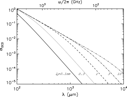
Figure 1: Absorption spectrum due to a Disordered Charge Distribution. The absorption coefficient $\alpha_{\rm DCD}$ is given in arbitrary units, normalized at $\lambda=100\,{\rm\mu m}$ and $l_{\rm c}=10\,nm$. The solid, dot, dash, dash-dot and dash-dot-dot lines correspond to $l_{\rm c}=0.1$, 0.3, 1, 3 and $10\,nm$ respectively, assuming a transverse sound velocity $\upsilon_{t}=3\cdot 10^{5}$ cm/s.

4.3 TLS Absorption

4.3.1 Phenomenological TLS Theory

At low temperatures, the thermal and dielectric properties of disordered solids (e.g. glasses and mixed crystals) show definite deviations from the predictions of the phonon theory developed for perfectly ordered crystals. Most of these phenomena can be described in the formalism of the so called Two Level Systems (TLS), which is the simplest model of tunneling states. In comparison to DCD it could be considered as a second approximation for the description of electromagnetic properties of solids linked to disordering. Vacancies unavoidable in disordered lattices produce in first approximation a possibility for chaotic distribution of some charges, which was considered in the previous section. This distribution is considered as frozen in the lattice due to the large height of barrier dividing vacancies in comparison with the available thermal energy. The TLS theory takes into account transitions of charges due to quantum tunneling possible at any temperature.

The TLS theory is the result of a macroscopic analysis of phenomena as opposed to an exact microscopic description. It is based on the hypothesis of a flat distribution of tunneling states with energy level differences sufficiently low with respect to the usual vibrational energy. The temperature dependance of two-level system properties results from deviations from the model of harmonic oscillator, which is a good approximation for the description of crystal lattice vibrations. The origin of TLS is vacancies in the lattice which gives the possibility, for atoms or groups of atoms, to have different equilibrium spatial configurations. As a result, the potential curve has at least a double-well form (DWP, see Fig. 2) in contrast to single-well potential (SWP) of harmonic oscillators in crystal without vacancies.

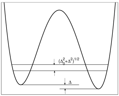
Figure 2: Asymmetric double-well potential. Ordinate is the potential energy. Abscissa is a coordinate in configuration space, in the simple case a rotation angle or a linear displacement of groups of atoms in the lattice. $\Delta$ is the value of potential asymmetry. The difference in energies of the lowest levels results from the asymmetry $\Delta$ and tunnel splitting $\Delta_{0}$.

In the TLS model described e.g. by (Phillips Phillips87 (1987)), the energy distribution of states is defined under the assumption that the asymmetry $\Delta$ of DWP and the height $V$ of the DWP potential barrier are stochastic values and their probability distribution can be assumed constant over a certain range of $V$ and $\Delta$ values. Like for the well known tunneling probability, the energy splitting $\Delta_{0}$ has an exponential dependence with barrier width $d$:

$$\Delta_{0}=\hbar\Omega\exp[-d(2mV)^{1/2}/\hbar],$$ (60)

where $\hbar\Omega=(E_{1}+E_{2})/2$ is the average energy of levels and $m$ is the effective mass. This exponential dependence along with the flat probability distributions of $\Delta$ and $V,$ leads to the 2-dimensional distribution

$$P(\Delta_{0},\Delta)=\overline{P}/\Delta_{0},$$ (61)

where $\overline{P}$ is a constant. The integral of $P$ over $\Delta_{0}$ does not diverge because the lowest $\Delta_{0}$ values are limited by the highest energy $V$ through Eq.(60).

The exact form of $P(\Delta_{0})$ in the vicinity of $\Delta_{0}^{\min}$ is not important in most cases because the corresponding energy ($\Delta_{0}^{\min}/k_{\rm\tiny B}\ll 0.01\,K$) are very far from values under consideration. A value of constant $\overline{P}$ is not defined by the TLS theory, it varies from one material to another, and can be regarded as a free parameter to be determined from experiments or observations.

In oder to better understand the TLS phenomenological approach, Kühn (Kuhn01 (2003)) built a microscopic model using the translational invariant Hamiltonian

$$H = \sum_{j}\frac{p_{j}^{2}}{2m}+U(\{u_{j}\}),$$

$$U = \frac{1}{4}\sum_{ij}J_{ij}(u_{i}-u_{j})^{2}+\frac{g}{2N}\sum_{ij}(u_{i}-u_{j})^{4},$$ (62)

where $p_{j}$ are impulses, $u_{j}$ are displacements of $j$-th atom from some reference points. The first term is a quadratic potential with random coefficients $J_{ij}$. The second term is a stabilizing quartic potential (not random) with a constant $g>0$ coefficient. The stochastically simulated coefficients $J_{ij}$ lead to disordered equilibrium arrangement of atoms. Disordered potential relief (Eq. 62) reproduces an ensemble of states both SWP and DWP, with a broad spectrum of barrier heights $V$ and asymmetries $\Delta$.

Some TLS effects associated with excited-state transitions of TLS could be brought to the fore in some laboratory experiments (FitzGerald et al.FitzGerald94 (1994) and Sievers et al. Sievers98 (1998)) on a number of mixed fluorite crystals and soda-lime silica glass. However these effects can only be seen in a narrow temperature range, roughly below 15K, before relaxation processes dominate at higher temperature. These effects will be incorporated to our model in a forthcoming paper. In the following, we restrict our consideration to the two lowest levels with energy difference $E=E_{2}-E_{1}=\sqrt{\Delta^{2}+\Delta_{0}^{2}}$.

As opposed to thermal properties, the TLS absorption spectrum depends not only on the TLS density of states distribution $P$ over energies $\Delta_{0}$, $\Delta$, but also on the values of the matrix elements of the dipole transitions between levels

$$\langle 1|\mu|2\rangle=\mu_{\rm b}\frac{\Delta_{0}}{E},$$ (63)

where $\mu$ is an electric dipole moment,

$$\mu_{\rm b}=\frac{1}{2}\frac{\partial\Delta}{\partial\xi},$$ (64)

where $\xi$ is the value of the electrical field.

The dipole moment $\mu_{\rm b}$ is the second TLS parameter, which characterizes its interaction with the electromagnetic field. For isotropic materials the square of dipole moment should be averaged over all directions as $\langle\mu_{\rm b}^{2}\rangle=\mu_{\rm b}^{2}/3$. Like the parameter $\overline{P}$ discussed above, the parameter $\mu_{\rm b}$ varies from one material to another, and can be regarded as a free parameter, to be determined by experiments or observations. In some experimental publications, values of the dipole moment are given, which are not corrected for the local field and orientation averaging, $\mu^{\prime}=\mu_{\rm b}(\epsilon^{\prime}+2)/3\sqrt{3}$.

The TLS absorption spectrum shape can be obtained by solving the Bloch equations which describe the interaction of TLS with electromagnetic wave and lattice oscillations. The latter interaction is described by the third material dependent parameter of TLS theory, i.e. the elastic dipole moment given by :

$$\gamma_{\rm e}=\frac{1}{2}\frac{\partial\Delta}{\partial e},$$ (65)

where $e$ is the value of the strain field. The order of magnitude of $\mu_{\rm b}$ and $\gamma_{\rm e}$ is about 1 D and 1 eV, respectively.

The solution of general equations for the TLS absorption can be described as a result of two different contributions: an absorption which has a resonant character and an attenuation which has the typical form of a relaxation. In practice it is convenient to treat these processes separately. Bösch Bosch78 (1978) explained his experimental results considering three processes: resonant tunneling , relaxation due to phonon-assisted tunneling, relaxation due to phonon-assisted hoping over the potential barrier. In the next sections, we will discuss each of them in more details.

4.3.2 Resonant absorption

The resonant absorption of a photon of energy $\hbar\omega$ concerns only those TLS characterized by the splitting energy $E_{2}-E_{1}=\hbar\omega$ . Let $N(\omega)$ be the density per unit frequency of those TLS, and $N_{1}(\omega)$ and $N_{2}(\omega)$ the densities per unit frequency of those TLS which are in the state of energy $E_{1}$ and $E_{2}$ respectively. Of course these densities are strongly temperature dependent, but in the TLS model only the two lower levels are considered and it is assumed that $N=N_{1}+N_{2}$.

The resonant tunneling absorption then takes the form

$$\alpha_{\rm res}=\frac{\hbar\omega}{c\sqrt{\epsilon^{\prime}}}B_{12}\Big{(}\frac{\epsilon^{\prime}+2}{3}\Big{)}^{2}(N_{1}-N_{2}),$$ (66)

where $B_{12}$ is the Einstein coefficient for absorption,

$$B_{12}=\frac{4\pi^{2}\langle 1|\mu|2\rangle^{2}}{3\hbar^{2}}.$$

The population of the levels under the thermal equilibrium hypothesis gives

$$N_{1}-N_{2}=N(\omega)\tanh(\hbar\omega/2k_{\rm\tiny B}T),$$

and taking into account that $E=\hbar\omega$

$$\alpha_{\rm res}=\frac{4\pi^{2}\omega}{3c\sqrt{\epsilon^{\prime}}}\Big{(}\frac{\epsilon^{\prime}+2}{3}\Big{)}^{2}\tanh(\hbar\omega/2k_{\rm\tiny B}T)\ G(\omega),$$ (67)

where

$$G(\omega)=\frac{\overline{P}\mu_{\rm b}^{2}}{(\hbar\omega)^{2}}\int_{0}^{\hbar\omega}\frac{p_{\rm\tiny G}(\Delta_{0})\Delta_{0}\mathrm{d}\Delta_{0}}{\sqrt{1-(\Delta_{0}/\hbar\omega)^{2}}}.$$ (68)

Equation (67) was derived in the work of Hubbard et al. (Hubbard03 (2003)), the term $G(\omega)$ is the so called Optical Density Of States (ODOS) and can be determined from laboratory spectroscopy.

The coefficient $p_{\rm\tiny G}(\Delta_{0})\la 1$ we introduced in Eq. (68) to describe deviation of $P(\Delta_{0})$ from Eq. (61) at large $\Delta_{0}$. To avoid confusion in this work we will not change definitions of variables where it is possible, preferring transformation of the original equations taken from different sources.

In the TLS theory, confirmed by low-temperature measurements of thermal properties, $p_{\rm\tiny G}=1$ for energies smaller than $10^{-3}$ eV. If $p_{\rm\tiny G}=1$ for all $Delta_{0}$, Eq. (68) gives $G(\omega)=\overline{P}\mu_{\rm b}^{2}$=const. Expression for the TLS resonant tunneling absorption, corresponding to $p_{\rm\tiny G}=1$, was used by Bösch (Bosch78 (1978)) and Schickfus et al. (Schickfus75 (1975), Schickfus76 (1976)):

$$\alpha_{\rm res}=\frac{4\pi^{2}\overline{P}\,\mu^{\prime 2}}{c\sqrt{\epsilon^{\prime}}}\omega\;\tanh(\hbar\omega/2k_{\rm\tiny B}T).$$ (69)

The frequency independent ODOS was found to be in satisfactory agreement with experiments for wavenumbers $\omega/2\pi c<$12 cm^-1. Its measured values ($\overline{P}\mu_{\rm b}^{2}$) are given in Table 1. Assuming $\mu^{\prime}=1D$, the density of states is $\overline{P}=0.9\cdot 10^{33}$ erg^-1 cm^-3 for soda-lime-silica glass.

More accurate spectroscopic measurements in wide spectral regions show a definite drop of $G(\omega)$ to zero within the error level, for $\omega$ higher than some frequency $\omega_{\rm m}$. Agladze & Sievers (Agladze98 (1998)) measured a profile with a cut-off at 20 cm^-1 in high density amorphous phase ices of H₂O and D₂O. Fitzgerald, Sievers & Campbell (2001a ) detected a sharp cut-off in fluoride mixed crystal spectra, with wavenumber $\omega_{\rm m}/2\pi c=$13 cm^-1. Hubbard et al. (Hubbard03 (2003)) observed a shallow cut-off at $\omega_{\rm m}/2\pi c=$15 cm^-1, 9 cm^-1 and 6 cm^-1 for the soda lime silica, the SiO₂ and the germanium glasses, respectively.

Hubbard et al. (Hubbard03 (2003)) suggested that the distribution $P(\Delta_{0},\Delta)$ (Eq. 61) has a cut-off at energy $E_{\rm m}=\hbar\omega_{\rm m}$. In our Eq. (68) it corresponds to $p_{\rm\tiny G}(\Delta_{0})$ in the form of a step function

$$p_{\rm\tiny G}(\Delta_{0})=\left\{\begin{array}[]{ll}1&\textrm{for $\Delta_{0}<E_{\rm m}$}\\ 0&\textrm{for $\Delta_{0}>E_{\rm m}$.}\end{array}\right.$$ (70)

Under this assumption, Hubbard et al. (Hubbard03 (2003)) calculated a frequency dependent expression for the ODOS by means of integration of distribution function equivalent to Eq. (68). For our consideration it is convenient to write it in the form

$$G(\omega)=g(\omega/\omega_{\rm m})\overline{P}\mu_{\rm b}^{2}.$$ (71)

The ODOS of (Hubbard et al. Hubbard03 (2003)) is described by the following function :

$$g(\omega/\omega_{\rm m})=\left\{\begin{array}[]{ll}1&\textrm{for $\omega/\omega_{\rm m}\leq 1$}\\ 1-\sqrt{1-(\omega/\omega_{\rm m})^{-2}}&\textrm{for $\omega/\omega_{\rm m}>1$}.\end{array}\right.$$ (72)

However, the spectra corresponding to the ODOS proposed by Hubbard et al. (Hubbard03 (2003)) (Eq. 72) exhibits a prominent break which was not observed in laboratory spectra of noncrystaline materials and has not been observed in spectra of astronomical dust emission.

We suggest that the cut-off of the distribution function should be complemented by a continuity condition and therefore continuity of $p_{\rm\tiny G}(\Delta_{0})$. The simplest form of continuous function for $p_{\rm\tiny G}(\Delta_{0})$ is considered in Appendix A and leads to the following a shape of the ODOS

$$g(x)=\left\{\begin{array}[]{ll}1+x^{2}g_{1}(x)&\mathrm{for}\ x<1,\\ 1+x^{2}g_{1}(x)-g_{2}(x)\sqrt{1-x^{-2}}&\mathrm{for}\ x>1.\end{array}\right.$$ (73)

where $x=\omega/\omega_{\rm m}$, polynoms $g_{1}(x),\ g_{2}(x)$ are defined in Appendix by Eq. (104) and Eq. (105).

This ODOS function has no break at $\omega=\omega_{\rm m}$, it is in better agreement with laboratory measurements of amorhous materials. It is also in full agreement with TLS theory at $\omega\ll\omega_{\rm m}$. For this reason it will be used in the calculations of Sect. 5.

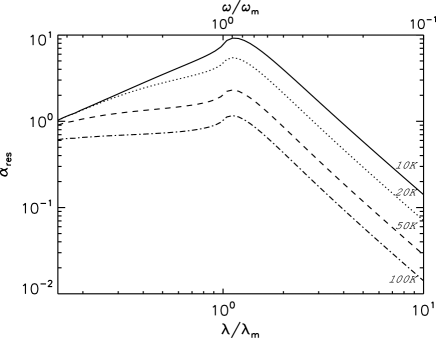
Figure 3: Absorption spectrum due to resonant tunneling in Two Level Systems. The absorption coefficient is given in relative units normalized at $\lambda=100\,{\rm\mu m}$ and $T=10\,K$. The abscissa axis is normalized to the cut-off wavelength of the Optical Density of States $\lambda_{\rm m}=700\,\,{\rm\mu m}$ (see text). The solid, dot, dash and dash-dot lines correspond to $T=10$, 20, 50 and $100\,K$ respectively. The various curves can be scaled using the simple relation $\lambda_{\rm m}T$=const. In the low frequency wings, curves scale as $\alpha\sim\omega^{2}/T$.

4.4 Relaxation processes

Direct consideration of the relaxation processes permits to evaluate the nonresonant part of TLS absorption spectra through analysis of the mechanism of the TLS level population relaxations after some deviation from equilibrium. The relaxation time constant $\tau$ is determined by the rate ($\tau^{-1}$) of transitions between levels, in which transitions due to intensive interactions with the lattice thermal oscillations (phonons) dominate.

The rate of the TLS transitions as a result of strain field generated by thermal fluctuations in a lattice was evaluated by Phillips (Phillips72 (1972)).

$$\tau(\Delta_{0},E)\ ^{-1}=\tau_{1}^{-1}\ \Delta_{0}^{2}\ E^{-2},$$ (74)

where

$$\tau_{1}=a\ E^{-3}\tanh(E/2k_{\rm\tiny B}T)$$ (75)

and

$$a=\pi\upsilon_{t}^{5}\rho\hbar^{4}\gamma_{e}^{-2}$$ (76)

is a material constant. Parameters included in Eq. (76) were already described above.

Phillips (Phillips72 (1972)) calculated also an equilibrium value of the TLS dipole moment $\overline{\mu}$ and therefore the resulting susceptibility $\chi(\omega)$ in the form of a Debye spectrum (Eq.  28):

$$\chi_{0}^{\prime\prime}(\omega)=\frac{\mu_{\rm b}^{2}}{3k_{\rm\tiny B}T}\frac{\Delta^{2}}{E^{2}}\textrm{sech}^{2}\Big{(}\frac{E}{2k_{\rm\tiny B}T}\Big{)}\frac{\omega\tau}{1+(\omega\tau)^{2}}$$ (77)

The rate of tunneling relaxation (Eq. 74) is proportional to the tunneling probability, so it does not take into account direct transitions in TLS which energy is higher than the barrier height. This transition rate is proportional to the number of phonons with such energy, which should follow a Boltzman distribution and depends on temperature and on the energy barrier height $V$. In glasses with $V/k_{\rm\tiny B}\ga 500$ K the time of hopping relaxation $\tau$ varies with $T<100$ K in accordance with the Arrhenius relation (Hunklinger & Schickfus Hunklinger81 (1981)).

$$\tau=\tau_{0}\ \exp(V/k_{\rm\tiny B}T)$$ (78)

with $\tau_{0}\approx 10^{-13}$ s (fused silica).

Experimental values of $V$ and $\tau_{0}$ were determined using the temperature dependence of the position of the spectrum maximum ($\omega=\tau^{-1}$, see Eq.  77). The distribution of TLS on $V$ leads to the broadening of the corresponding spectrum, sometimes preventing definite detection of its maximum. The measurement of the spectrum broadening permits to evaluate the width and shape of the TLS distribution on $V$. In practice experimentalists often use the shape of a truncated Gaussian probability distribution to fit the energy distribution of TLS.

$$P(V)=C_{V}\ p_{\rm\tiny V}(V),$$ (79)

where

$$p_{\rm\tiny V}(V)=\left\{\begin{array}[]{ll}\exp(-(V-V_{\rm m})^{2}/V_{0}^{2})&\textrm{ for }V>V_{\min},\\ 0&\textrm{ for }V<V_{\min},\end{array}\right.$$ (80)

where $C_{V}$ is the usual normalization coefficient (Eq. 111) depending on $V_{\rm m},\ V_{0},\ V_{\min}$, which are parameters of the distribution shape. An example of measured numerical values of these parameters is given in Table 1.

Starting from known distribution of TLS on energies $E,\ \Delta_{0},\ V$ and spectrum (Eq. 77) for fixed values of $E,\ \Delta_{0},\ V$ one can synthesize a final relaxation spectrum. The integrated spectra are considered in the following sections.

4.4.1 Tunneling relaxation

The absorption spectrum due to phonon-assisted tunneling relaxation can be obtained by integration of Eq. (77) on $E$ and $\Delta_{0}$. The expression for this was provided by Fitzgerald, Campbell & Sievers.(2001b )

$$\alpha_{\rm phon}=A\cdot\omega\cdot F(\omega,T),$$ (81)

where

$$A=\frac{\overline{P}\mu_{\rm b}^{2}}{3c\sqrt{\epsilon}}\Big{(}\frac{\epsilon^{\prime}+2}{3}\Big{)}^{2}$$ (82)

is a material constant and :

$$F(\omega,T) = \frac{1}{2k_{\rm\tiny B}T}\int^{\infty}_{0}\int^{\infty}_{\tau_{1}}\sqrt{1-\frac{\tau_{1}}{\tau}}\ \textrm{sech}^{2}\Big{(}\frac{E}{2k_{\rm\tiny B}T}\Big{)}\frac{\omega\ \mathrm{d}\tau\ \mathrm{d}E}{1+\omega^{2}\tau^{2}},$$

with $\tau_{1}$ given by Eq. (75). A change of variables made using relation between $\Delta_{0}$ and $\tau$ for integral calculation.

Another, simplified equation describing tunneling relaxation absorption was used by Jackle (Jackle72 (1972)) and by Bösch (Bosch78 (1978))

$$\alpha_{\rm phon} = A\int^{\infty}_{0}\frac{\mathrm{d}E}{2k_{\rm\tiny B}T}\textrm{sech}^{2}\Big{(}\frac{E}{2k_{\rm\tiny B}T}\Big{)}\frac{\omega^{2}\tau_{1}}{1+\omega^{2}\tau_{1}^{2}},$$ (83)

where $\tau_{1}$ is given by Eq. (75), parameters $A$ and $a$ (in Eq. 75) are to be defined from experiments. The use of Eq. (83) is equivalent to evaluating the integral in Eq. (77) substituting values by that for a symmetric DWP $\Delta$=0. Formally it is equivalent to replacing $\sqrt{1-\tau_{1}/\tau}$ by $\tau_{1}\delta(\tau-\tau_{1})$. Our evaluation shows large inaccuracy in this procedure for values of absorption. For details see Appendix B.

However, this approach gives satisfactory accuracy for time constant evaluation linked to parameter $a$. For soda-silica glass (Bösch Bosch78 (1978)) $a=4.2\cdot 10^{-56}$ erg³s. It corresponds to $\gamma_{e}=0.5$ eV (see Table 1).

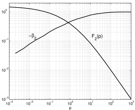
Figure 4: The function $F_{\rm phon}(p)$ (solid line) and the exponent of its slope $\beta_{2}=d\ln F_{\rm phon}/d\ln p$ (dotted line) plotted as a function of the parameter $p=a_{\rm phon}\omega/(2k_{\rm\tiny B}T)^{3}$ (see text). The spectral index of phonon absorption $\beta_{\rm phon}$ is related to $\beta_{2}$ as $\beta=1+\beta_{2}$ and ranges from $\beta_{\rm phon}=1$ at low frequencies (low p values) to $\beta_{\rm phon}=2$ at high frequencies (high p values). The temperature dependence $p(T)$ generates a shift of the absorption spectra along the frequency axis.

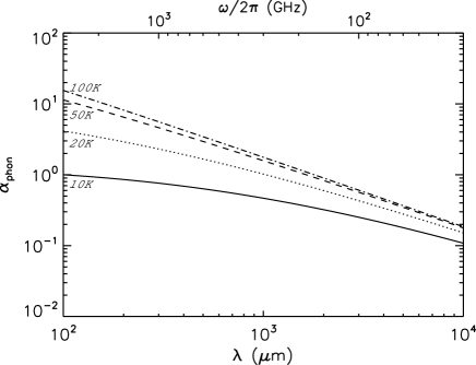
Figure 5: Spectra of absorption due to tunneling relaxation $\alpha_{\rm phon}$ in the FIR/mm. The absorption coefficient is given in arbitrary units, normalized at $\lambda=100\,{\rm\mu m}$ and $T=10\,K$. Line styles are the same as in Fig. 3

The full equation (4.4.1) for calculation of phonon relaxation spectra can be simplified without loss of accuracy. We made it using a function of one argument $F_{\rm phon}(p)$ instead of a function of two arguments $F(\omega,T)$ in Eq. (81). We introduce the intermediate parameter $p(\omega,T)=a\omega/(2k_{\rm\tiny B}T)^{3}$. This permits to use a one-dimensional grid of argument, efficiently reducing computing time. The use of interpolation in precalculated values (Table 3 in Appendix) make use of this function as fast as a standard one.

Therefore an accurate and relatively simple equation for tunneling relaxation spectrum is

$$\alpha_{\rm phon}=A\cdot\omega\cdot F_{\rm phon}(a\omega(2k_{\rm\tiny B}T)^{-3}),$$ (84)

where $A$ (Eq. 82) is a material constant and the function $F_{\rm phon}$ is given by

$$F_{\rm phon}(p) = \int^{1}_{0}\int^{\pi/2}_{x_{1}}\sqrt{1-\frac{\tan x_{1}}{\tan x}}\ \mathrm{d}x\mathrm{d}y,$$ (85)

$$x_{1} = \arctan(p\ y\textrm{ arcth}^{-3}y).$$ (86)

A plot of function $F_{\rm phon}(p)$ is shown on Fig. 4.

The absorption spectrum for tunneling relaxation is temperature dependent in accordance with Eq. (81). As opposed to resonant absorption, the tunneling relaxation absorption increases with temperature, as shown on Fig. 5

4.4.2 Hopping relaxation

The expression for the absorption spectrum due to hopping relaxation can be obtained by integrating Phillip’s equation (77) over a Gaussian distribution of barrier height $p_{\rm\tiny V}(V)$ given in Eq. (80) :

$$\alpha_{\rm hop}=B_{\rm hop}(T)\ \omega\ \int^{\infty}_{0}\frac{\omega\tau}{1+\omega^{2}\tau^{2}}P(V)\ \mathrm{d}V,$$ (87)

where $\tau=\tau_{0}\exp(V/k_{\rm\tiny B}T)$ and the coefficient $B_{\rm hop}(T)$ does not depend on $\omega$.

Examples of spectra described by Eq. (87) are shown on Fig. 6. It is known from general principles that the asymptotic behavior of $\epsilon(\omega)$ when $\omega\rightarrow 0$ leads to $\alpha(\omega)\sim\omega^{2}$ (spectral index $\beta$=2). Figure 6 shows that this region begins at $f<10$ MHz for $T$= 100 K and at $f<100$ Hz for $T<50\,K$.

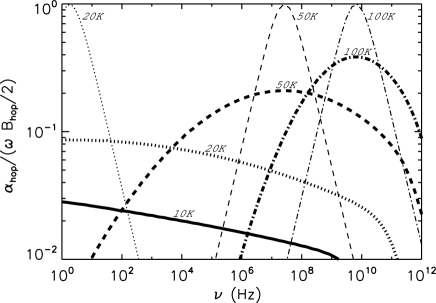
Figure 6: Hopping relaxation absorption spectra in the frequency range from 1 Hz to $1$ THz. The ratio of the absorption coefficient $\alpha_{\rm hop}$ to the parameter $\omega B_{\rm hop}/2$ is plotted to show the whole spectrum at comparable scales and to evidence variations of the peak position with temperature. The curves are computed using a barrier height of $V_{\rm m}/k_{\rm\tiny B}$=550 K (see Tab. 1). Line styles are the same as in Fig. 3. Thin curves correspond to unbroadened spectra with $V_{0}\ll V_{\rm m}$. Thick curves correspond to $V_{0}/k_{\rm\tiny B}=$410 K.

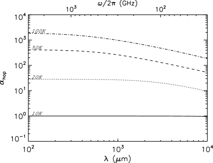
Figure 7: Spectra of absorption due to hopping relaxation $\alpha_{\rm hop}$ in the FIR/mm. The absorption coefficient is given in arbitrary units, normalized at $\lambda=100\,{\rm\mu m}$ and $T=10\,K$. Line styles are the same as in Fig. 3 In this relatively narrow spectral region, the behavior of the curves is in agreement with the approximation of Eq. (89).

At high frequencies (beginning from mm-wave region) the spectra shown on Fig. 7 are determined by the low energy part of the barrier height distribution. It can be approximated by

$$\alpha_{\rm hop}\approx B_{\rm hop}(T)\omega P_{\min}\int^{\infty}_{V_{\min}}\frac{\omega\tau}{1+\omega^{2}\tau^{2}}\ \mathrm{d}V,$$ (88)

where $P_{\min}=P(V_{\min})$, and therefore

$$\alpha_{\rm hop}\approx B_{\rm hop}(T)\omega P_{\min}k_{\rm\tiny B}T\ \arctan\Big{(}\frac{e^{-V_{\min}/k_{\rm\tiny B}T}}{\omega\tau_{0}}\Big{)}.$$ (89)

For spectra on Fig. 7, a value of $P_{\min}$ corresponds to $P_{\min}\,k_{\rm\tiny B}=$$\exp[-(V_{\min}-V_{\rm m})^{2}/V_{0}^{2}]/V_{0}\sqrt{\pi}$ = 3.11$\cdot 10^{-4}$ K^-1.

Bösch (Bosch78 (1978)) used an approximated expression $B_{\rm hop}=h_{r}/T$, where $h_{r}$ is a constant. The approximation used by Fitzgerald et al. (2001b ) gives $B_{\rm hop}=2\pi\mu^{2}/3c\sqrt{\epsilon^{\prime}}$ which is a material constant. In Annex D, we derive a more accurate approximation which gives

$$B_{\rm hop}(T)=\frac{8\pi}{3c\sqrt{\epsilon^{\prime}}}\frac{(\epsilon^{\prime}+2)^{2}}{9}\overline{P}\mu_{\rm b}^{2}(c_{\Delta}+\ln T),$$ (90)

where T is in Kelvin and material constant $c_{\Delta}$ is given by

$$c_{\Delta}=\ln\frac{k_{\rm\tiny B}}{\Delta_{0}^{\min}}+\ln 4-1+\int_{0}^{1}\ln{\rm arcth}\ x\ \mathrm{d}x$$ (91)

in accordance with Eq. (90) and (113). $c_{\Delta}$ is therefore an additional parameter of tunneling states. Its value corresponds to tunnel splitting in low $\Delta$ region where tunneling state density distribution becomes significantly less than that of Eq. (61). The TLS theory was proved to apply in low temperature experiments at $T$ down to 2 mK (Phillips Phillips87 (1987)), therefore $\Delta_{0}^{\min}/k_{\rm\tiny B}<2\cdot 10^{-3}$ K and $c_{\Delta}$ should verify $c_{\Delta}\ga 5.8$. The dependence of $B_{\rm hop}(T)$ is relatively weak and a tenfold variation in $T$ from 10 K to 100 K leads to variation of $B_{\rm hop}(T)$ less than $30\%$.

A difference in temperature dependence of considered approximations is significant, especially for absorption calculations over a wide range of temperatures. It does not manifest itself when fitting laboratory data over a limited region of temperature, leading only to a biased value of a parameter $A$. The main temperature dependence of $\alpha_{\rm hop}$ is defined by exponential dependence of $\tau$ on $T$ (Eq. 78).

In the work of Bösch (Bosch78 (1978)), Fitzgerald et al. (2001b ) and others, a comparison between experimental and calculated temperature dependancies was performed . It showed that relaxation processes should be taken into account for temperatures $T\ga 10\,K$. At these temperatures, relaxation dominates over resonant tunneling. Hopping relaxation becomes significant at $T$ about 25 K and dominates at higher temperature. This tendency has a general character, and shows a similar behavior for substances as different as fluoride mixed crystals and silica glasses.

5 Model of the dust FIR/mm emission

The theoretical considerations given in Sect. 4 provide the formalism for calculations of dust emissivity in the far-infrared and millimeter-wave region and can be gathered into a new model for explaining the astronomical emission in this spectral range. So far, modeling the astronomical dust emission spectra in this spectral range has been performed on purely phenomenological grounds with little connection to solid states physics. Unlike previous models, the new approach proposed here does not assume that dust is composed of crystalline material, but instead uses for the first time theoretical results applicable to disordered materials which are likely to compose astronomical dust particles.

5.1 Model description

The mass absorption coefficient of dust entering Eq. 1 can be expressed as

$$\kappa_{\rm dust}=\kappa_{\rm\tiny IR}+\kappa_{\rm\tiny DCD}+\kappa_{\rm\tiny TLS}.$$ (92)

The first term $\kappa_{\rm\tiny IR}$ includes the opacity in infrared bands and other relatively short-wave absorption processes. References to dust models describing $\kappa_{\rm\tiny IR}$ are given in Sect. 1. IR bands in the dust spectrum are linked to the optical modes of lattice oscillations, like bending vibration bands of interatomic bonds such as O-Si-O or H-O-H. As was shown in the previous sections, the long wavelengths wing of infrared bands is relatively weak in the FIR/mm. Our model does not provide a new description of these processes and is complementary to IR models. While $\kappa_{\rm\tiny IR}$ depends mainly on the chemical composition of dust, the following terms $\kappa_{\rm\tiny DCD}$ and $\kappa_{\rm\tiny TLS}$ are linked to the disordered structure of the grain material and are largely independent of the dust chemical composition.

As described in Sect. 4, $\kappa_{\rm\tiny DCD}$ and $\kappa_{\rm\tiny TLS}$ are linked to the existence of disorder in the structure of the grain material. Given the fast decrease of $\kappa_{\rm\tiny IR}$ with wavelength, these effects are likely to dominate absorption in the FIR/mm. Disordered media absorption takes place in all substances excluding perfect crystals. Amorphous dust as well as partially ordered or dirty crystalline dust can therefore be described by the model.

The first term, $\kappa_{\rm\tiny DCD}$ corresponds to disordered charge absorption described in Sect. 4.2. It is temperature independent. The second term, $\kappa_{\rm\tiny TLS}$ is connected with transition of charges in a lattice between vacant potential minima due to tunneling or thermal activation (Sect. 4.3). This term displays a specific spectrum of absorption over a wide range of frequencies $\omega/2\pi$, from about 1 Hz to about $1$ THz. It includes three components designated in the model as resonant ($\kappa_{\rm res}$), tunneling relaxation ($\kappa_{\rm phon}$), and hopping relaxation ($\kappa_{\rm hop}$) respectively :

$$\kappa_{\rm\tiny TLS}(\omega,T)=\kappa_{\rm res}(\omega,T)+\kappa_{\rm phon}(\omega,T)+\kappa_{\rm hop}(\omega,T).$$ (93)

Spectral index of $\kappa_{\rm\tiny TLS}$ significantly deviates from $\beta=2$ and depends on temperature. Resonant opacity $\kappa_{\rm res}$ decreases with $T$, relaxation opacity $\kappa_{\rm phon}$ and $\kappa_{\rm hop}$ rises with $T$.

The various opacities of the model can be summarized as,

$$\kappa_{\rm\tiny DCD}(\omega) = K_{\rm\tiny DCD}\omega^{2}\left[1-\left(1+\omega^{2}/\omega_{c}^{2}\right)^{-2}\right],$$ (94)

$$\kappa_{\rm res}(\omega,T) = K_{\rm\tiny TLS}\omega\ g_{\rm res}\left(\frac{\omega}{\omega_{\rm m}}\right)\tanh\left(\frac{\hbar\omega}{2kT}\right),$$ (95)

$$\kappa_{\rm phon}(\omega,T) = \frac{1}{4\pi^{2}}K_{\rm\tiny TLS}\ \omega\ F_{\rm phon}(a_{\rm phon}\omega T^{-3}),$$ (96)

$$\kappa_{\rm hop}(\omega,T) = \frac{2}{\pi}K_{\rm\tiny TLS}\omega(c_{\Delta}+\ln T)\int^{\infty}_{V_{\min}}\frac{\omega\tau(V,T)P(V)\mathrm{d}V}{1+\omega^{2}\tau^{2}(V,T)},$$ (97)

where $\tau(V,T)=\tau_{0}\ \exp(V/k_{\rm\tiny B}T)$.

The amplitude factors for the DCD and TLS terms can be expressed with respect to material properties as follows:

$$K_{\rm\tiny DCD} = \overline{q^{2}_{\rm m}}\ (3\upsilon_{t}^{3}c\rho)^{-1},$$ (98)

$$K_{\rm\tiny TLS} = \frac{4}{3}\pi^{2}\overline{P}\mu_{\rm b}^{2}\ (c\rho)^{-1},$$ (99)

$$a_{\rm phon} = \pi\gamma_{\rm e}^{-2}\upsilon_{t}^{5}\rho\hbar^{4}(2k_{\rm\tiny B})^{-3}.$$ (100)

The function $g_{\rm res}$ is the normalized ODOS spectrum given by Eq. (73). The function $F_{\rm rel}$ is defined by Eq. (107) and can be calculated interpolating Eq. (109) using precalculated values in Table 3 of the Appendix.

The Gaussian probability distribution function of the TLS potential barrier height $P(V)$ is defined by Eq. (80) with parameters $V_{\rm m}$, $V_{0}$ and $V_{\min}$.

$K_{\rm\tiny DCD}$ and $K_{\rm\tiny TLS}$ define the amplitude scale of $\kappa_{\rm\tiny DCD}$ and $\kappa_{\rm\tiny TLS}$. Parameters $\omega_{c}$, $\omega_{\rm m}$, $a_{\rm phon}$, $\tau_{o}$ define the scale of $\kappa_{\rm\tiny DCD},\ \kappa_{\rm res},\ \kappa_{\rm phon},\ \kappa_{\rm hop}$, respectively, along the $\omega$ axis.

The numerical values and units of the various parameters entering the model are given in Tab. 2. They set the frequency and temperature dependence of the model.

It is important to note that the values proposed here only give an order of magnitude for the parameters, and are derived only from laboratory measurements (Sect. 3.2.3 and 4) or theoretical expectations. They provide reference values only. They are not tuned to reproduce observed astronomical spectra. Derivation of the parameter values to be used for astronomical purposes will be derived in a forthcoming paper.

Table 2: Parameter values.

parameter	value	unit
$K_{\rm\tiny DCD}$†	$1.2\cdot 10^{-24}$	${\rm cm^{2}g^{-1}s}^{2}$
$K_{\rm\tiny TLS}$†	$1.5\cdot 10^{-13}$	${\rm cm^{2}g^{-1}s}$
$\omega_{c}$‡	$3.10^{12}$	${\rm s}^{-1}$
$\omega_{\rm m}$♭	$2.7\cdot 10^{12}$	${\rm s}^{-1}$
$a_{\rm phon}$†	$5.3\cdot 10^{-10}$	${\rm K^{3}s}$
$\tau_{o}$ ⋆⋆	$10^{-13}$	${\rm s}$
$V_{\rm m}$ ⋄	$7.6\cdot 10^{-14}$	${\rm erg}$
$V_{0}$ ⋄	$5.7\cdot 10^{-14}$	${\rm erg}$
$V_{min}$ ⋄	$6.9\cdot 10^{-15}$	${\rm erg}$
$c_{\Delta}$ ⋆	$5.8$

^† values calculated using Eq. (98-100) and the following approximate mean values : $\upsilon_{t}=3\cdot 10^{5}$ cm/s, $\rho$ = 3 g/cm³, $\overline{P}\mu_{\rm b}^{2}=10^{-3}$, $\gamma_{e}$ = 1 eV, $\overline{q^{2}_{\rm m}}=e^{2}/m_{o}$, where $e$ is the electron charge and $m_{o}$ is the mass of the Oxygen atom.
^‡ using $l_{c}=\upsilon_{t}/\omega_{c}$=1 nm (see Tab. 1)
^♭ corresponds to $2\pi c/\omega_{\rm m}$=0.7 mm (see Sect. 4.3.2)
^⋄ from Table 1
^⋆⋆ $\tau_{o}$ from Sect. 4.4
^⋆ evaluated from Sect. 4.4.2.

5.2 Model applicability

5.2.1 Wavelength range of validity

The model presented here applies to FIR to millimeter emission from amorphous materials. In the astronomical context, it should be used to describe the emission of large dust grains which usually dominate the observed spectra in the FIR/mm. In principle, it should also apply to the emission from amorphous very small 3-D particles which emission usually dominates the mid-IR region of astronomical spectra.

The DCD component is valid only in the frequency range dominated by acoustic oscillations. Towards high frequencies the corresponding limit is set where the sound wavelength is of the order of the interatomic distances $d$. For silicates this corresponds to an electromagnetic wavelength $\lambda_{d}\simeq 10\,{\rm\mu m}$. At shorter wavelengths IR models should be used. Towards the long wavelengths, the validity is limited to $\omega\leq\omega_{a}$ with

$$\omega_{a}\approx\pi\upsilon_{t}/a,$$ (101)

where $\upsilon_{t}$ is the transverse sound velocity and $a$ is the grain size. The DCD model should therefore be valid for all wavelengths below $\lambda_{a}=3\,mm$ for the range of sizes usually assumed for the BG component (e.g. $15-110\,nm$ in Désert et al. Desert90 (1990)), using $\upsilon_{t}=3\,10^{5}\,cm/s$. Application of this part of the model to small transiently heated dust particles in the long wavelength range should therefore be handled with care.

The TLS part of the model is in principle not limited to a given spectral range.

5.2.2 Applicability in dust models

In general, modeling FIR/mm dust emission from an interstellar source be seen as a three-step process. The first step is to select the materials which constitute the grains, and specify the optical properties (complex dielectric constants or refractive index, or opacities) of the selected materials. The second step is to chose, for each dust component, a distribution of size, shape, composite structure, orientation with respect to the direction of the incoming radiation field, in order to calculate extinction, absorption and diffusion using Mie or some multipole approximation method. The third step is to specify the dust density and radiation field distributions, and to include radiative transfer to calculate the dust emission on a given line of sight. The model presented here concerns the first step of this dust emission modeling only.

The equations proposed in Sect. 5 do not include the local field correction factor given in Eq. (15). They are valid for spherical or quasi-spherical particles. Any possible effect due to anisotropic shapes, such as a polarized emission by grains for example, is beyond the scope of this paper, and refers to the second step of modeling.

The model equations do not depend on macroscopic values of the dielectric constant and average density. All the parameters involved in the model have a local, microscopic meaning. Therefore the derived emissivities are defined by the total mass of dust, and do not depend on the porosity of the grains. The model should therefore be equally valid for fluffy and for bulk grains.

It is important to note that unlike standard modeling, our model shows that it is not sufficient for the first modeling step to select from databank some complex dielectric constants $\epsilon(\omega,T)$ obtained for bulk mineral samples of chemical composition corresponding to interstellar element abundancies. First, the particle size should be taken into account. Indeed, if the opacity (mass emissivity) of dust (Eq. 8) does not depend on particle size for a given dieletric constant $\epsilon(\omega)$, the dieletric constant$\epsilon(\omega)$ itself is size dependent, as shown in Sect. 5.1. Second, both DCD and TLS processes are more sensitive to the degree and the type of disorder in a given material, than to the exact chemical composition of the grain.

5.3 Temperature and frequency dust opacity behavior

In the general case, the model can produce a wide variety of spectral shapes, ranging from a ”classical” spectrum $\beta$=2 when only DCD is taken into account ($K_{TLS}=0$) and the correlation length caracterizing DCD is assumed infinite ($\omega_{c}$=0) to spectra with much flatter behaviors when TLS effects are included, with mean spectral index values $\beta$ over the whole FIR/mm range close to one at high dust temperatures. Some extreme cases even include the possibility of having $\beta<0$ or $\beta>2$ over some limited regions of the spectrum, due to the influence of the resonant TLS absorption and to the DCD cut-off respectively.

However, the model generates a ”typical emission profile” when a correlation length of nanometric scale is assumed, and when the TLS effects are expected and taken into account. This emission profile presents some interesting characteristic deviations compared to the commonly adopted profile (a modified black-body type emission characterized by a constant spectral index $\beta$=2). To illustrate this fact, we show on Fig. 8 the dust opacity spectrum including both the DCD and TLS components ($\kappa_{\rm dust}=+\kappa_{\rm\tiny DCD}+\kappa_{\rm\tiny TLS}$), calculated using Eq. (94-97) and adopting the parameter values given in Tab. 2. First, the slope of the dust opacity versus wavelength, and consequently the spectral index, are no longer constant over the whole FIR/mm spectral range. As the temperature increases, it begins to deviate in the longest wavelength range, starting from a local spectral index values higher than $\beta$=2 around T=10K, towards lower values down to around $\beta$=1. Second, as the temperature increases more, this spectral behavior propagates towards the short wavelengths of the FIR/mm range. It is remarkable that only with model parameter values referenced in the solid state physics literature, the temperature-dependent spectral behavior of the modeled dust opacity is in qualitative agreement both with laboratory data in that temperature range (Sect. 3.2.2 and 3.2.3).

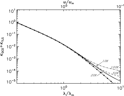
Figure 8: Total dust opacity spectra $\kappa_{\rm\tiny DCD}+\kappa_{\rm\tiny TLS}$. The spectra are given in arbitrary units, normalized at $\lambda=100\,{\rm\mu m}$ and $T=10\,K$. The dash-dot-dot line shows the temperature independant DCD dust opacity alone computed for $l_{\rm c}=1\,nm$. Line styles for the temperature dependant total effect are the same as in Fig. 3.

For each individual components of the model, the temperature and frequency behaviors have been described in Sect. 4. The DCD opacity is temperature independent and shows a quadratic frequency behavior ($\kappa_{\rm\tiny DCD}\sim\omega^{2}$) for high frequencies and drops dramatically ($\omega<\omega_{c}$) at lower frequencies. The transition between the two regimes is set by the value of the correlation frequency ($\omega_{c}$), or equivalently the correlation length of the charge distribution in the grain material. We point out that, although the transition between these two regimes is very smooth, this distinctive behavior opens the possibility to measure the correlation length from astronomical emission spectra. Note that the DCD effect is the only one with such a rapid fall-off of the absorption with wavelength, which seems to be measured toward some astronomical sources which exhibit large $\beta$ values, including values higher than 2.

Resonant tunneling opacity takes place around $\omega<\omega_{\rm m}$ and dominates at low temperatures since $\kappa_{\rm res}\sim\omega^{2}/T$ (Fig. 3). As was shown in Sect. 4.2, the wavelength $\lambda_{m}=2\pi c/\omega_{\rm m}$ is in the spectral range from $500\,{\rm\mu m}$ to $1\,mm$ for silicates.

The tunneling relaxation spectrum is closely linked to the resonant tunneling. Their added effect is shown on Fig. 9. The amplitude of the resonant feature decreases with rising temperature, while the amplitude of the relaxation wings increases.

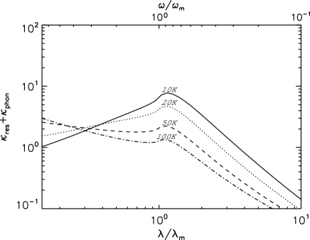
Figure 9: Temperature dependence of the resonant tunneling and phonon induced tunneling relaxation opacity (See Fig. 3 for comparison). The spectra are given in arbitrary units, normalized at $\lambda=100\,{\rm\mu m}$ and $T=10\,K$. Line styles are the same as in Fig. 3.

The hopping relaxation behaves as a distinct spectral feature in the case of narrow barrier height distributions (Sect. 4.4.2, Fig. 6). The amplitude of the effect rises with frequency as $\kappa_{\rm hop}\sim\omega^{2}$, until it reaches a maximum at $\omega=\tau_{0}^{-1}\exp(-V_{0}/k_{\rm\tiny B}T)$. At low temperature the location of the maximum is shifted to MHz frequencies. It reaches the FIR/mm region at $T\simeq 100\,K$, a value which depends upon $V_{0}$. The hopping relaxation in the case of wide barrier height distribution, creates a very wide spectral distribution (Fig. 6). The behavior is then $\kappa_{\rm hop}\sim T\omega^{\beta}$ with a frequency-dependent slope value, usually $\beta<1$ (Eq. 89, Fig. 7).

At a given temperature and wavelength, the relative efficiency of the TLS effects compared to the underlying DCD effect is governed by the density and efficiency of the optically active TLS in the material, and so by the value of the parameter $\overline{P}\mu_{\rm b}$. This value should be related to the fluffiness of the material and to the types and densities of defects in its structure.

Generally, the resonant part of the TLS effects is expected to dominate over the other relaxation processes at temperature below 10K, while the TLS hoping mechanism should fully dominate above 30K.

5.4 Model relevance

Recent astronomical observations of the interstellar dust emission in the FIR/mm wavelength range show some unexpected features which can only be related with difficulty to previous knowledge about dust optical properties in that range (Sect. 3.1. All data have to be explained with a blackbody emission modified by a frequency power law, whose exponent is constant over that FIR/mm range, with a temperature independent asymptotic value equal to two. Indeed, very little is known about the optical properties of the dust amorphous state in that range. Often standard synthetic dust permitivities or opacities are used, which fit perfectly the near and mid-infrared observed features on the basis of a sum of Lorentz-type resonant profiles. But in the absence of reliable data and knowledge, the FIR/mm behavior is often only modeled by the vanishing long-wavelength wings of those infrared resonances. In addition some laboratory data on various silicates reveal additional absorption features, strongly temperature dependent in the FIR/mm range.

It is clear that only specific processes with characteristic frequencies located in the FIR/mm region are needed to explain non purely asymptotic features in this spectral domain. Two phenomena satisfying these requirements are known in solid state physics. First, acoustic oscillations with acoustic wavelengths less than grain size have frequencies in the range $3\cdot 10^{10}-3\cdot 10^{12}$ Hz (Sect. 5.1). These acoustic oscillations are ”optically” active (interact with electromagnetic field) in disordered media (Sect. 4.2). Second, tunneling states in the disordered solids have frequencies $\Delta_{0}/h$ falling in the frequency range $5\cdot 10^{6}-5\cdot 10^{11}$ Hz (Sect. 4.4.2).

These two phenomena are linked to disordered material composing amorphous solids and dirty crystalline compounds. This is also the case of interstellar grains. They dominate the FIR/mm emission of the highly amorphous interstellar dust (Sect. 2.5).

The transverse sound oscillations and tunneling between the potential minima in a disorder lattice includes rotation of groups of atoms, limited and influenced by interactions with their neighboring atoms. In the classification of motion into electronic, vibrational and rotational states used in fundamental quantum mechanics, this model refers to rotational motions, when the former dust emissivity models used only asymptotic behavior of electronic and vibrational processes. In that sense, the model proposed here does not replace the former ones, but complements them by taking into account the physical phenomena efficient in the low frequency range.

Both processes are sensitive to the degree and the type of disorder, rather than to the exact chemical composition of the material. As a consequence, the FIR/mm emission profile is governed by a few key-parameters which characterize the disorder. There is no contradiction between this and laboratory results of FIR/mm dust absorption. It is important to investigate the variations of the model parameters in laboratory measurements of various duly characterized samples. For this purpose, the model gives new avenues for such simulations, and such disorder characterization. It is likely that the FIR/mm properties will be more influenced by the type and degree of disorder than by the chemical composition.

It is important to note that the parameter values adopted in this paper were chosen from purely theoretical grounds or from laboratory results obtained on materials that may not be exactly representative of ISM dust particles. We make no attempt in this paper to model the actual astronomical observations. This will be performed in a companion paper. It is important that only the later parameters be used for astronomical purpose. As the type and degree of disorder in interstellar dust should be representative of the amorphous dust formation itself, we hope that this model will open the way to bring new insights about the interstellar medium dust.

6 Conclusion

The continuum FIR/mm emission is generally attributed to an interstellar dust component of amorphous grains, silicate-based, large enough ($\simeq 15-100\,nm$) to radiate at thermal equilibrium. So far the conception of FIR/mm dust emissivity was built on the semi-classical Lorentz or Drude models. They lead in the long wavelength limit to a dust emissivity obeying to a frequency power law, whose exponent (the spectral index) equals 2 and is usually considered as temperature independent. However a growing volume of FIR/mm observational data induces some doubts about the applicability of such models in that wavelength range.

In this context we present a new model for FIR/mm dust emission, based on physical properties of the disordered matter. We consider the interaction between the electromagnetic field and the acoustic oscillations in a Disordered Charge Distribution and a distribution of low energy Two Level Tunneling states. Both mechanisms apply to the amorphous materials with a large degree of universality, independant of the exact chemical nature of the dust.

The proposed model predicts a disordered induced FIR/mm dust emission which dominates over the weak long wavelength wings of the infrared resonances. This emission is strongly temperature dependent, and leads to a millimeter emission enhancement relative to predications from classical models. The FIR/mm emission spectra can not longer be characterized by a constant spectral index over that range. The detailed shape of the emission spectra is governed by a few key parameters which characterize disorder. The exact values of these parameters for interstellar dust should be determined from observations.

Our model is complementary to the classical models which are reliable in the infrared, and adds emission processes due to disorder induced features.

Appendix A TLS optical density of states

The ODOS spectrum for continuous distribution of DOS is calculated by integration of Eq. (68) over the energy plitting $\Delta_{0}$. We use the following polynomial form of the distribution function $p_{\rm\tiny G}(x)$, with $x=\Delta_{0}/\hbar\omega_{\rm m}$

$$p_{\rm\tiny G}(x)=\left\{\begin{array}[]{ll}\frac{7}{8}(1+3x^{2})(1-x^{2})&\mathrm{for}\ x<1,\\ \hskip 42.67912pt0&\mathrm{for}\ x>1,\end{array}\right.$$ (102)

Equation (102) is a least square polynomial fit to Eq. (70), removing the discontinuity at x=1. A similar result is obtained using the first Fourier harmonics of Eq. (70).

The calculated ODOS spectrum is given by $G(\omega)=\overline{P}\mu_{\rm b}^{2}g(x)$ with $x=\omega/\omega_{\rm m}$ and

$$g(x)=\left\{\begin{array}[]{ll}1+x^{2}g_{1}(x)&\mathrm{for}\ x<1,\\ 1+x^{2}g_{1}(x)-g_{2}(x)\sqrt{1-x^{-2}}&\mathrm{for}\ x>1,\end{array}\right.$$ (103)

with

$$g_{1}(x)=4(5-6x^{2})/15,$$ (104)

$$g_{2}(x)=8(1-x^{2})(2+3x^{2})/15..$$ (105)

In the low frequency approximation ($\omega\ll\omega_{\rm m}$) we have $p_{\rm\tiny G}\approx 1$ and the ODOS function $G(\omega)$ does not depend on $\omega$, in agreement with previous results of the TLS theory.

Appendix B Evaluation of simplified equation for tunneling relaxation calculation.

A use of simplified single integral expression of Bösch (Eq. 83) instead of full double integral equation used here (Eq. 81) is based on assumption that income from asymmetric states is negligible. This approach gives correct result for resonant absorption (Eq. 68) where integrand term $(1-\Delta_{0}/\hbar\omega)^{-1/2}$ amplify weight of symmetric states $\Delta_{0}\approx\hbar\omega$. Another situation takes place for relaxation absorption (Eq. 81) where integrand term $(1-\tau_{1}/\tau)^{+1/2}$ emphasize weight of asymmetric states $\tau\gg\tau_{1}$. Direct calculations give discrepancy of results more than hundred times. A comparison could be made without detailed calculation be consideraton of noncoinsiding terms in integrand expressions in integrals over d$E$. In case of (Eq. 83) it is $f_{1}(\omega,\tau)=\omega^{2}\tau_{1}/(1+\omega^{2}\tau_{1}^{2}).$
In case of (Eq. 81)

$$f_{2}(\omega,\tau)=\int^{\infty}_{\tau_{1}}\sqrt{1-\frac{\tau_{1}}{\tau}}\frac{\omega^{2}\mathrm{d}\tau}{(1+\omega^{2}\tau^{2}}.$$ (106)

It is not difficult to define the asymptotics of both functions

$$f_{1}(\omega,\tau_{1})\approx\left\{\begin{array}[]{ll}\omega^{2}\tau_{1}&\mathrm{for}\ \omega\tau_{1}\ll 1\\ \tau_{1}^{-1}&\mathrm{for}\ \omega\tau_{1}\gg 1\end{array}\right.$$

$$f_{2}(\omega,\tau_{1})\approx\left\{\begin{array}[]{ll}\omega\pi/2&\mathrm{for}\ \omega\tau_{1}\ll 1\\ (2/3)\tau_{1}^{-1}&\mathrm{for}\ \omega\tau_{1}\gg 1\end{array}\right.$$

The asymptotic behaviors of $f_{1}$ and $f_{2}$ are different and the simplified equation is not accurate also for wide region of values of parameters.

Appendix C Calculation of integral for tunneling relaxation spectrum.

The function $F_{\rm phon}(\omega,T)$ (Eq. 4.4.1) can be simplified into a function of a single parameter $F_{\rm phon}(p)$ with $p=a\omega/(2k_{\rm\tiny B}T)^{3}$ through a change of variables to the dimensionless variables $x=\arctan(\omega\tau)$ and $y=\tanh(E/2k_{\rm\tiny B}T)$. Equation 4.4.1 then writes

$$F_{\rm phon}(p)=\int^{1}_{0}\int^{\pi/2}_{x_{1}}\sqrt{1-\frac{\tan x_{1}}{\tan x}}\ \mathrm{d}x\mathrm{d}y,$$ (107)

where

$$x_{1}=\arctan(p\ y\textrm{ arcth}^{-3}y),$$ (108)

The function $F_{\rm phon}(p)$ can be further approximated using a fit of the form,

$$F_{\rm phon}(p)=F_{\rm phon}(p_{i})\left(\frac{p}{p_{i}}\right)^{\beta_{2\,i}},\ p_{i}<p<p_{i+1}.$$ (109)

Precalculated values of the function $F_{\rm phon}$ and the coefficients $\beta_{2}$ entering the interpolated form are given in Tab. 3.

Table 3: Values of $F_{\rm phon}(p_{i})$ and $\beta_{2}(p_{i})$ entering the interpolated form of $F_{\rm phon}(p)$ in Eq. 109.

$p_{i}$	$F_{\rm phon}(p_{i})$	$\beta_{2}(p_{i})$
0.001	1.4696	-0.0321
0.002	1.4313	-0.0446
0.005	1.3604	-0.0678
0.01	1.2875	-0.0924
0.02	1.1948	-0.1248
0.05	1.0393	-0.1826
0.1	0.8984	-0.2397
0.2	0.7433	-0.3090
0.5	0.5334	-0.4185
1	0.3866	-0.5114
2	0.2623	-0.6084
5	0.1417	-0.7343
10	0.0826	-0.8208
20	0.0455	-0.8950
50	0.0194	-0.9659
100	0.0098	-0.9897
200	0.0049	-0.9969
500	0.0020	-1.0000
1000	0.0010	…

Appendix D Calculations of integral for hopping relaxation

Following the TLS formalism, the hopping relaxation spectrum can be computed as the integral of Eq. (77) over a distribution of TLS and barrier heights, taking into account that in contrast to tunneling relaxation, the time constant $\tau$ depends on barrier height $V$ according to Eq.  (87) and does not depend directly on TLS parameters $\Delta_{0}$ and $\Delta$:

$$\chi_{0}^{\prime\prime}(\omega)=\frac{\mu_{\rm b}^{2}}{3k_{\rm\tiny B}T}\int_{0}^{\infty}\int_{-\infty}^{+\infty}\int_{0}^{\infty}\frac{\overline{P}}{\Delta_{0}}P(V)\times$$ (110)

$$\times \frac{\Delta^{2}}{E^{2}}\textrm{sech}^{2}\Big{(}\frac{E}{2k_{\rm\tiny B}T}\Big{)}\frac{\omega\tau}{1+(\omega\tau)^{2}}\ \mathrm{d}\Delta_{0}\ \mathrm{d}\Delta\ \mathrm{d}V.$$

For calculating this expression, the convention of Hunklinger and Schickfus (Hunklinger81 (1981)) is used, which allows to reduce the triple integral to a single integration over distribution $P(V)\mathrm{d}V$, where $P(V)$ is taken to be Gaussian. This convention suggests the independence of the distribution $P(\Delta_{0},\Delta)$ and $P(V)$, which permits to separate the integrals and transforms Eq. (110) into Eq. (87), in a form similar to that of Fitzgerald et al. (2001b ). In this case $P(V)$ is an independent Gauss probability distribution following the standard normalization

$$\int_{0}^{\infty}P(V)\ \mathrm{d}V=1$$

which defines the normalization coefficient $C_{V}$ in Eq. (79) as

$$C_{V}=\frac{1}{V_{0}\sqrt{\pi}}\Big{[}\frac{1}{2}{\rm Erf}\Big{(}\frac{V_{\rm m}-V_{\min}}{V_{0}}\Big{)}+\frac{1}{2}\Big{]}^{-1},$$ (111)

where the term in brackets is usually about unity.

The coefficient $B_{\rm hop}(T)$ in Eq. (87) is equal to

$$B_{\rm hop}(T)=\frac{4\pi}{c\sqrt{\epsilon^{\prime}}}\frac{(\epsilon^{\prime}+2)^{2}}{9}\frac{2}{3}\overline{P}\mu_{\rm b}^{2}$$

$$\times\int_{\Delta_{0}^{\min}}^{\infty}\int_{\Delta_{0}^{\min}}^{E}\textrm{sech}^{2}\Big{(}\frac{E}{2k_{\rm\tiny B}T}\Big{)}\sqrt{1-\frac{\Delta_{0}^{2}}{E^{2}}}\frac{\mathrm{d}\Delta_{0}}{\Delta_{0}}\frac{\mathrm{d}E}{k_{\rm\tiny B}T}=$$

$$=\frac{4\pi}{c\sqrt{\epsilon^{\prime}}}\frac{(\epsilon^{\prime}+2)^{2}}{9}\frac{2}{3}\overline{P}\mu_{\rm b}^{2}(\ln\frac{k_{\rm\tiny B}T}{\Delta_{0}^{\min}}+C_{1}),$$ (112)

where the constant $C_{1}$ is given by

$$C_{1}=\ln 4-1+\int_{0}^{1}\ln{\rm arcth}\ x\ \mathrm{d}x\ =\ -0.441.$$ (113)

The integral (D) over d$\Delta_{0}$ has been determined precisely. Integrating over d$E$ was performed assuming that terms of order $\Delta_{0}^{\min}/k_{\rm\tiny B}T$ and higher orders could be neglected, taking into account that $\Delta_{0}^{\min}/k_{\rm\tiny B}T\ll 1$.

References

- (1) Agladze N.I. et al. 1996, ApJ, 462, 1026
- (2) Agladze N.I., Sievers A.J. 1998, Phys. Rev. Lett., 80, 4209
- (3) Agladze N.I., Sievers A.J., Jones S.A., Burlitch J.M., Beckwith S.V.W. 1994, Nature, 372, 243
- (4) Allamandola L.J., Tielens A., Barker J.R. 1985, ApJ, 290, L25
- (5) Anderson P.W., Halperin B.I., Varma C.M. 1972, Phil. Mag., 25, 1
- (6) Andre P. et al. 1993, ApJ, 406, 122A
- (7) Andriesse C.D. 1974, A&A37, 257
- (8) Barreiro, R. B. et al., 2006, MNRAS, in press
- (9) Bennett, C. L. et al. 2003, ApJS, 148, 97
- (10) Bernard J.-P. et al. 1999, A&A, 347, 640
- (11) Bösch M.A. 1978, Phys. Rev., 40, 879
- (12) Bosomworth D.R., 1967, Phys. Rev., 157, 709
- (13) Boudet N. et al. 2002, in Chemistry as a Diagnostic of Star Formation, ed. C. Curry and M. Fich (NRC Press, Ottawa, Canada), 257
- (14) Boudet N., Mutschke H., Nayral C., J ger C., Bernard J.-P., Henning T., Meny C.,2005, ApJ, 633, 272
- (15) Bouchet, F. R., Gispert, R. 1999, New A, 4, 443
- (16) Brucato J.R., G. Strazzulla et al. 2004, A&A, 413, 395
- (17) Chandler C.J. et al. 1995, ApJ, 455L, 93
- (18) Debye P. 1914, Ann. Physique 43, 49
- (19) Desert F.-X., Boulanger F., Puget J.L. 1990, A&A, 237, 215
- (20) Draine B.T., Anderson N. 1985, ApJ, 292, 494
- (21) Draine B.T., Lee H.M. 1984, ApJ, 285, 89
- (22) Draine B.T., Li A. 2001, ApJ, 551, 807
- (23) Dupac X. et al. 2001, ApJ, 553, 604
- (24) Dupac X. et al. 2002, A&A, 392, 691
- (25) Dupac X., Bernard J.-P. et al. 2003, A&A, 404, L11
- (26) Dupac X., del Burgo C. et al. 2003, MNRAS, 344, 105
- (27) Dwek E. et al. 1997, ApJ, 475, 565
- (28) Ewald P. P., 1922, Naturwiss. 10, 1057
- (29) Finkbeiner D.P., Davis M., Schlegel D.J. 1999, ApJ, 524, 867
- (30) Fitzgerald S.A., Campbell J.A., Sievers A.J., 1994, Phys. Rev. Lett. 73, 3105
- (31) Fitzgerald S.A., Sievers A.J., Campbell J.A. 2001a, J. Phys. Condens. Matter, 13, 2177
- (32) Fitzgerald S.A., Campbell J.A., Sievers A.J. 2001b, J. Phys. Condens. Matter, 13, 2095
- (33) Galliano F., Madden S.C., Jones A.P., Wilson C.D., Bernard J.-P. Le Peintre F., 2003, A&A, 407, 159
- (34) Galliano, F., Madden, S. C., Jones, A. P., Wilson, C. D., & Bernard, J.-P. 2005, A&A, 434, 867
- (35) Gordon M.A. 1988, ApJ, 331, 509
- (36) Gordon M.A. 1990, ApJ, 352, 636
- (37) Gromov V. et al. 2002, in Experimental Cosmology at mm-waves, ed. M. De Petris, M. Gervasi, Amer. Inst. of Phys. Conf. Proc. Ser., 616, 205
- (38) Hadni A., 1970, in S.S. Mitra and S. Nudelman (eds.), Plenum Press, New York, 561
- (39) Henning T., Mutschke H. 1997, A&A, 327, 743
- (40) Heuer A. 1997, Phys. Rev. Lett., 78, 4051
- (41) Hubbard B.E. et al. 2003, Phys. Rev. B, 67, 144201
- (42) Hunklinger S., Schickfus, M. v., 1981, in Amorphous Solids: Low Temperature properties, ed. W.A. Phillips (Springer-Verlag), 81
- (43) Jäckle J. 1972, Z. Physik A, 257, 212
- (44) Jäger, C.D. Fabian et al. 2003, A&A, 401, 57
- (45) Kemper, F., W. J. Vriend, et al. 2004, ApJ, 609, 826
- (46) Koike C., Hasegawa H., Manabe A. 1980. Ap&SS, 67, 495
- (47) Kühn R. 2003, Europhys. Lett., 62, 313
- (48) Lamarre J.-M., 1994, Infrared Phys. and Techn., 35, 277
- (49) Lamarre J.M. et al. 2003, New A Rev., 47, 1017
- (50) Landau L.D., Lifshits E.M. 1982, Course of Theoretical Physics, vol. VIII (Moscow, Nauka)
- (51) Leger A., Puget J.L. 1984, A&A, 137, L5
- (52) Li A., Greenberg J.M. 1997, A&A, 323, 566
- (53) Mathis J.S., Rumpl W., Nordsieck K.H. 1977, ApJ, 217, 425
- (54) Mennella V. et al. 1998, ApJ, 496, 1058
- (55) Mon K.K., Chabal Y.J. and Sievers A.J., 1975, Phys. Rev. Lett., 35, 1352
- (56) Naselsky, P. D. et al., 2005, Int. J. Mod. Phys. D, 14, 1273
- (57) Oldham P. et al. 1994, A&A, 284, 5590
- (58) Pajot F., 2006, A&A, 447, 769
- (59) Phillips, W. 1972, J. Low Temp. Phys., 11, 757
- (60) Phillips W. 1987, Rep. Prog. Phys., 50, 1657
- (61) Rast H.E., Caspers H.H., Miller S.A. 1968, Phys. Rev. 171, 1051
- (62) Reach W.T., Dwek E., Fixsen D.J., Hewagama T. et al., 1995, ApJ, 451, 188
- (63) Ristorcelli I. et al. 1998, ApJ, 496, 267
- (64) Rubens H. and Hertz G., 1912, Berlin. Ber. 14, 256
- (65) Schlömann E. 1964, Phys. Rev. A, 135, 413
- (66) Schwartz P. 1982, ApJ, 252, 589
- (67) Serra G. et al. 2002, Advances in Space Research 30, 1297
- (68) Sievers A.J., Tu J., Agladze N., FitzGerald S.A., Campbell J.A., 1998, Physica B, 244, 159
- (69) Stepnik B. et al. 2003 clim.conf., 187 Cross-Calibration of PRONAOS & ISO, in The Calibration Legacy of the ISO Mission (ESA SP-481)
- (70) Stepnik B. et al. 2003, A&A, 398, 551
- (71) Strom U., Taylor P.C. 1977, Phys. Rev., 16, 5512
- (72) von Schickfus M., Hunklinger S., Pich L. 1975, Phys. Rev. Lett., 35, 876
- (73) von Schickfus M., Hunklinger S. 1976, J. Phys. C, Solid State Phys., 9, L439
- (74) Tamm I. E. 1930, Z. Physik, 60, 345
- (75) Tegmark, M., Eisenstein, D. J., Hu, W., de Oliveira-Costa, A., 2000, ApJ, 530, 133
- (76) Vinogradov, V. S. 1960, Fiz. Tverd. Tela, 2, 2622 (English transl. 1961, Sov. Phys. - Solid St. 2, 2338)
- (77) Walker C. et al. 1990, ApJ, 349, 515
- (78) Weiland J.L. et al. 1986, ApJ, 306, L101
- (79) Woody D. et al. 1989, ApJ, 337, 41
- (80) Wright E. et al. 1992, ApJ, 396, L13