Do long-duration GRBs follow star formation?

We compare the luminosity function and rate inferred from the BATSE long bursts peak flux distribution with those inferred from the Swift peak flux distribution. We find that both the BATSE and the Swift peak fluxes can be fitted by the same luminosity function and the two samples are compatible with a population that follows the star formation rate. The estimated local long GRB rate (without beaming corrections) varies by a factor of five from 0.05 Gpc^-3yr^-1 for a rate function that has a large fraction of high redshift bursts to 0.27 Gpc^-3yr^-1 for a rate function that has many local ones. We then turn to compare the BeppoSax/HETE2 and the Swift observed redshift distributions and compare them with the predictions of the luminosity function found. We find that the discrepancy between the BeppoSax/HETE2 and Swift observed redshift distributions is only partially explained by the different thresholds of the detectors and it may indicate strong selection effects. After trying different forms of the star formation rate (SFR) we find that the observed Swift redshift distribution, with more observed high redshift bursts than expected, is inconsistent with a GRB rate that simply follows current models for the SFR. We show that this can be explained by GRB evolution beyond the SFR (more high redshift bursts). Alternatively this can also arise if the luminosity function evolves and earlier bursts were more luminous or if strong selection effects affect the redshift determination.

1 Introduction

Gamma ray bursts (GRBs) are one of the most powerful events in the universe. The high energy photons emitted travel from cosmological distance tracing the star formation history in the universe. Our understanding of long ($T_{90}>2$sec ) GRBs and their association with stellar collapse follows from the discovery in 1997 of GRB afterglow and the subsequent identification of host galaxies, redshift measurements and detection of associated Supernovae.

However the number of GRBs with a measured redshift is still limited. Only a small fraction of the BeppoSax/HETE2 bursts have measured redshifts. It was expected that Swift would allow further insight into the redshift properties of these objects. Indeed, the ability of Swift to locate and follow-up fainter bursts than the previous satellites, has allowed more distant bursts to be studied. The mean redshift of the BeppoSax/HETE2 sample was $z_{mean}=1.4$, while bursts discovered by Swift now have $z_{mean}=2.8$. The number of Swift bursts with a measured redshift is still small as only $\sim 30$ bursts out of 130 detected bursts have a known redshift. The selection effects that arise in both samples are not clear and hard to quantify (Fiore et al. 2006). Therefore, at present we cannot derive directly the GRB luminosity function and rate evolution that are fundamental to understand the nature of these objects.

We can constrain the luminosity function and rate distribution by fitting the BATSE and Swift peak flux distributions to those expected for a given luminosity function and GRB rate (Piran 1992, Cohen & Piran 1995, Fenimore & Bloom 1995, Loredo & Wasserman 1995, Horack & Hakkila 1997, Loredo & Wasserman 1998, Piran 1999, Schmidt 1999, Schmidt 2001, Sethi & Bhargavi 2001, Guetta et al. 2005, Guetta & Piran 2005, 2006). Since the observed flux distribution is a convolution of these two unknown functions we must assume one and find a best fit for the other. We assume that the rate of long bursts follows the star formation rate (or a modification of the star formation rate, discussed later) and we search for the parameters of the luminosity function. We show, in the first part of the paper that one can obtain a fully consistent fit for both the BATSE and the Swift peak flux samples.

A more complicated issue is to compare the observed redshift distribution of BeppoSax/HETE2 bursts with the observed redshift distribution of Swift bursts and with the predictions of the models for the rate and luminosity function that were inferred from the peak flux distributions. We turn to this problem in the second part of the paper. Clearly the intrinsic GRB distribution is the same and the differences between the observed distributions should arise from the differences in thresholds, in the observed energy band and from selection effects. These factors determine together the samples of bursts with observed redshifts. Among these factors the issue of selection effects is least understood (see however, Hogg and Fruchter, 1999; Bloom et al. 2003 and Fiore et al. 2007). We attempt to correct the BeppoSAX/HETE2 sample for some of the known selection effects. We also consider two limiting cases in which all the bursts with missing redshifts are either at very low or very high redshifts.

Due to the higher detection thresholds the BeppoSax/HETE2 observed distribution is nearer to us than the Swift one. However, the difference in thresholds is not enough to explain the difference between the two observed redshift distributions. With more Swift high redshift bursts than expected we conclude that either GRBs evolve faster than the SFR (more high redshift bursts), or that the assumption that the luminosity function is independent of z is wrong. Daigne et al. (2005) consider these possibilities and, following a different approach, obtain similar results. We also consider models where the GRB rate is a convolution of the SFR and of a sharp jump in the rate to high values at high redshift. These models could be related to the fact that GRBs seem to be more abundant in low metallicity regions (Fynbo et al., 2003; Vreeswijk et al., 2004). Such a jump could arise, for example, from a low metallicity threshold, below which the GRB rate jumps. This possibility has been explored by Natarajan et al. (2005) whose results are similar to the ones obtained in this work. Nuza et al. (2007) developed a Monte Carlo code that simulates a long GRBs distribution for a model where only low-metallicity massive stars are long GRBs progenitors. The results of their calculations are also in agreement with the ones found in our work. Note, however, that a recent analysis of Fynbo et al. (2006) shows that GRBs occur in environments covering a broad range of metallicity at a given redshift. Alternatively it is possible, but less likely, that the observed distribution is completely determined by still unknown selection effects which dominate the BeppoSAX/HETE2 and the Swift redshift determination in unexpected manners.

2 Luminosity function from the BATSE and the Swift samples

Our methodology follows Guetta et al. (2005). For BATSE we consider all the long GRBs detected while the BATSE onboard trigger was set for 5.5 $\sigma$ over background in at least two detectors, in the energy range 50-300 keV. Among those we took the bursts for which $C_{\rm max}/C_{\rm min}\geq 1$ at the 1024 ms timescale, where $C_{\rm max}$ is the count rate in the second brightest illuminated detector and $C_{\rm min}$ is the minimum detectable rate. These constitute a group of 595 bursts. In our previous paper (Guetta et al. 2005) we have shown that the distribution of minimal rates is very narrow and we can take an average rate that corresponds to a threshold $P^{(50-300)keV}_{\rm lim,BATSE}\sim$ 0.25 ph cm^-2 s^-1.

For Swift we consider all long bursts detected until September 2006 ($\sim 130$) bursts in the energy range 15-150 keV. Swift’s complicated triggering algorithm is not based just on the concept of a minimal flux above the background. Still we can have an estimate of the effective Swift threshold by plotting in Fig. 1 the peak flux distribution. This figure compares the peak-flux cumulative distributions of the Swift GRBs with that of BATSE. The comparison is done in the energy band 50-300 keV, which is the band where BATSE detects GRBs. Note that for this comparison we have converted the BAT 15-150 keV peak fluxes to fluxes in the 50-300 keV band using the BAT peak fluxes and spectral parameters. We find an effective threshold of $P^{(50-300)keV}_{\rm lim,Swift}\sim 0.18$ ph cm^-2 s^-1 in agreement with what found by Gorosabel et al. (2004). Note that within the Swift band this threshold corresponds to $P^{(15-150)keV}_{\rm lim,Swift}\sim 0.4$ ph cm^-2 s^-1. The sensitivity of BeppoSax, HETE2 and Swift has been studied in detail by Band (2003, 2006). Band (2006) also studied the sensitivity of BAT instrument as a function of the combined GRB temporal and spectral properties. We refer to these papers for more details on these topics. The values of sensitivities used in this paper are in agreement with Band’s results.

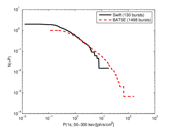
Figure 1: The observed BATSE and Swift peak flux cumulative distributions in the 50-300 keV energy range

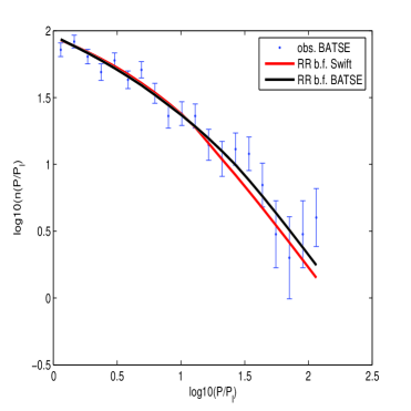
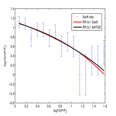
Figure 2: a) left panel: The predicted differential distribution (n(P/P_lim) with the luminosity function parametrs that best fit the BATSE sample (black curve) and the Swift sample (red curve) with a RR-SFR vs. the observed n(C_max/C_min) taken from the BATSE catalog. b) right panel: The predicted differential distribution (n(P/P_lim) with the luminosity function parametrs that best fit the BATSE sample (black curve) and the Swift sample (red curve) with a RR-SFR vs. the observed Swift n(P/P_lim) taken from the Swift catalog

The method used to derive the luminosity function is essentially the one used by Schmidt (1999) and by Guetta et al. (2005). We consider a broken power law with lower and upper limits which are factors of $1/\Delta_{1}$ and $\Delta_{2}$ respectively times the break luminosity $L^{*}$. The luminosity function (of the peak luminosity $L$) in the interval $\log L$ to $\log L+d\log L$ is:

$$\Phi_{o}(L)=c_{o}\left\{\begin{array}[]{ll}(L/L^{*})^{\alpha}&L^{*}/\Delta_{1}<L<L^{*}\\ (L/L^{*})^{\beta}&L^{*}<L<\Delta_{2}L^{*}\end{array}\right.\;,$$ (1)

where $c_{o}$ is a normalization constant so that the integral over the luminosity function equals unity. We stress that the luminosity considered here is the “isotropic” equivalent luminosity, which is the one relevant for detection. It does not include a correction factor due to beaming.

Assuming that long GRBs follow the star formation rate we employ four parametrization of the star formation rate: (i) Model SF2 of Porciani & Madau (2001):

$$R_{GRB}(z)=R_{\rm SF2}(z)=\rho_{0}\frac{23\exp(3.4z)}{\exp(3.4z)+22}$$ (2)

where $\rho_{0}$ is the GRB rate at $z=0$. (ii) The Rowan-Robinson SFR (Rowan-Robinson 1999: RR-SFR) that can be fitted with the expression:

$$R_{GRB}(z)=\rho_{0}\left\{\begin{array}[]{ll}10^{0.75z}&z<1\\ 10^{0.75z_{\rm peak}}&z\geq 1.\end{array}\right.$$

(iii) Model SF3 of Porciani & Madau (2001) with more star formation at early epochs:

$$R_{GRB}(z)=R_{\rm SF3}(z)=\rho_{0}\frac{16\exp(3.4z-0.4)}{\exp(-0.4)(\exp(2.93z)+15)}$$ (3)

(iv) The Star formation history parametric fit to the form of Cole et al. (2001) taken from Hopkins and Beacon (2006). This rate strongly declines with z at high redshift ($z>4$) (v) We consider a toy model where the rate is enhanced at high redshift and the transition is sharp. As mentioned earlier this model might be related, to the lower metallicity at higher redshift. As a toy model we used a SFR as described in model (ii) but at $z>2.5$ is enhanced by a factor of 2:

$$R_{GRB}(z)=\ \left\{\begin{array}[]{ll}R_{\rm RR}(z)&z<2.5\\ 3\,R_{\rm RR}(z)&z\geq 2.5.\end{array}\right.$$

Note that this model resembles but is not the same as the one used by Natarajan et al. (2006) where there is just a jump in the rate and no association with the SFR at all (as not enough details about the model were given in that paper we could not reproduce it here).

(vi) For completeness we consider also a GRB rate that is in between of model (ii) and (v)

$$R_{GRB}(z)=\ \left\{\begin{array}[]{ll}R_{\rm RR}(z)&z<2.5\\ 2\,R_{\rm SF2}(z)&z\geq 2.5.\end{array}\right.$$

We use the standard cosmological parameters $H_{0}=65\leavevmode\nobreak\$ km s^-1 Mpc^-1, $\Omega_{M}=0.3$, and $\Omega_{\Lambda}=0.7$. The different rates are shown in Fig 3.

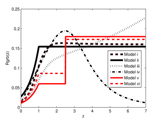
Figure 3: The star formation histories considered in the paper

An important factor is the cosmological k correction. We approximate the typical effective spectral index in the observed range of 50 keV to 300 keV as ($N(E)\propto E^{-1.6}$). This value that was calculated by Schmidt (2001) for BATSE bursts is also adequate for Swift bursts whose average spectral index is $\sim 1.5$. The use of this average correction is justified when we compare estimates of the luminosity based on this average value and on the real spectrum (see Fig. 4 below.)

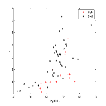
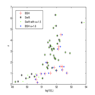
Figure 4: a), left panel: the luminosities and redshifts of the BeppoSAX/HETE2 (BSH in the legend) sample compared with the Swift sample. b), right panel: the same as left panel, also marked are the values of L extrapolated using the average photon index for each sample.

The number of bursts with a peak flux $>P$ is given by:

$$N(>P)=\int\Phi_{o}(L)d\log L\int_{0}^{z_{max}(L,P)}\frac{R_{GRB}(z)}{1+z}\frac{dV(z)}{dz}dz\$$

where the factor $(1+z)^{-1}$ accounts for the cosmological time dilation and $dV(z)/dz$ is the comoving volume element.

We find the best-fitting LF parameters and their dispersion by $\chi^{2}$ minimization. We vary the luminosity function parameters $\alpha$, $\beta$, and $L^{*}$ keeping $\Delta_{1}=100$ and $\Delta_{2}=100$ and inspect the quality of the fit to the observed BATSE peak flux distribution. Once we obtain the best fit parameters for the BATSE sample we test the quality of the fit with both the observed BATSE and the Swift peak flux distributions. We then repeat the same procedure and look for the luminosity function parameters that best fit the Swift sample. Then we check the quality of the fit with these parameters with the observed BATSE and the Swift peak flux distributions. Fig. 2a(2b) depicts a comparison of the observed differential distributions $n(P)\equiv dN/dP$ of BATSE (Swift) with the predicted distribution obtained with the RR-SFR (model (ii)) for the parameters that best fit the BATSE(Swift) data. Also shown on the same figure is the curve obtained using the parameters that best fit the Swift(BATSE) data. Similar curves are obtained for the other models. The $\chi$-square values reported in Table I show the consistency between the Swift and BATSE peak flux samples. The consistency is reassuring. However the fact that we obtain good fits for the data with very different models for the GRB rates reflects the insensitivity, noticed already by Cohen and Piran (1995), of the peak flux distribution to the details of the GRB rate. The peak flux distribution is a convolution of the luminosity function and the GRB rate and different assumptions on the rate simply result in different luminosity function.

The results of the fit are reported in Table 1. These show that the best fit parameters $\alpha$ and $\beta$ are rather robust and they do not depend on the exact shape of the GRB rate chosen and the values of $\alpha$ and $\beta$ found for these rather different models are all within the error bars of each other. To obtain the local rate of GRBs per unit volume, $\rho_{0}$ we need to estimate the effective full-sky coverage of the GRB samples. For BATSE we use 595 (47% of the long GRBs) events detected over 1386 days in the 50-300 keV channel with a sky exposure of 48%. For Swift we consider $\sim 130$ bursts detected in 1.5 yr and a sky coverage is 1/6. The value of $L^{*}$ is around $2.5-5.5\times 10^{51}$erg/sec. It is somewhat higher for models (v) and (vi), as expected because in these cases the intrinsic distribution is farther, and hence stronger pulses are needed. The local rate varies, correspondingly by a factor of 5 from the models (v) and (vi) to model (ii).

The fraction of expected high redshift ($z>6$) Swift bursts vary strongly among the different models: (i) 1.3%, (ii) 0.67% (iii) 3.5%, (iv) 0.07%, (v) 6.2% and (vi) 6.0%. These results are expected in view of the nature of the intrinsic distributions that we consider in these models. The effect of the artificial enhancement of the rate of high redshift bursts in models (v) and (vi) is clearly seen.

It is interesting to compare the fraction of high redshift bursts, that we find, with previous attempts to estimate this number. Using the Amati-like relation $E_{p}\propto L^{0.43}$ Daigne et al. (2005) find 2.5 % for model (i) (SF2-sfr) and 15 % for model (iii) (SF3-sfr) that are somewhat higher than our results. The discrepancy with Daigne et al., (2005) may reflect the inapplicability of the Amati relation (see Nakar and Piran (2005)). The fraction of bursts at $z>4$ of our model (v) is 40%, similar to the result obtained by Natarajan et al. (2005) for their model (iv). Natarajan et al (2005) do not specify the parameters of their model however they also consider an enhancement in the redshift rate at $z\sim 3$ and the fact that we find similar results is reassuring. Bromm and Loeb (2006) consider the contribution of Pop III to high redshift bursts and find that 10% of all Swift bursts can originate at $z>5$. This is equal to what we obtain with our models (v) or (vi). However, it is not clear if this comparison is not a mere coincidence as our models involve a high redshift enhancement in a constant factor above $z>2.5$ and one don’t expect Pop III stars at such “low” redshifts.

The somewhat arbitrary values of $\Delta_{1,2}=(100,100)$ are chosen in such a way that even if there are bursts less luminous than $L^{*}/\Delta_{1}$ or more luminous than $\Delta_{2}L^{*}$ they will constitute only a very small fraction (less than $\sim 1\%$) of the observed bursts. Bursts above $L^{*}\Delta_{2}$ are very bright and are detected to very large distances. However, such strong bursts are very rare. Increasing $\Delta_{2}$ does not add a significant number of bursts (observed or not) and this does not change the results. In particular it does not change the overall rate. $\Delta_{1}$ is more subtle. The luminosity function increases rapidly with decreasing luminosity. Thus, a decrease in $\Delta_{1}$ has a strong effect on the overall rate of GRBs. However, most of the bursts below $L^{*}/\Delta_{1}$ are undetectable by current detectors, unless they are extremely nearby. Even if the luminosity function continues all the way to zero, this will increase enormously the over all rate of the bursts (Guetta & Piran 2006; Guetta & Della Valle 2006) (which will in fact diverge in this extreme example) most of these additional weak bursts will be undetected and the total number of detected bursts won’t increase.

model-sample	Rate(z=0)	$L^{*}$	$\alpha$	$\beta$	$\chi^{2}_{b.f.}$	$\chi^{2}_{\rm other}$
	$Gpc^{-3}yr^{-1}$	$10^{51}$ erg/sec
(i)-BATSE	$0.07^{+0.1}_{-0.05}$	$5.5^{+2.1}_{-3.1}$	$0.3^{+0.3}_{-0.2}$	$2^{+1}_{-0.5}$	$0.82$	1.2
(i)-Swift	$0.10^{0.08}_{-0.06}$	$3.3_{-1.0}^{+3.1}$	$0.1_{-0.05}^{+0.5}$	$2_{-0.4}^{+0.8}$	$0.85$	1.0
(ii)-BATSE	$0.18^{+0.21}_{-0.1}$	$5.5^{+2.1}_{-3.7}$	$0.4^{+0.2}_{-0.3}$	$2.5^{+0.5}_{-1}$	$0.86$	1.1
(ii)-Swift	$0.27^{+0.15}_{-0.22}$	$2.3^{+5.1}_{-0.3}$	$0.1^{+0.5}_{-0.05}$	$2^{+0.4}_{-0.5}$	$0.81$	$0.97$
(iii)-Swift	$0.1^{+0.05}_{-0.03}$	$4^{+2}_{-1}$	$0.1^{+0.3}_{-0.03}$	$2^{+1}_{-0.2}$	$0.82$	$1.1$
(iv)- Swift	$0.11^{+0.08}_{-0.04}$	$3.0^{+1.9}_{-2.8}$	$0.2^{+0.3}_{-0.1}$	$2^{+0.7}_{-0.5}$	0.83	1.2
(v)- Swift	$0.05^{+0.03}_{-0.03}$	$6.5^{+0.8}_{-2}$	$0.2_{-0.1}^{+0.3}$	$1.7^{+0.5}_{-0.3}$	0.85	1.2
(vi)- Swift	$0.07^{+0.03}_{-0.04}$	$7^{+0.8}_{-2}$	$0.2_{-0.1}^{+0.3}$	$2^{+0.2}_{-0.3}$	0.9	1.2

Table 1: Best fit parameters $Rate(z=0)$ , $L^{*}$, $\alpha$ and $\beta$ and their 1-$\sigma$ confidence levels. For each fit we report the $\chi^{2}$ values corresponding to the best fit ($\chi^{2}_{\rm b.f.}$). Also shown are the $\chi^{2}$ values for the fit to the BATSE(Swift) data obtained using the parameters that best fit the Swift(BATSE) sample ($\chi^{2}_{\rm other}$).

3 The redshift distributions

We turn now to the observed redshift distributions of BeppoSAX/HETE2 and Swift. For BeppoSax/HETE2 we consider the observed distribution of all the with an available redshift: 32 bursts from http://www.mpe.mpg.de/ jcg/grbgen.html (excluding GRB980425 with $z=0.0085$). For Swift we consider all bursts with an available redshift: 39 bursts from the Swift home page.

The redshift sample is influenced by selection effects that are hard to quantify. To rectify this problem we compare our models both with the raw data and with corrected samples that attempt take these effects into account. The selection effects are most severe if the redshift determination depends on the identification of emission lines in the spectrum of the host galaxy. Since there are very few emission lines in the range $1.3<z<2.5$ (Hogg & Fruchter, 1999) such redshifts may be missed. For BeppoSAX/HETE2 this is the main mode of redshift determination. We follow, therfore, Hogg & Fruchter (1999) and consider a modified distribution in which all BeppoSAX/HETE2 GRBs with an optical afterglow but without a redshift determination are assigned uniformly in this redshift range $1.3<z<2.5$. Using the data in http://www.mpe.mpg.de/ jcg/grbgen.html we have a total sample of 46 BeppoSAX/HETE2 GRBs: 32 with measured redshift and 14 with no measured redshifts which we assign to this range in a uniform way. For completeness we also check what happens if all bursts with no redshift but with optical afterglow are nearby, that is they are distributed uniformly between $(0<z<1.5)$, or distant, i.e. distributed uniformly between $z=2.3$ and the maximal BeppoSAX/HETE2 redshift $z=4.3$.

The situation concerning Swift bursts is more complicated as most Swift redshifts are obtained using absorption lines in the optical afterglow. The main selection effect in this case is the weakness of the afterglow signal or the optical depth within the host (Fiore et al. 2007). Both selection effects work against high redshift bursts. Lacking a clear model we consider for Swift just the observed data set.

Figure 4 depicts the isotropic peak luminosities and redshifts of the BeppoSAX/HETE2 and Swift samples. This figure shows clearly the differences in thresholds. In the second figure we also plot the values of L for the average photon index assumed in the calculations. As we can see from this figure the values of the peak luminosities obtained using the average spectrum are rather similar to the ones obtained using the real spectrum. Therefore, it is reasonable to use the average spectrum for the k-correction as we have done in this analysis. Another feature seen in this figure is that the Swift redshift distribution shows (seen even more clearly in Fig. 5) a paucity of bursts in the range $1<z<2$. It is not clear if this is statistically significant, but it is apparent in the data. There is no clear selection effect that could give rise to this feature.

Using the different models for the GRB rate and the luminosity function we derive now the expected distribution of the observed bursts’ redshifts:

$$n(z,L)dzd\log(L)=\frac{R_{GRB}(z)}{1+z}\frac{dV(z)}{dz}\Phi_{o}(L)d\log L\ \ .$$ (4)

The expected redshift distribution is:

$$N(z)=\frac{R_{GRB}(z)}{1+z}\frac{dV(z)}{dz}\int_{L_{\rm min}(P_{\rm lim},z)}^{L_{\rm max}}\Phi_{o}(L)d\log L\ ,$$ (5)

where $L_{\rm min}(P_{\rm lim})$ is the luminosity corresponding to minimum peak flux $P_{\rm lim}$ for a burst at redshift z and $L_{\rm max}=L^{*}\times\Delta_{2}=10\,L^{*}$. This minimal peak flux corresponds to the detector’s threshold. For BeppoSax/HETE2 we use, $P^{(50-300)keV}_{\rm lim}\sim 0.5$ ph cm${}^{-2}s^{-1}$, which is roughly the limiting flux for the GRBM on BeppoSAX (Guidorzi 2002). The triggering algorithm for Swift is rather complicated but as shown in Fig. 1 it can be approximated by a minimal rate: $P^{(50-300)keV}_{\rm limSwift}\sim 0.18$ ph/cm²/sec.

Our results are summarized in Table 2 and in Figs. 5 and 6 which present a comparison of the observed (corrected and uncorrected) BeppoSAX/Hete2 and Swift redshift distributions with theoretical models that were obtained from best fits of the model’s parameters to the Swift peak flux distribution. Qualitatively similar results are obtained from best fits to the BATSE peak flux distribution. Fig. 5 depicts the differential distribution of the observed redshifts while Fig. 6 depicts the integrated distribution. The values of the KS test for the different models are shown in Table 2.

The most remarkable feature is that none of the pure SFR models (i-iv) is consistent with the Swift data. This result is consistent with the findings of Daigne et al. (2006). The Swift redshift distribution is inconsistent even with model (iii), that is model SF3 of Porciani and Madau (2001) which is rising at large redshifts. It is consistent only with distributions (v) and (vi) that involve an “artificial” large redshift enhancement compared to the standard SFR model.

Consequently, it is difficult to find models that fit both the Swift and the BeppoSAX/HETE2 data. Models (i), (iii) and (iv) that favor a nearer GRB distribution, are consistent with the BeppoSAX/Hete2 distribution while model (v) that favors a more distant distribution is consistent with the observed Swift redshift distribution. The only combined fit to both data sets is obtained for model (vi) which is consistent with the Swift distribution (KS values $\sim$ 0.19) and with the corrected the BeppoSAX/HETE2 data (KS values $\sim$ 0.17). Model (vi) represents a variation of the rather arbitrary parameters of model (v). Clearly, we can consider a series of models based on RR SFR ranging from no enhancement at high z (model ii) which fits the uncorrected BeppoSAX/HETE2 sample to a very strong enhancement at high z (model v) that fits just the Swift data. In model (vi) we consider an intermediate enhancement which is formally consistent with both the Swift and the modified BeppoSAX/HETE2 data. However, as we discuss later, even in these models and even in the models like, (i), (ii), (iv) that are compatible with BeppoSAX/HETE2 redshift distribution, the two dimensional redshift luminosity distribution shows too many high luminosity bursts. Note that similar results were obtained when we modified SF2 by adding an ad hoc enhancement at large redshift.

Fig.7 depicts a comparison of the theoretical models with two extreme modifications of the BeppoSAX/HETE2 distributions. These modifications attempt to estimate different extreme effects of the selection effects for BeppoSAX/HETE2. In one case we put all bursts with an optical afterglow and an unknown redshift at a large redshift (a uniform distribution in the range in the $2.3<z<4.3$). In the other case we put all these bursts uniformly in z at small redshift ($z<1.3$). The KS values of the comparison with different models are shown in Table 3. We see that putting all the bursts uniformly distributed in the range $0<z<1.3$ has a little effect. Models (like (ii) and (iv)) that are consistent with the uncorrected distribution are consistent with the corrected one and others are now. Putting all bursts with an unknown redshift at $2.3<z<4.3$ has a strong effect. With this correction no SFR can fit the BeppoSAX/HETE2 corrected data and we need a model like (v) or (vi) with a high redshift enhancement. This extreme (high redshift) correction makes the BeppoSAX/HETE2 data compatible with the Swift data. Note, however, that there is no clear reason to choose such a correction.

model	BeppoSAX/HETE2	BeppoSAX/HETE2	Swift
		$1.3<z<2.5$ correction
(i)	$0.04$	$0.69$	$<0.01$
(ii)	$0.63$	$0.03$	$<0.01$
(iii)	$0.01$	$0.27$	$0.03$
(iv)	$0.25$	$0.41$	$<0.01$
(v)	$<0.01$	$0.05$	$0.85$
(vi)	$0.03$	$0.17$	$0.19$

Table 2: KS probability values for the BeppoSax/HETE2 and the Swift samples for theoretical models with parameters that best fit the Swift peak flux distribution

model	BeppoSAX/HETE2	BeppoSAX/HETE2
	$0<z<1.3$ correction	$2.3<z<4.3$ correction
(i)	$0.01$	$0.02$
(ii)	$0.50$	$<0.01$
(iii)	$<0.01$	$0.14$
(iv)	$0.10$	$<0.01$
(v)	$<0.01$	$0.56$
(vi)	$<0.01$	$0.18$

Table 3: KS probability values for two extreme corrections to the BeppoSax/HETE2 sample. The low redshift correction adds all the bursts with optical afterglow and unknown redshift uniformly in the region $0<z<1.3$ and the high redshift correction adds them uniformly at the region $2.3<z<4.3$. The theoretical models use parameters that best fit the Swift peak flux distribution

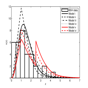
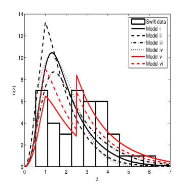
Figure 5: The predicted and the observed differential distributions of the GRBs redshift for the different models (a) left panel - Swift data with theoretical models with $P_{lim}=0.18$ (b) right panel BeppoSax/HETE2 (BSH in the legend) and the models with $P_{lim}=0.5$.

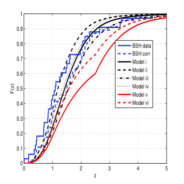
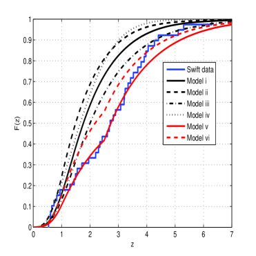
Figure 6: The predicted and the observed cumulative distributions of the GRBs redshift for the different models (a) left panel - Swift data with theoretical models with $P_{lim}=0.18$ (b) right panel BeppoSAX/HETE2 and the models with $P_{lim}=0.5$. For BeppoSAX/HETE2 we also show the distribution where selection effects are taken into account assuming that all the GRB with no redshift but with optical afterglow lie in the range $1.3<z<2.5$.

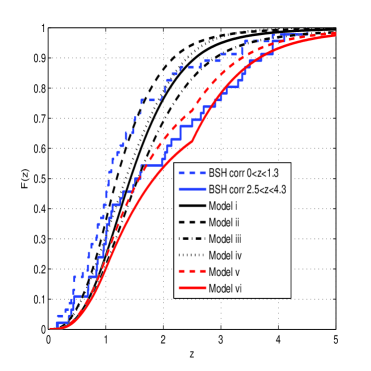
Figure 7: The predicted and the observed cumulative distributions of the GRBs redshift for BeppoSAX/HETE2 sample and the models with $P_{lim}=0.5$. We also show the distribution where selection effects are taken into account assuming that all the GRB with no redshift but with optical afterglow lie in the range $0<z<1.3$ and $2.3<z<4.3$.

Fig. 8 depicts a comparison of the two dimensional redshift and luminosity distributions between the BeppoSAX/HETE2 data and model (ii). Naturally, we include here only bursts with known redshifts. Several features are apparent. First, the estimate of $P_{lim}=0.5$ for BeppoSAX/HETE2 is reasonable. Only one burst is detected in the “forbidden” region with a lower peak flux. However, it is clear that there is no good fit between the model and the observed distribution. The lack of bursts in the range $1.5<z<3$ may be explained by selection effects. However, in addition, there are significantly more high luminosity bursts than predicted by the model. It is clear that even though the KS test of the integrated redshift distribution for this model suggests that the model is consistent with the observed distribution the two dimensional distribution of luminosities and redshifts is inconsistent. Similar, or worse results are obtained for this data with all other models that we have considered including, in particular, model (vi).

A similar comparison between model (v) and the Swift data is shown in Fig 9. Here there are several bursts in the forbidden region in the upper left part of the plot where the peak flux is below $0.18$ph/cm²/s. These bursts reflect the fact that Swift’s trigger is not based just on peak flux counts. However as these bursts cluster very close to the line $P_{lim}=0.18$ph/cm²/s we find that the complicated triggering algorithm of Swift is not an issue. The fit of the observed data to the model is clearly better than the one seen in Fig. 8. Still it is not compelling. Here the basic problem can be seen also in Fig. 5 that depicts the observed differential redshift distribution of Swift bursts. The paucity of bursts in the range $1<z<2$ hints towards a two population model - or towards a high redshift enhancement of the sort that we have crudely modeled in (v). Unlike the BeppoSAX/HETE2 sample we don’t see here a significant fraction of high luminousity bursts (as compared with the model) but again there are hints towards a broader luminosity function that the one we use.

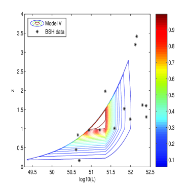
Figure 8: The two dimensional probability distribution of expected redshift and luminosity for the luminosity function parameters that best fit the Swift peak flux distribution considering a RR-sfr and $P_{lim}=0.5$ph/cm²/s. Contour lines are 0.9,0.8… 0.01 of the maximum. Also marked are the BeppoSax/HETE2 (BSH in the legend) GRBs with a known redshift and spectral index. Note that there is only one burst in the ”forbidden” region in the upper left part of the plot where the peak flux is below $0.5$ph/cm²/s.

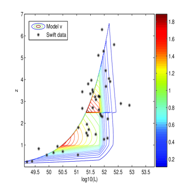
Figure 9: The two dimensional probability distribution of expected redshift and luminosity for the luminosity function parameters that best fit the Swift peak flux distribution considering model (v) and $P_{lim}=0.18$ph/cm²/s. Contour lines are 0.9,0.8… 0.01 of the maximum. Also marked are the Swift GRBs with a known redshift. Note that there are several bursts in the ”forbidden” region in the upper left part of the plot where the peak flux is below $0.18$ph/cm²/s. These bursts reflect the fact that Swift’s trigger is not based just on peak flux counts. However as these bursts cluster very close to the line $P_{lim}=0.18$ph/cm²/s we find that the complicated triggering algorithm of Swift if not an issue here.

4 Conclusions and Implications

We find that Swift GRBs do not follow the SFR as described by several different models (i-iv). Given these SFRs there is no luminosity function that can fit both the Swift observed peak flux and the z-distributions. We were able to obtain a reasonable fit when we considered a GRB rate function that included a high redshift enhancement. This might be related to suggestions that long GRBs arise preferably in low metallicity regions (Fynbo et al 2003; Vreeswijk et al., 2004). But it could arise from other reasons. We used a simple toy scheme to model this enhancement. Because of the very crude nature of the model and the limited scope of the available data we did not try to optimize extensively the parameters of this model. It was reassuring that we obtained a reasonable fit with such a simple model and without an extensive search for the parameters. It is remarkable that the enhancement arises in the high redshift range, where the bursts and their afterglow are weaker and hence selection effects are expected to reduce rather than increase the number of bursts with detected redshifts.

We mention now the strange paucity of Swift bursts with $1<z<2$. If real and not just a statistical fluctuation or a result of an unknown selection effect this paucity may indicate: (a) A jump in long GRB rate or another factor at higher redshifts; (b) A dependence of the luminosity function on the rate or even the existence; (c) The appearance of two populations one at lower redshift and another one at higher redshifts (which can be viewed as a special case of a z dependence of the luminosity function). While these speculations are intriguing it is clear that it is essential to determine the selection effects that control the samples of GRBs with determined redshifts before far reaching conclusions are made.

The only GRB rate and luminosity functions that are consistent with these distributions and with both observed redshift distributions (of BeppoSAX/HETE2 and of Swift) is a one with an enhanced GRB rate at large redshift. This consistency is achieved only after we modified the BeppoSAX/HETE2 sample by adding all bursts with no redshift in the range $1.5<z<2.5$ in which there are no strong emission lines and redshift identification is difficult (Hogg & Fruchter, 1999) or if we put all those bursts, artificially, at high redshifts $2.3<z<4.5$. However, as the two dimensional distribution of redshifts and luminosities of the Bepposax/HETE2 does not seem to fit the model we do not assign a great significance to this fact.

Another important result is that the BATSE and Swift peak flux distributions are consistent with each other and with the estimated limiting fluxes for detection for the two detectors. The combined analysis suggests that the local rate of GRBs (without a beaming correction) can be determined up to a factor of approximately five and it ranges between 0.05Gpc^-3yr^-1 for a rate function that has a large fraction of high redshift bursts to 0.27Gpc^-3yr^-1. Note that the inferred low local rates, $\sim 0.05$ Gpc^-3yr^-1, which are about an order of magnitude lower than previous estimates (Guetta, Piran & Waxman, 2005), arise from the models that involve metallicity enhancement at large redshifts. These rates do not include the beaming correction which is of order $\sim 100$. Even with this correction these rates correspond to a local rate of a burst per $2\times 10^{6}$ years per galaxy, indicating that strong GRBs are a very rate phenomenon. However, the actual rate of weak bursts could be much higher if indeed there is a large population of very low luminosity bursts, as inferred from the detection of GRB 060218 (Soderberg et al., 2006). These models predict, on the other hand, a relatively large fraction of about 6% of high redshift $(z>6)$ Swift bursts.

When considering the BeppoSAX/HETE2 redshift distribution on its own it seemed that even luminosity functions and rates that fit the peak flux distribution and the observed redshift distributions do not fit the two dimensional luminosity and redshift distribution. The paucity of bursts with redshifts between $1.5<z<2.5$ can be explained by the selection effect mentioned earlier. However, the excess of very luminous low redshift bursts is unexpected and indicates that other selection effects that favor identification redshift determination of such bursts take place and possibly dominate the BeppoSAX/HETE2 sample. If correct this has potential implications to other statistical information that has been determined from this data sample.

References

- (1) Band, D., 2003, ApJ 588, 945.
- (2) Band, D., 2006, ApJ 644, 378.
- (3) Bloom J., 2003, ApJ 125, 2865.
- (4) Cohen E., Piran T., 1995, ApJ, 444, L25
- (5) Cole, S. et al, 2001, MNRAS 326, 255.
- (6) Daigne, F., Rossi, E. M. & Mochovitch, R., 2006, MNRAS 373, 1034.
- (7) Fenimore, E. & Bloom, J., 1995, ApJ 453, 25
- (8) Fiore, F., Guetta, D., Piranomonte, S., D’Elia, V. & Antonelli, A. astro-ph/0704.2189 A& A in press.
- (9) Fynbo, J. et al., 2006, A&A 451, L47.
- (10) Fynbo, J. et al., 2003, A&A 406, L63.
- (11) Guetta, D., Piran, T. & Waxman E., 2005, ApJ, 619, 412. (GPW).
- Guetta & Piran (2005) Guetta, D., & Piran, T. 2005, A&A, 435, 421.
- Guetta & Piran (2005) Guetta, D., & Piran, T. 2006, A&A, 453, 823.
- (14) Guetta, D. & Della Valle, M., 2006, ApJ 657, L73.
- (15) Guidorzi, C. 2002, Ph. D. Thesis University of Ferrara.
- (16) Hogg, D. & Fruchter, A., 1999, ApJ 520, 54.
- (17) Hopkins, A. M. & Beacom, J. F., 2006, ApJ 651, 142.
- (18) Horack, J. M . & Hakkila, J., 1997, ApJ 479, 371.
- (19) Loredo, T. & Wasserman, Ira M., 1998, ApJ 502, 75L
- (20) Natarajan, P. et al., 2005, MNRAS 364, L8.
- (21) Nuza, S. E., 2007, MNRAS 375, 665.
- (22) Pettini, M. et al., 2003, ApJ 594, 695.
- (23) Piran, T., 1992, ApJ 389, L45.
- (24) Porciani, C., and Madau, P., 2001, ApJ 548, 522.
- Price et al. (2005) Price, P. A. et al. 2005, GRB Circular Network, 3612, 1.
- (26) Rowan-Robinson, M., 1999, Ap&SS266, 291R.
- (27) Schmidt, M., 1999, ApJ 523, L117.
- (28) Schmidt, M., 2001, ApJ 559, L79.
- (29) Sethi, S. & Bhargavi, S. G., 2001, A&A 376, 10S.
- (30) Soderberg, A., et al., 2006, Nature, 442, 1014.
- (31) Volker, B. & Loeb, A., 2006, ApJ 642, 382.
- (32) Vreeswijk, P. M., Moller, P. & Fynbo, J.P.U., 2003, A&A 409, L5.