Photometric Stellar Variability in the Galactic Center

Abstract

We report the results of a diffraction-limited, photometric variability study of the central 5^′′ $\times$ 5^′′ of the Galaxy conducted over the past 10 years using speckle imaging techniques on the W. M. Keck I 10 m telescope. Within our limiting magnitude of $m_{K}<16$ mag for images made from a single night of data, we find a minimum of 15 K[2.2 $\micron$]-band variable stars out of 131 monitored stars. While large populations of binaries have been posited to exist in this region, both to explain the presence of young stars in the vicinity of a black hole and because of the high stellar densities, only two binaries are identified in this study. First is the previously identified Ofpe/WN9 equal mass eclipsing binary star IRS 16SW, for which we measure an orbital period of $19.448\pm 0.002$ days. In contrast to recent results, our data on IRS 16SW show an asymmetric phased light curve with a much steeper fall-time than rise-time, which may be due to tidal deformations caused by the proximity of the stars in their orbits. Second is the WC 9 Wolf-Rayet star IRS 29N; its observed photometric variation over a few year time-scale is likely due to episodic dust production in a binary system containing two windy stars. Our sample also includes 4 candidate Luminous Blue Variable (LBV) stars (IRS 16NE, 16C, 16NW, 16SW). While 2 of them show variability, none show the characteristic of LBVs large increase or decrease in luminosity. However, our time baseline is too short to rule them out as LBVs. Nonetheless, the lack of evidence for these stars to be LBVs and their coexistence with a significant surrounding population of well established Wolf-Rayet stars is consistent with needing only a single recent starburst event at the Galactic center to account for all of the known, young, massive stars. Among the remaining variable stars, the majority are early-type stars and three are possibly variable due to line of sight extinction variations. For the 7 OB stars at the center of our field of view that have well-determined 3-dimensional orbits, we see no evidence of flares or dimming of their light, which limits the possibility of a cold, geometrically-thin inactive accretion disk around the supermassive black hole, Sgr A^∗.

1. Introduction

The stellar cluster at the Galactic center (GC) presents a unique opportunity to study the evolution and properties of stars within the sphere of influence of a $3-4\times 10^{6}M_{\odot}$ supermassive black hole (SMBH) (Ghez et al., 2003, 2005; Schödel et al., 2003). Photometric variability offers a useful approach to a number of outstanding questions regarding this stellar population which is composed of a mixture of old giants and young, massive stars. (Krabbe et al., 1991, 1995; Blum et al., 1996a, b, 2003; Figer et al., 2003; Paumard et al., 2001, 2004b, 2006). For example, light curves can easily reveal close binary stars, which are relevant in several ways to our understanding of stars at the Galactic center.

First, binaries on radial orbits that are disrupted by the central black hole may provide a mechanism for capturing young stars from large galacto-centric radii, where the conditions are conducive to star formation, and retaining them at the smaller less hospitable radii where many young stars are found today (Gould & Quillen, 2003). Second, binary companions may facilitate the production of dust around the WC sub-class of Wolf-Rayet stars, which are massive post-main sequence stars undergoing rapid mass loss. While conditions in the hostile environment (high temperatures in particular) of the stellar winds do not favor the formation of dust (Williams et al., 1987), compression within wind-colliding binary systems could overcome this challenge (White & Becker, 1995; Veen et al., 1998; Williams & van der Hucht, 2000; Lefèvre et al., 2005). Third, binaries provide a direct measurement of stellar masses. This is especially helpful for the most massive stars in the Galactic center as it would assist our understanding of the recent star formation history.

Another way in which a photometric variability study constrains the recent star formation history, as well as our understanding of massive star evolution, is the possibility of identifying luminous blue variables (LBVs). There are currently only 12 confirmed Galactic LBVs and 23 additional candidates, with 6 candidates in the Galactic center IRS 16 cluster of stars alone (Clark et al., 2005). The LBV phase plays an important, although poorly constrained, role in stellar evolution, because, during this phase, stars experience significant mass loss, with rates of $\sim 10^{-2}M_{\odot}$/yr during eruptions and as high as high as $10^{-4.5}M_{\odot}$/yr during quiescent phases (Abbott & Conti, 1987; Humphreys & Davidson, 1994; Massey, 2003). From a star formation history stand point, the LBV phase is notable because it is the first of several post main sequence phases that only the most massive stars ($M\gtrsim 60-85M_{\odot}$) may go through before becoming supernovae. Stars stay in this phase for only $\sim 10^{4}$ years (Stothers & Chin, 1996) before entering the Wolf-Rayet phase, which typically lasts a few $\times 10^{6}$ years (Meynet & Maeder, 2005). Less massive stars ($M\gtrsim 40M_{\odot}$) will skip the LBV phase and become Wolf-Rayet stars, but on time-scales longer than that of the more massive stars that experienced an LBV phase. Therefore, in principle, the numbers of LBVs and WR stars can constrain recent star formation histories (e.g. Paumard et al. 2006; Figer 2004). In this context the candidate LBVs at the Galactic center are perplexing in the context of the $\gtrsim 25$ Wolf-Rayet stars located in their immediate vicinity, since in a single starburst event one would not expect to see any WR stars if the most massive stars are just now evolving through the LBV phase. This is similar to the problem posed by the presence of two LBVs in the Quintuplet cluster Figer (2004). If confirmed, the LBV candidates would suggest that this region has undergone multiple recent star forming events or that our understanding of LBV evolution is incomplete.

The photometry of stars in close proximity to the SMBH can also be used to constrain the properties of a possible cold, geometrically-thin inactive accretion disk around Sgr A^∗ which could explain the present-day low luminosity of Sgr A^∗ (Nayakshin & Sunyaev, 2003; Cuadra et al., 2003). In the presence of such a disk, we would expect to see nearby stars eclipsed or reddened when they pass behind the disk.

Very few photometric variable studies of the Galactic center exist. Tamura et al. (1999) introduced the idea that stars close to the Galactic center are expected to have a higher fraction of ellipsoidal and eclipsing variable binaries than the stars in the solar neighborhood, but found very few variable stars and no binary stars. Seeing-limited studies (Tamura et al., 1999; Blum et al., 1996a) are limited to the brightest stars, due to stellar confusion caused by the high stellar densities and proper motions close to the central black hole. With high angular resolution data, Ott et al. (1999) have identified the only known eclipsing binary system in this region (see also DePoy et al. 2004; Martins et al. 2006). Furthermore, they suggest that as much as half of their sample (K $\lesssim$13) may be variable. However, the variability fraction decreases at smaller galactocentric radii starting from $\sim 5\tt^{\prime\prime}$, suggesting that even at a high resolution of 0$\farcs$13 their sensitivity to variability is limited by stellar confusion.

In this paper, we present the results of a stellar variability study of the central 5^′′$\times$5^′′ of our Galaxy, based on ten years of K[2.2 $\mu$m] diffraction-limited images from the W. M. Keck I Telescope ($\theta=0\farcs 05$). The observations are described in §2, and the data and methodology to determine variability in §3. We discuss the variable star population in §4, which includes identification of asymmetries in the light curve of the eclipsing binary star IRS 16SW and the discovery of a likely wind colliding binary star in IRS 29N, and summarize our major findings in §5.

2. Observations

K-band ($\lambda_{o}$ = 2.2µm, $\Delta\lambda$=0.4µm) speckle imaging observations of the Galaxy’s central stellar cluster were obtained with the W. M. Keck I 10 m telescope using the facility near-infrared camera, NIRC (Matthews & Soifer, 1994). Observations taken from 1995 to 2004 have been described in detail elsewhere (Ghez et al., 1998, 2000, 2005; Lu et al., 2005) and new observations on 2005 April 24-25 were conducted in a similar manner, resulting in diffraction-limited images. Each night several thousand short-exposure frames were taken in sets of $\sim 200$, with NIRC in its fine plate scale mode, which has a scale of 20.40 $\pm$ 0.04 mas pixel^-1 and a corresponding field of view (FOV) of 5$\farcs$22 $\times$ 5$\farcs$22 (Matthews et al., 1996). Table 1 lists the date and number of frames obtained for each of the 50 nights of observations used in this study.

3. Data Analysis and Results

3.1. Image Processing

The individual frames are processed in two steps to create a final average image for each night of observation. First, the standard image reduction steps of sky subtraction, flat-fielding, bad pixel correction, optical distortion correction, and pixel magnification by a factor of two are carried out on each frame. Second, the frames from each night of observation are combined using the method of ”Shift-and-Add” (Christou, 1991) with the frame selection and weighting scheme prescribed by Hornstein (2006). In short, each frame is analyzed for Strehl quality using the peak pixel value of IRS 16C, and low quality frames, which do not improve the cumulative signal to noise ratio (SNR) for the observations from each night, are rejected. This typically leaves $\sim$1600 frames for each night or 37% of the original data set (see column 3 of Table 1). The remaining frames for a given night are combined with Shift-and-Add in an average that is weighted by each frame’s peak pixel value for IRS 16C. The final images have typical Strehl ratios of $\sim$0.07 (see column 8 of Table 1). The dataset from each night is also divided into three equivalent quality (and randomized in time) subsets to make three independent weighted Shift-and-Add image subsets, which are used to determine measurement uncertainties and to reject spurious sources.

Table 1List of Observations

Date	Frames	Frames	Num. Stars	Num. Stars	SNR	Strehl
	(Obs.)	(Used)	(Initial)	(Final)
1995 Jun 10	1200	425	54	66	10.3	0.08
1995 Jun 11	2700	1604	95	110	15.0	0.06
1995 Jun 12	2100	1082	107	108	12.0	0.04
1996 Jun 26	4200	585	116	119	19.8	0.04
1996 Jun 27	2300	1260	117	121	20.5	0.04
1997 May 14	3600	1851	63	82	16.7	0.06
1998 Apr 02	2660	1649	119	121	16.3	0.05
1998 May 14	4560	1748	96	114	16.7	0.04
1998 May 15	7030	1953	41	55	9.9	0.06
1998 Jul 04	2280	943	108	114	17.8	0.08
1998 Aug 04	6270	1469	87	107	15.5	0.05
1998 Aug 05	5700	1592	94	103	17.3	0.07
1998 Oct 09	2660	1188	83	99	17.1	0.08
1998 Oct 11	570	450	79	96	15.0	0.05
1999 May 02	7030	1589	115	116	19.9	0.09
1999 May 03	2090	1264	103	114	16.0	0.07
1999 Jul 24	5510	2239	113	119	18.5	0.11
1999 Jul 25	950	788	102	114	15.0	0.06
2000 Apr 21	3040	947	90	112	18.5	0.04
2000 May 19	9880	1970	64	91	10.2	0.09
2000 May 20	7600	2146	81	97	16.5	0.10
2000 Jul 19	8740	1939	111	116	17.1	0.07
2000 Jul 20	3420	1454	111	119	19.8	0.09
2000 Oct 18	2280	1807	82	107	15.1	0.05
2001 May 08	1520	889	111	124	20.1	0.04
2001 May 09	6270	1990	76	100	13.1	0.08
2001 Jul 28	4180	1752	99	104	20.0	0.13
2001 Jul 29	6080	1751	105	115	19.0	0.07
2002 Apr 23	7410	1669	117	119	17.2	0.05
2002 Apr 24	7790	1882	104	113	19.6	0.06
2002 May 23	1900	1249	66	84	18.3	0.07
2002 May 24	2660	1537	85	100	17.7	0.09
2002 May 28	2850	1866	59	80	13.2	0.06
2002 May 29	3420	1552	86	104	16.8	0.07
2002 Jun 01	5510	1992	43	53	7.7	0.09
2002 Jul 19	4370	1115	41	57	7.0	0.07
2002 Jul 20	3990	1355	51	64	11.0	0.06
2003 Apr 21	5130	1799	93	107	19.1	0.04
2003 Apr 23	5320	1970	69	87	13.2	0.05
2003 Jul 22	5130	1718	70	94	16.6	0.08
2003 Sep 07	4560	1795	108	112	16.3	0.07
2003 Sep 08	4370	1223	97	110	12.3	0.07
2004 Apr 29	6840	1181	53	68	14.5	0.11
2004 Apr 30	4180	1203	98	105	16.6	0.05
2004 Jul 25	5320	2007	98	110	18.1	0.08
2004 Jul 26	8550	2309	33	38	6.7	0.08
2004 Aug 29	3230	1328	120	122	21.0	0.10
2005 Apr 24	7410	2195	51	60	11.6	0.07
2005 Apr 25	9500	2035	116	116	20.8	0.05
2005 Jul 26	6650	1497	98	113	19.0	0.06

Note. — All observations are speckle K-band ($\lambda_{o}$ = 2.2µm, $\Delta\lambda$=0.4µm) images.

Sources are identified in individual images and cross-identified between images using the strategy developed in Ghez et al. (1998, 2000, 2005) and Lu et al. (2006), which for this study entails four separate steps. In the first step of the source identification process, we generate a conservative initial list of sources for each night of data to help minimize spurious source detection. This is done using the point-spread-function (PSF) fitting routine StarFinder (Diolaiti et al., 2000) to identify sources in both the average images and the subset images. StarFinder identifies sources through cross-correlation of each image with its PSF model, which, for our implementation, is generated from the two bright stars IRS 16C and IRS 16NW. The initial source list for each night of data is composed of only sources detected in the average images with correlation values above 0.8 and in all three subset images with correlation values above 0.6. In the second step of the source identification process, the source lists from all nights are cross-identified to produce a master list of sources, using a process that is described in Ghez et al. (1998) and that also solves for the sources’ proper motions. To further ensure that no spurious sources have been detected we require that sources be detected in a minimum of 13 nights.

Figure 1 displays the 131 sources contained in our final master list. In the third step of the source identification process, we return to the original images to search more aggressively for the sources on the master list that were missed in some of the images. We explicitly feed the master list of sources into StarFinder and search for only these sources at their predicted positions with more lenient criteria, which require correlation values above 0.4 for both average and subset images. In the fourth and final step, we impose a restriction on our source detections to ensure photometric reliability: we exclude source detections that occur in regions of the average images covered by less than 50% frames that went into making a particular image. These regions, which are on the edges of the image, have relatively low signal to noise and the PSFs in these regions may not be well represented by the PSF model. We also exclude individual measurements in which known stars are blended with each other (i.e., sources as listed in Ghez et al. (2005) as well as Sgr A^∗ IR.) This procedure, in its entirety, produces 4795 detections among 131 sources, which range in $m_{K}$ magnitude from 9.0 to 16.1 mag (see Figure 2).

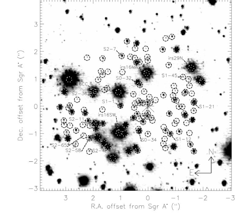
Figure 1.— Identification of sources from this study overlaid on a 6^′′ x 6^′′ region of an LGS K^′-band ($\lambda_{o}$ = 2.1µm) image from Ghez et al. (2006) taken on June 30, 2005. All 131 sources are circled, but only variable sources are labeled. The location of Sgr A^∗ is marked with an asterisk.

Figure 2.— A $m_{K}$ histogram of the 131 stars in our sample which range in magnitude from 9.0 to 16.1 mag.

Photometric zeropoints are established on the basis of the work done by Blum et al. (1996a). While we share 7 stars in common with Blum et al. (1996a) (IRS 16NW, 16SW, 16C, 16NE, 29N, 29S, and 16CC), only IRS 16C ($m_{K}=9.83\pm 0.05$ mag) is a suitable photometric reference source. IRS 16SW is a known variable star in the K-band (Ott et al., 1999; DePoy et al., 2004) and IRS 29N is noted as possibly variable in Hornstein et al. (2002). IRS 16CC appears to be variable in the L-band; Blum et al. (1996a) list a re-calibrated value from Depoy & Sharp (1991) of $8.7\pm 0.2$ mag, while Simons & Becklin (1996) measure $10.2\pm 0.2$ mag. Among the remaining sources, only IRS 16C is in the final source lists of all the images. Several non-variable sources (see §3.2.1) are used a posteriori to confirm that IRS 16C is non-varying. Specifically, we check for any systematic shifts in the zero points by examining the normalized flux densities ($Q_{j}=\sum_{i}^{N}\frac{Flux_{i,j}}{NFlux_{avg_{i}}}$ where index i represents each star in an image of epoch j, $Flux_{avg_{i}}$ is the weighted average of the flux for that star over all images, and N is the number of stars used) of the 7 least variable bright stars that are identified in all 50 images (S1-3, S1-5, S2-22, S2-5, S1-68, S0-13, and S1-25) (see §3.2.1). The photometric stability of IRS 16C is shown in Figure 3, which plots $Q_{j}$ versus the observing dates. The reference source IRS 16C appears to be stable over time, since the standard deviation of $Q_{j}$ is 0.05, which is consistent with our measurement uncertainty for bright stars. Increasing the number of reference stars to 11 non-variable sources present in all frames in all 50 nights yields the same result. We therefore conclude that IRS 16C is non-varying to within our measurement uncertainties, and include it in our list of non-varying sources. Uncertainty in each of our reported relative photometry values is initially estimated as the root mean square (RMS) deviation from the average of the measurements from the three different subset images. The RMS value is added in quadrature with the uncertainty in the brightness of IRS 16C (0.05 mag) determined from the standard deviation of the normalized flux densities $Q_{j}$. As Figure 4 shows, the median uncertainties grow from a floor of about 0.06 mag to 0.21 mag for the K= 16 mag sources.

Figure 3.— The average normalized flux densities ($Q_{j}$, as defined in §3.1) as a function of time. The variations seen are consistent with the measurement uncertainties for bright stars and are therefore demonstrative of the stability of our calibrator IRS 16C. This quantity is used as a scale factor to improve the quality of our relative photometry.

Figure 4.— The median measurement uncertainty of stars binned by magnitude. The median uncertainties grow from a floor of about 0.06 mag to 0.21 mag for the K= 16 mag sources.

3.2. Variability

3.2.1 Identifying Variables

There is a wide range of methods for testing photometric variability and the challenge for these various approaches is to avoid declaring a non-variable source variable on the basis of a few outlying data points (Welch & Stetson, 1993). We therefore have chosen to use the Kolmogorov-Smirnov (KS) test to calculate the probability that a distribution of data points is consistent with a model of a distribution of measurements for a non-variable source. This approach is less sensitive to outlying data points than the commonly used $\chi^{2}$ test, which is an analysis of a single number description of how well a data set matches a model. In the KS test, we adopt as our model a non-variable light curve with gaussian-distributed uncertainties and we test the consistency of the measurements with the model. Specifically, we examine the distribution of $X_{j}=\frac{Flux_{j}-Flux_{avg}}{\sigma_{Flux_{j}}}$ where $Flux_{j}$ is the flux of a star in a image of epoch j, $\sigma_{Flux_{j}}$ is the corresponding uncertainty, and $Flux_{avg}$ is the weighted average of the flux for that star over all images. The resulting KS probabilities, which have allowed values between 0 and 1, describe how likely it is that a source’s measurements are consistent with a non-variable source. Therefore variable stars, whose intensity variations are larger or comparable to our measurement uncertainties, should have very low KS probabilities. We classify a star as variable if it has a KS probability of less than $2.7\times 10^{-3}$, which is the equivalent to a $3\sigma$ cut for gaussian distributed uncertainties (see Figure 5). To ensure all our low KS probability stars are truly variable, we also require these stars to have positive estimates of their intrinsic flux density variance, $\sigma^{2}_{intrinsic}=\sigma^{2}_{measured}-\langle\delta\rangle^{2}$, where the first term is the dispersion of the measured flux densities and the second term removes the bias introduced by the measurement uncertainties, $\delta$. At this point, the 7 least variable bright stars detected in all images, used in §3.1 to define $Q_{j}$, are identified. We then scale all our photometry by $Q_{j}$ in order to reduce the fluctuations induced by measurement errors on IRS 16C. The KS and intrinsic variance tests are then repeated. Table 2 and 3 list the properties of the variable and non-variable stars in our sample, respectively, and the light curves of all variable stars and a few key non-variable stars are shown below in Figures 9, 10, 11, 12, 13, and 15. While there are almost certainly other variable stars that we have excluded, our uncertainties limit our ability to classify more of these stars as variable, especially at the fainter end.

Figure 5.— KS test probabilities of all the stars, with low values implying a low probability for a star to be non-variable. We classify a star as variable if it has a KS probability of less than $2.7\times 10^{-3}$, which is equivalent to a $3\sigma$ cutoff value for gaussian distributed uncertainties and is marked by the dashed line. To ensure all our low KS probability stars are truly variable, we require all variable stars to have positive intrinsic variance. We mark all variable stars identified in this survey with hatches.

Among the 131 stars in our sample, 15 are identified as photometric variables in K-band (see Figure 1). To this we also add IRS 16CC, known to be variable in the L-band (see §3.1). Since the relative photometric uncertainties are roughly uniform down to a $m_{K}$ magnitude of $\sim$ 14 and then grow at fainter magnitudes (see Figure 4), we report a frequency of variable stars based on the stars brighter than 14 mag. Within this brighter sample of 44 stars, there are 10 variable stars, suggesting a minimum frequency of variable stars of 23%. There is no evidence for radial dependence, suggesting that we are not limited by stellar confusion down to 14 mag.

We compare our results to those of Ott et al. (1999), the only other high spatial resolution study of the variability of sources in the Galactic center. Those authors give an upper limit of possible variable stars of approximately 50% of their 218 sources with $m_{K}$ $<$ 13 mag over 18^′′ $\times$ 18^′′. While this variable star frequency is higher than our reported value (and consistent), a comparison limited to the stars in common leads to a number of discrepancies. In the overlap sample of 33 stars, Ott et al. find 2 of the stars to be variable (IRS 16SW, S1-3), while our sample has 6 (IRS 16SW, IRS 16NW, IRS 29N, S2-11, S2-4, S1-21) and only IRS 16SW is in common. There are a number of differences between these two studies, including the data analysis approach used (PSF fitting vs.

Table 2List of Variable Stars

Star ID	Other ID	K	Int. Var.	p	$\Delta$R.A.	$\Delta$Dec.	Probability	Nights	Type
		(mag)	(mag)	(arcsec)	(arcsec)	(arcsec)		(days)
IRS16SW	E23	10.06$\pm$0.19	0.17	1.41	1.04	-0.95	2.3E-23	50	Ofpe/WN9
IRS16NW	E19	10.09$\pm$0.09	0.07	1.21	-0.01	1.21	3.3E-05	49	Ofpe/WN9
IRS29N	E31	10.33$\pm$0.20	0.18	2.15	-1.63	1.40	1.1E-15	35	WC9
IRS16CC	E27	10.60$\pm$0.05	0.01	2.07	1.99	0.57	3.0E-01	50	O9.5-B0.5 I
S2-11	GEN+2.03-0.63	11.99$\pm$0.13	0.11	2.07	1.99	-0.58	4.9E-19	49	Late
S2-4	E28:GEN+1.46-1.49	12.26$\pm$0.17	0.15	2.05	1.45	-1.45	6.1E-14	47	B0-0.5 I
S1-1	GEN+1.01+0.02	13.00$\pm$0.11	0.08	0.98	0.98	0.05	3.6E-04	49	Early
S2-36	$\cdots$	13.28$\pm$0.13	0.12	2.08	2.04	0.43	3.7E-09	48	Early
S1-21	E24:W7	13.33$\pm$0.17	0.15	1.69	-1.69	0.13	4.2E-06	42	O9-9.5 III?
S1-12	E21:W13	13.82$\pm$0.18	0.17	1.31	-0.85	-1.00	4.2E-07	45	OB I?
S2-7	E29:GEN+1.06+1.81	14.06$\pm$0.25	0.21	2.09	0.97	1.85	4.2E-10	45	O9-B0
S0-32	$\cdots$	14.18$\pm$0.20	0.15	0.81	0.26	0.77	6.3E-04	49	Early
S2-58	$\cdots$	14.21$\pm$0.14	0.10	2.45	2.17	-1.14	6.8E-04	47	Early
S1-45	$\cdots$	15.41$\pm$0.55	0.28	1.63	-1.28	1.00	6.1E-06	41	Early
S2-65	$\cdots$	15.83$\pm$0.49	0.29	2.57	2.37	-1.00	2.5E-04	29	$\cdots$
S0-34	$\cdots$	15.85$\pm$0.40	0.31	0.83	0.32	-0.77	4.1E-06	26	$\cdots$

Note. — Photometry is relative to IRS 16C ($m_{k}$=9.83 mag). Positions are in arcseconds offset from Sgr A* in 1999.56 and p is the projected distance. The K-S probability is equal to 1 for an ideal non variable source, and approaches 0 for a very variable source. Other ID’s are from Paumard et al. (2006) and Genzel et al. (2000) respectively. We classify IRS 29N as an early type star according to Paumard et al. (2006) although Figer et al. (2003) classifies it as a late type star.

Table 3List of Non-variable Stars

Star ID	Other ID	K	p	$\Delta$R.A.	$\Delta$Dec.	Nights	Type
		(mag)	(arcsec)	(arcsec)	(arcsec)	(days)
IRS16NE	E39	9.00$\pm$0.05	3.06	2.85	1.10	35	Ofpe/WN9
IRS16C	E20	9.83$\pm$0.05	1.23	1.13	0.50	50	Ofpe/WN9
S2-17	E34:GEN+1.27-1.87	10.90$\pm$0.07	2.23	1.27	-1.84	35	B0.5-1 I
IRS16SW-E	E32:16SE1	11.00$\pm$0.08	2.15	1.85	-1.11	50	WC8/9
IRS29S	$\cdots$	11.31$\pm$0.06	2.08	-1.86	0.93	30	K3 III
S1-24	E26:GEN+0.76-1.55	11.64$\pm$0.07	1.72	0.73	-1.55	45	O8-9.5 I
S2-16	E35:29NE1	11.85$\pm$0.08	2.29	-1.01	2.05	33	WC8/9
S1-23	GEN-0.90-1.46	11.86$\pm$0.09	1.73	-0.92	-1.46	33	Late
S3-2	GEN+3.07+0.56	12.00$\pm$0.11	3.09	3.03	0.60	31	Early
S2-6	E30:GEN+1.60-1.36	12.06$\pm$0.08	2.07	1.59	-1.31	50	O8.5-9.5 I
S1-3	E15:GEN+0.57+0.84	12.10$\pm$0.06	0.99	0.46	0.88	50	Early
S3-5	E40:16SE	12.15$\pm$0.09	3.16	2.95	-1.13	21	WN5/6
S2-8	W2	12.24$\pm$0.08	2.16	-1.99	0.84	23	Early
S1-17	GEN+0.55-1.45	12.51$\pm$0.08	1.52	0.50	-1.44	49	Late
S1-4	GEN+0.77-0.71	12.53$\pm$0.07	1.02	0.77	-0.66	50	Early
S2-19	E36:GEN+0.53+2.27	12.62$\pm$0.11	2.34	0.42	2.30	33	O9-B0 I?
S1-20	GEN+0.41+1.59	12.70$\pm$0.11	1.66	0.37	1.61	49	Late
S1-22	E25:W14	12.72$\pm$0.08	1.72	-1.65	-0.51	42	O8.5-9.5 I?
S1-5	GEN+0.43-0.96	12.78$\pm$0.04	0.98	0.37	-0.91	50	Late
S1-14	E22:W10	12.82$\pm$0.07	1.40	-1.37	-0.30	46	O8-9.5 III/I
S3-6	GEN+3.26+0.08	12.82$\pm$0.05	3.22	3.22	0.09	17	Late
S2-22	GEN+2.37-0.29	12.92$\pm$0.04	2.33	2.32	-0.22	50	Late
S2-38	$\cdots$	12.93$\pm$0.09	2.12	2.04	0.58	44	Late
S2-31	GEN+2.91-0.20	13.06$\pm$0.10	2.84	2.83	-0.15	42	Late
S1-34	$\cdots$	13.20$\pm$0.14	1.29	0.86	-0.96	50	$\cdots$
S2-5	GEN+1.91-0.86	13.32$\pm$0.05	2.05	1.89	-0.80	50	Early
S1-68	$\cdots$	13.38$\pm$0.06	1.97	1.89	-0.55	50	$\cdots$
S2-21	GEN-1.70-1.65	13.47$\pm$0.10	2.36	-1.70	-1.65	12	Early
S0-13	GEN+0.59-0.47	13.49$\pm$0.04	0.69	0.54	-0.42	50	Late
S1-25	GEN+1.69-0.66	13.54$\pm$0.05	1.76	1.65	-0.60	50	Late
S2-26	$\cdots$	13.60$\pm$0.13	2.56	0.69	2.47	20	Late
S0-15	E16:W5	13.70$\pm$0.07	0.98	-0.93	0.29	48	O9-9.5 V
S0-14	E14:W9	13.72$\pm$0.08	0.83	-0.78	-0.27	50	O9.5-B2 V
S1-19	GEN+0.38-1.58	13.82$\pm$0.12	1.62	0.36	-1.58	46	Early
S2-2	GEN-0.54+2.00	14.07$\pm$0.11	2.12	-0.59	2.03	41	Late
S0-2	E1:S2	14.16$\pm$0.08	0.12	-0.07	0.10	33	B0-2 V
S1-8	E18:W11	14.19$\pm$0.11	1.08	-0.67	-0.85	49	OB
S1-15	W4	14.21$\pm$0.10	1.46	-1.37	0.52	47	Late
S0-6	S10	14.26$\pm$0.09	0.39	0.07	-0.38	49	Late
S1-49	$\cdots$	14.26$\pm$0.13	1.66	-1.65	0.15	23	$\cdots$
S1-13	W12	14.27$\pm$0.12	1.42	-1.10	-0.90	46	Early
S2-47	$\cdots$	14.29$\pm$0.08	2.26	2.20	-0.49	48	Early
S0-9	S11	14.31$\pm$0.08	0.55	0.14	-0.53	49	Early
S0-12	W6	14.38$\pm$0.06	0.68	-0.57	0.37	49	Late
S2-3	W15	14.48$\pm$0.09	2.09	-1.54	-1.41	23	Late
S0-4	E10:S8	14.49$\pm$0.11	0.37	0.32	-0.19	49	B0-2 V
S0-3	E6:S4	14.50$\pm$0.14	0.25	0.22	0.13	19	B0-2 V
S2-75	$\cdots$	14.52$\pm$0.12	2.78	2.65	-0.85	40	$\cdots$
S2-69	$\cdots$	14.57$\pm$0.14	2.64	-0.91	2.48	13	Early
S3-4	$\cdots$	14.61$\pm$0.20	3.14	3.10	-0.47	20	Early
S0-1	E4:S1	14.67$\pm$0.11	0.14	-0.11	-0.09	49	B0-2 V
S2-23	$\cdots$	14.72$\pm$0.13	2.43	1.64	1.80	39	Late
S1-55	$\cdots$	14.80$\pm$0.39	1.69	1.58	0.59	41	$\cdots$
S1-50	$\cdots$	14.82$\pm$0.37	1.67	1.51	0.72	41	$\cdots$
S1-52	$\cdots$	14.83$\pm$0.29	1.66	-0.02	1.66	42	$\cdots$
S1-10	W8	14.88$\pm$0.12	1.15	-1.15	-0.04	42	$\cdots$
S1-2	E17:GEN-0.06-1.01	14.90$\pm$0.12	1.00	-0.05	-1.00	45	Early
S1-33	$\cdots$	15.01$\pm$0.10	1.25	-1.24	-0.07	40	$\cdots$
S1-58	$\cdots$	15.04$\pm$0.35	1.77	-1.48	0.98	37	$\cdots$
S1-51	$\cdots$	15.05$\pm$0.15	1.66	-1.65	-0.20	39	Early
S2-86	$\cdots$	15.05$\pm$0.23	2.99	2.68	-1.33	24	Early
S3-3	$\cdots$	15.06$\pm$0.33	3.12	3.06	-0.62	19	Early
S2-30	$\cdots$	15.13$\pm$0.19	2.88	2.88	0.00	23	$\cdots$
S1-18	$\cdots$	15.14$\pm$0.15	1.66	-0.73	1.49	39	Early
S0-5	E9:S9	15.17$\pm$0.16	0.36	0.18	-0.31	43	B0-2 V
S0-31	E13	15.20$\pm$0.23	0.66	0.49	0.45	40	B V
S2-34	$\cdots$	15.21$\pm$0.22	2.04	1.79	0.98	43	$\cdots$
S0-26	E8:S5	15.27$\pm$0.22	0.39	0.36	0.16	40	B4-9 V
S1-44	$\cdots$	15.28$\pm$0.41	1.61	0.26	1.59	40	$\cdots$
S3-16	$\cdots$	15.30$\pm$0.20	3.15	3.02	-0.88	14	Late
S2-82	$\cdots$	15.30$\pm$0.29	2.88	2.87	0.08	27	Late
S2-12	$\cdots$	15.33$\pm$0.17	2.07	1.68	1.22	38	Late
S1-32	$\cdots$	15.33$\pm$0.13	1.13	-0.93	-0.64	42	$\cdots$
S1-39	$\cdots$	15.35$\pm$0.16	1.45	-0.53	-1.35	30	Early
S0-11	E12:S7	15.36$\pm$0.13	0.53	0.53	-0.01	40	B V
S0-18	S18	15.36$\pm$0.13	0.43	-0.09	-0.42	45	$\cdots$
S1-35	$\cdots$	15.36$\pm$0.19	1.27	-1.24	-0.25	38	$\cdots$
S2-63	$\cdots$	15.39$\pm$0.28	2.56	-0.69	2.47	16	Early
S1-54	$\cdots$	15.41$\pm$0.23	1.68	-1.53	0.70	36	$\cdots$
S1-62	$\cdots$	15.41$\pm$0.31	1.82	0.51	1.74	37	$\cdots$
S1-53	$\cdots$	15.44$\pm$0.15	1.68	1.68	-0.09	30	$\cdots$
S2-61	$\cdots$	15.46$\pm$0.17	2.54	2.46	-0.64	38	$\cdots$
S2-46	$\cdots$	15.47$\pm$0.30	2.18	2.08	-0.64	38	$\cdots$
S2-73	$\cdots$	15.50$\pm$0.32	2.72	2.21	-1.58	29	$\cdots$
S1-6	$\cdots$	15.54$\pm$0.13	1.15	-0.91	0.71	34	Early
S1-48	$\cdots$	15.54$\pm$0.23	1.62	-0.60	-1.50	22	$\cdots$
S0-7	E11:S6	15.55$\pm$0.27	0.45	0.44	0.11	35	B V
S0-19	E5	15.56$\pm$0.19	0.19	-0.09	0.17	28	B4-9 V
S1-64	$\cdots$	15.57$\pm$0.36	1.91	0.60	1.81	34	$\cdots$
S2-80	$\cdots$	15.57$\pm$0.27	2.86	2.22	1.80	20	Early
S2-40	$\cdots$	15.58$\pm$0.18	2.15	1.68	1.34	35	Early
S2-42	$\cdots$	15.61$\pm$0.28	2.11	0.41	2.07	26	$\cdots$
S1-27	$\cdots$	15.62$\pm$0.27	1.09	-1.07	0.24	39	$\cdots$
S1-26	$\cdots$	15.62$\pm$0.13	1.02	-0.95	0.38	40	$\cdots$
S1-37	$\cdots$	15.63$\pm$0.16	1.42	-1.34	0.47	36	$\cdots$
S1-47	$\cdots$	15.67$\pm$0.23	1.63	-1.57	0.45	34	$\cdots$
S0-16	E2	15.68$\pm$0.19	0.08	0.05	0.06	18	B4-9 V
S1-59	$\cdots$	15.70$\pm$0.25	1.86	0.01	1.86	27	$\cdots$
S1-31	GEN-0.91+0.44	15.70$\pm$0.18	1.14	-0.99	0.57	31	$\cdots$
S0-29	$\cdots$	15.72$\pm$0.50	0.54	0.25	-0.48	21	$\cdots$
S2-83	$\cdots$	15.74$\pm$0.19	2.94	2.87	-0.63	16	$\cdots$
S0-27	$\cdots$	15.74$\pm$0.18	0.54	0.13	0.52	32	$\cdots$
S1-36	$\cdots$	15.75$\pm$0.27	1.36	-0.67	-1.18	30	$\cdots$
S2-37	$\cdots$	15.77$\pm$0.31	2.11	0.04	2.11	29	$\cdots$
S0-8	E7	15.79$\pm$0.14	0.47	-0.32	0.34	29	B4-9 V
S1-7	$\cdots$	15.81$\pm$0.14	1.12	-1.00	-0.50	34	$\cdots$
S1-65	$\cdots$	15.82$\pm$0.15	1.93	1.43	1.29	31	Early
S0-28	S19	15.85$\pm$0.18	0.61	-0.18	-0.58	30	$\cdots$
S2-64	$\cdots$	15.85$\pm$0.59	2.56	2.54	0.31	16	$\cdots$
S0-36	$\cdots$	15.85$\pm$0.28	1.03	-0.60	-0.84	29	$\cdots$
S0-20	E3	15.86$\pm$0.20	0.21	-0.18	-0.10	33	B4-9 V
S1-40	$\cdots$	15.95$\pm$0.23	1.50	-1.36	-0.64	26	$\cdots$
S1-61	$\cdots$	15.99$\pm$0.38	1.76	-1.43	-1.03	21	$\cdots$
S2-52	$\cdots$	16.02$\pm$0.20	2.37	2.37	-0.07	21	$\cdots$
S1-42	$\cdots$	16.13$\pm$0.22	1.60	0.94	1.29	19	$\cdots$

Note. — See notes from table 1.

aperture photometry), the time baseline (10 years vs. 5 years), and the angular resolution (0$\farcs$05 vs. 0$\farcs$13 ). Since our study covers twice the time baseline, we can pick out variations on longer time scales, which helps explain our additional variables. Also, the high stellar crowding makes the area we observe the most uncertain region for the lower resolution Ott et al. study. Only one star, S1-3, in our non-variable sample is identified as variable by Ott et al., and it is very close to their threshold for variability.

Figure 6.— Determination of IRS 16SW’s period using Dworetsky’s string length method Dworetsky (1983). Phi is the string length where shorter lengths and therefore smaller values of Phi indicate a periodic signal. Note that the other harmonics are also found at multiples of the original period.

Figure 7.— The phased light curve of IRS 16SW at its period of 9.724 (top panel) and 19.448 days (bottom panel). The points are plotted twice for clarity. Both phased diagrams show a rise-time that is $\sim 1.6$ times longer than the fall-time. The similarity of the first half of the data set (1995-2000; diamonds) to the second half (2001-2005; crosses) shows that the asymmetry has been constant over the past ten years. This effect could be produced by tidal deformation of two equal mass stars in an eclipsing binary star system.

3.2.2 Variability Characterization and Periodicity Search

We attempt to characterize the minimum time-scale for variation by searching for daily and monthly variability using KS tests similar to the test for variability in §3.2.1 where we adopt as our model a non-variable light curve with gaussian-distributed uncertainties. For the daily variations, we group the consecutive nights in pairs and examine the distribution of the pairs in sets $i$ for each star of $X_{i}=\frac{Flux_{j}-Flux_{k}}{\sqrt{\sigma_{Flux_{j}}^{2}+\sigma_{Flux_{k}}^{2}}}$ where $Flux_{j}$ and $Flux_{k}$ are the fluxes of stars in images of consecutive epochs j and k respectively, $\sigma_{Flux_{j}}$ and $\sigma_{Flux_{k}}$ are the corresponding uncertainties. For the monthly variation, all measurements made within days of each other are averaged together and the pairs separated by one month are examined with the same KS test. The only stars showing daily variability in excess of $3\sigma$ is IRS 16SW, and the stars showing monthly variations are IRS 16SW and S2-36.

The light curves of the variable stars are searched for periodicities using three different methods. First, the Lomb and Scargle periodogram technique (Lomb, 1976; Scargle, 1982; Press et al, 1992), which fits fourier components to the data points, is applied and is expected to yield a larger power spectral density at intrinsic harmonics of a data set in which there is a periodic signal. Second, Dworetsky’s (1983) string length method, a variant of the Lafler-Kinman method (1965), phases the data for every possible period and then sums over the total separation between points in phase space, with the best period and its aliases corresponding to the smallest lengths. Third, Stetson’s (1996) string length technique is similar to Dworetsky’s, but also weights these lengths by their uncertainties and how close in phase the points are. Our criterion for considering a star periodic is that it show similar periods from all three techniques. The periodicity search shows only one periodic star: IRS 16SW. We find a photometric period of $9.724\pm 0.001$ days, which is consistent with Ott et al. (1999), DePoy et al. (2004) and the reanalysis of the Ott et al. data in Martins et al. (2006). Figure 6 shows the determination of IRS 16SW’s period using Dworetsky’s (1983) string length algorithm, showing the 9.724 day period and its other harmonics at multiples of its period. The top panel in Figure 7 shows the phased light curve of IRS 16SW at 9.724 days and depicts a clearly periodic signal with an amplitude of $\sim 0.55$ mag. The phased light curve of IRS 16SW is asymmetric (see Figure 7) with a rise-time that is $\sim 1.6$ times longer than the fall-time.

Figure 8.— Apparent K magnitudes versus spectral type assuming a distance of $r=8.0$ kpc (Reid, 1993) and an extinction $A_{K}$=3.3 mag (Blum et al., 1996a) based on compilations of data from Cox (2000) where available, and by (de Jager & Nieuwenhuijzen, 1987; Wegner, 1994, 2006; Vacca et al., 1996; Grenier et al., 1985; Blackwell & Lynas-Gray, 1994; Theodossiou & Danezis, 1991) for Giants of type O-F . The lower dotted line is the magnitude limit of this sample, and the locations of WR and LBV stars are highly variable and average locations are marked for reference only. The triangles represent supergiant stars, the crosses represent giant stars, and the diamonds represent main sequence stars.

4. Discussion

The 16 variable stars identified in this study cover a wide variety of different types of stars, as we only limited our search by location and brightness. As Figure 8 shows, based on the K magnitudes alone, this sample is expected to contain early-type (O & B) main sequence stars, late-type (K & M) giant stars, and most types of supergiants. Fortunately, all but two of the variable stars have spectral classifications (see column 10 in Table 2). While 9 of the variable stars are securely identified from spectroscopic work (Paumard et al., 2006; Eisenhauer et al., 2005; Figer et al., 2003; Ott, 2003), an additional 5 stars are classified on the basis of narrowband photometry of CO absorption (Ott, 2003; Genzel et al., 2003). In summary, four stars are LBV candidates (IRS 16SW, 16NW, 16NE, & 16C; see §4.1) one is a WC9 (IRS 29N; see §4.2), four are OB supergiants (S2-4, S1-12, S2-7, & IRS 16CC; see §4.3), one is an O giant (S1-21), five more are classified as some sort of early-type star from narrowband filter photometric measurements (S1-1, S2-36, S0-32, S2-58, S1-45), and one is classified as a late-type star from narrowband filter photometric measurements (S2-11; see §4.3). The variability of stars in each spectral classification is discussed in turn below, along with a discussion of the possibility of external agents causing variability.

4.1. Ofpe/WN9 Stars

4.1.1 Luminous Blue Variable Candidates

Four stars in our sample are Ofpe/WN9 stars and have been previously classified as candidate LBVs (IRS 16NE, 16C, 16SW, and 16NW) based on their bright luminosity, their narrow emission lines, and their proximity and similarity to IRS 34W (Clark et al., 2005; Paumard et al., 2004b; Trippe et al., 2006) . In our observations, both IRS 16NE and 16C are non-variable over a ten-year time frame to within our uncertainties. The other two LBV candidates (IRS 16NW and 16SW) show variability, but not the characteristic LBV eruptions, which in the context of this study are the $\Delta M_{v}\simeq 1-2$ mag events occurring every 10-40 years and lasting as long as several years (Humphreys & Davidson, 1994). IRS 16SW has periodic variability that is explained by an eclipsing binary system (see §4.1.2 below) and IRS 16NW has an overall flat light curve with a decrease in brightness ($\Delta m_{K}\simeq 0.2$) mag between 1997 and 1999 (see Figure 9). The apparent dimming of IRS 16NW can be explained by ejected circumstellar material obscuring the star, with an amplitude that is smaller than is characteristic of a typical LBV. These variations do not require it to be an LBV, just that it has strong stochastic winds. While none of these stars shows the classic characteristics of LBVs, our time baseline is too short to rule them out as LBVs as they may be in a quiescent phase. Nonetheless, our observations do not demand the complication of multiple recent star formation events that would be suggested with the presence of both LBVs and WR stars.

Figure 9.— Light curves of the four stars in our sample that are classified as candidate LBVs (IRS 16SW, 16NW, 16NE, 16C). The top two panels denote the two variable stars, while the bottom two panels are non-variable stars. The given intrinsic variance is in magnitudes.

4.1.2 Asymmetric Periodic Light Variations in IRS 16SW: Tidal Deformation?

The periodic variation in IRS 16SW has recently been attributed to either an equal mass contact eclipsing-binary or a massive pulsating star (Ott et al., 1999; DePoy et al., 2004; Martins et al., 2006), although the measurement of a spectroscopic radial velocity period by Martins et al. (2006) strongly suggests it is an eclipsing binary star system. Also, a re-analysis of the data suggesting a pulsating star now agrees with IRS 16SW probably being an eclipsing binary (Peeples et al., 2006). The asymmetries that we observe in the phased light curve of IRS 16SW are difficult to explain in the context of an eclipsing binary star system. Figure 7 shows the properly phased light curve ($19.448\pm 0.002$ days), in which asymmetries in its rise and fall-times are still readily detected. The asymmetry is remarkably similar for both halves of the phased light curve. While this was not detected in earlier photometric studies, our study is likely more sensitive to small photometric variations due to our higher angular resolution (see §3.2.1). The observed asymmetry has been sustained over 10 years; if the asymmetry has been changing over time, it would show up as a dispersion in the vertical placements of the points in the phase diagram that is much larger than what we observe. In figure 7 we explicitly show that the asymmetries are the same during the first half and second half of the data-set and we see no period drifts, with the period of the first half and second half not differing at the $3\sigma$ confidence level. Magnetic hot spots can explain light curve asymmetries (Djurašević et al., 2000; Cohen et al., 2004), however, they can not maintain this asymmetry over long periods of time. Furthermore, the similarity in the asymmetry between the first and second half would require the spots to be the same on both stars. Likewise, heating in the contact region of the binary or any third light in this region produces a light curve that is a mirror reflection between the 1st and 2nd half (see Moffat et al., 2004) and is therefore inconsistent with our observations. Other heating mechanisms such as irradiation effects are unlikely to be the cause of the asymmetry as they barely change the light curve (Bauer, 2005). Given that this is suspected to be a contact binary, we suggest that the asymmetric light curve may be due to tidal deformations caused by the proximity of the stars in asynchronous orbits. Since these two stars are equal in mass ($\sim 50M_{\odot}$), equal in radius ($66R_{\odot}$) and appear to be in contact (Martins et al., 2006), they fall within the tidal radius of $\sim 163R_{\odot}$, and are likely tidally deformed. In order to produce the asymmetric light curve, the rotation of the stars needs to be asynchronous with their orbital periods so that the rotational inertia of the stars prevents their tidal bulges from being aligned with the line joining the stars’ centers of mass. Two stars in such close contact will eventually synchronize their orbital period with their rotation period. The synchronization time scale of stars with convective cores and radiative envelopes is longer than for stars with convective envelopes, albeit more difficult to calculate (Zahn, 1977). We therefore calculate the convective envelope synchronization time as a minimum time for synchronization based on formalism developed by Zahn (1977) and find a minimum age of $\sim 6\times 10^{8}$ yrs. This time scale is far larger than the lifetime of stars as massive as IRS 16SW and asynchronous orbits are therefore acceptable. The equality of the two halves of the light curve implies that the rotation rate of the two stars is very similar. Since these two stars are identical in every other respect, this equality is not surprising. It is therefore possible that the asymmetric light curve is due to tidal deformations.

4.1.3 Eclipsing Binary Fraction

Stars close to the Galactic center are expected to have a higher fraction of ellipsoidal and eclipsing variable binaries than the stars in the solar neighborhood. However, IRS 16SW is the only eclipsing binary star detected in our sample. The stars’ orbits may be smaller due to hardening by encounters with other stars producing tightly bound binaries, such that eclipses would be more likely. In addition, collisions and tidal capture produce binaries, making ellipsoidal variations or eclipses more probable (Tamura et al., 1999). Of the 164 Galactic O stars in clusters or associations in the sample by Mason et al. (1998), 50 are confirmed as spectroscopic binaries, 40 are unconfirmed spectroscopic binaries, 4 are confirmed eclipsing variables, and 14 are either ellipsoidal or eclipsing binaries. This yields local rates of eclipsing O star binaries between 2% and 11%. Our sample contains 11 spectroscopically confirmed O stars, 4 Ofpe/WN9 stars, and possibly more unconfirmed. If the Galactic center fraction of eclipsing binaries is similar to the cluster results, we would expect on the order of one eclipsing binary. Our detection of one eclipsing variable star suggests that the frequency of eclipsing binaries is not significantly increased at the Galactic center over the local neighborhood.

Figure 10.— Light curves of Wolf-Rayet stars of type WC in our sample. The first panel is the variable star IRS 29N, which is probably a wind-colliding binary, while the other two are non-variable stars. The given intrinsic variance is expressed in magnitudes.

4.2. Late-type WC Wolf-Rayet Stars: Variations Associated with a Wind Colliding Binary

Three stars in our sample are spectroscopically identified as WC stars (IRS 29N, IRS 16SW-E and S2-16) (Paumard et al., 2006), and all three are dust producers as evidenced by their red colors (K-L $\sim 3$; Blum et al. 1996a, Wright et al. 2006). In this study, only IRS 29N is variable (see Fig 10). IRS 29N’s intensity shows a gradual drop and then rise in brightness of $\Delta m_{K}\simeq 0.7$ mag over a time scale of $\approx 5$ years. Its light curve is similar to the variations seen in WC stars elsewhere in the Galaxy (e.g. compilation by van der Hucht et al. 2001b); these sources are thought to be variable due to periodic or episodic dust production in the wind collision zone of long period eccentric binary star systems (1000d $<$ P $<$ 10000d) during periastron passage. When the dust forms, the star exhibits a rising infrared flux followed by fading emission when dust formation stops and dust grains are dispersed by stellar winds (Moffat et al., 1987; White & Becker, 1995; Veen et al., 1998; Williams & van der Hucht, 1992, 2000). Currently, only seven WC stars have been observed to produce dust episodically, all of which are confirmed or suspected massive binaries with elliptical orbits (van der Hucht, 2001a; Williams et al., 2005; Lefèvre et al., 2005). Two of these are known to exhibit pinwheel nebulae, a tell-tale sign of wind-colliding binaries (Tuthill et al., 1999; Monnier et al., 1999). The time-scales and magnitude of the photometric variability of IRS 29N is consistent with it being a wind-colliding binary; we therefore conclude that IRS 29N is likely to be a wind-colliding binary.

Figure 11.— Light curves of variable OB stars in our sample. IRS 16CC is not variable in K band, but shows variability at L (see §3.1). We propose that S2-4 and S1-12 are variable due to ejection of circumstellar material obscuring the stars, while S2-7 is probably a Be star with the formation of an equatorial disk obscuring the star. The given intrinsic variance is expressed in magnitudes.

Figure 12.— Light curves of early-type variable stars in our sample. S2-36 is variable on a monthly basis and its variation is therefore probably intrinsic. The variations in S1-45 and S2-58 may be due to obscuration by high density streamers. The given intrinsic variance is expressed in magnitudes.

4.3. Comments on Other Stars

Our sample includes at least 10 other variable young massive stars in addition to those discussed in §4.1 & §4.2. Five are spectroscopically identified OB stars (IRS 16CC, S2-4, S1-21, S1-12, S2-7; see Figure 11) (Paumard et al., 2006), and five are early-type stars classified as on the basis of narrowband filter photometric measurements (S1-1, S2-36, S0-32, S2-58, S1-45; see Figure 12) (Genzel et al., 2003; Ott, 2003). The majority of these variables are likely associated with mass loss, although interstellar extinction could also play a role, as discussed below. In particular, the two K-band variable OB supergiants each show a dip (0.3 - 0.9 mag) in their brightness that lasts for 1-6 years. OB supergiants have stochastic winds with high mass loss rates ($0.2-20\times 10^{-6}M_{\odot}$/yr) (Massey, 2003); it is therefore likely the large variations seen are due to ejection of circumstellar material. Another example of an OB star with variations potentially due to mass loss is S2-7, which is either luminosity class III or V based on its assumed distance. S2-7 shows a decrease in luminosity between 2000 and 2005 with $\Delta m_{K}\simeq 0.5-1.0$ mag. This is reminiscent of Be stars, which sometimes show fading events due to the formation of an equatorial disk on time scales of several years (Mennickent et al., 1994; Pavlovski et al., 1997; Percy & Bakos, 2001). The remaining young variable stars in our sample have variations that are more difficult to characterize, although S2-36 seems to have significant variations on monthly time-scales (see §3.2.2). Nonetheless, it is likely that mass loss also plays a central role in generating the observed variations.

4.4. Interstellar Material

4.4.1 Apparent Variations Caused by Stellar Motion Through the Line of Sight Extinction

Periods of reduced luminosity in stars can also be due to external effects such as obscuration by foreground interstellar matter. The central parsec has several gas patches that are a few arcseconds wide and that can cause local extinction enhancements of $\sim 1$ magnitude in K-band (Paumard et al., 2004a). As our FOV is only 5$\tt{}^{\prime\prime}\times$5^′′, these patches would cover a sizable region and many neighboring stars would show similar variations. Interstellar material closer to Earth in the line of sight is unlikely, as its proximity would make the clouds even larger in projection (Trippe et al., 2006). Since neighboring stars do not experience similar effects of obscuration, the large scale structure in the interstellar medium (ISM) is unlikely to be the cause.

In some cases it is possible that the variable obscuration is caused by the relative motion of the foreground high density streamers and the background stars, such as are observed in the L-band associated with the Northern Arm (Clénet et al., 2004; Ghez et al., 2005b; Mužič et al., 2006). In this area we see unresolved streamers that are small in projected width ($<80$ mas). These streamers may be due to shocks heating the neighboring dust with the streamers tracing thin shells of compressed gas from one or several shocks (Clénet et al., 2004). These streamers may cause dips in our light curves due to small-scale structure obscuration in the line of sight. This causes photometric variability due to the relative lateral motion between the absorbing feature and the star. The projected implied width of the small-scale structure is approximately $\sim 10-40$ mas assuming a projected stellar velocity of $\sim 5$ mas/yr which is typical of stars at projected distances of $\sim 2\tt^{\prime\prime}$ from Sgr A^∗. The three stars whose variability is most likely ascribable to these thin high density streamers are S2-11, S1-45, S2-58. The most clear case is the late-type star S2-11 (Ott, 2003), which shows an interval of reduced luminosity between 2001 and 2005 with $\Delta m_{K}\simeq 0.3$ mag and is otherwise constant over our time frame (see Figure 13). Using a Galactic center distance of $r=8.0$ kpc (Reid, 1993) and an extinction $A_{K}$=3.3 mag (Blum et al., 1996a) , we determine its spectral type based on luminosity and late-type classification as M3-5 III. Stars with spectral type M5 and luminosity class III are generally classified as asymptotic giant branch stars (AGB), but the variations observed are not typical of AGB stars which have periods between 0.5 - 1.5 yrs (Habing, 1996). This star is likely obscured by dust given its red color (K-L $\sim 2$; Wright et al. 2006). It is located in the middle of the Northern Arm (see Figure 14) and its reduced luminosity is likely due to a high density streamer in the line of sight. The two other stars whose variability can probably be attributed to high density streamers have long term variations over ten years; S1-45 appears to brighten by $\Delta m_{K}\simeq 0.5-1.0$ mag and S2-58 appears to dim by $\Delta m_{K}\simeq 0.2$ mag (see Figure 12). It is also possible that the dips in the light curves of stars speculated to be variable due to high stellar winds such as S2-4, S1-12, S2-7, and S2-36 are actually variable due to obscuration in the line of sight. Measurements at multiple wavelengths throughout future variations would help to establish the role of variable extinction in the observed K-band variations. Furthermore, foreground material would be polarized due to the magnetic fields at the Galactic center, and therefore polarization variations of stars would provide a test of the hypothesis that the relative motion of streamers and stars are responsible for stellar intensity variations.

Figure 13.— Light curves of a late-type star, and two unknown type stars in our sample. The late-type star, S2-11, is probably an AGB star of spectral type M3-5 III, while we are unable to classify the two stars of unknown spectral type. The given intrinsic variance is expressed in magnitudes.

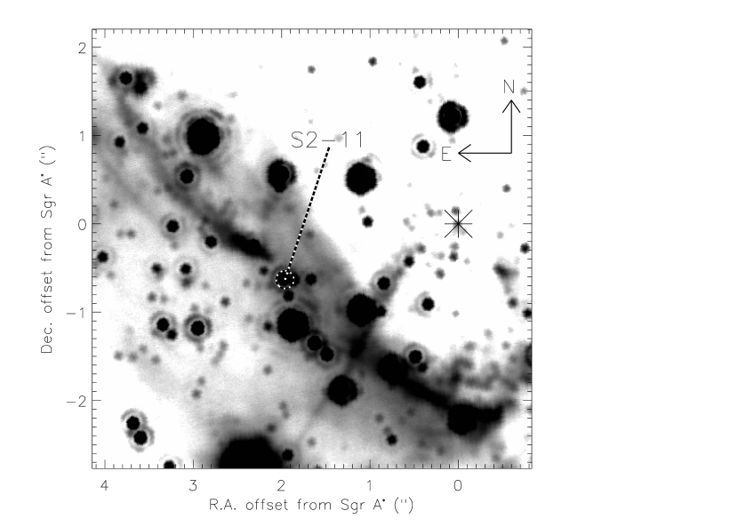
Figure 14.— Identification of the source S2-11 from this study overlaid on a 5^′′ x 5^′′ region of an LGS L^′-band ($\lambda_{o}$ = 3.8µm) image from Ghez et al. (2006) taken on June 30, 2005. The star S2-11 is situated in the middle of the Northern Arm and it is therefore likely that the interval of reduced luminosity is due to the stellar motion through a high density streamer in the line of sight. The location of Sgr A^∗ is marked with an asterisk.

4.4.2 Variability of Stars Near Closest Approach

We detect no variability in the 7 central arcsecond sources that have known 3-dimensional orbits (S0-1, S0-2, S0-4, S0-5, S0-16, S0-19, S0-20) (see Figure 15). The three fainter stars (S0-16, S0-19, S0-20) have missing measurements that are due to insufficient image sensitivity, although they are detected in higher signal-to-noise images made from multiple nights of data (Ghez et al., 2005). The photometry of these stars constrains the properties of a cold, geometrically-thin inactive accretion disk around Sgr A^∗, since in the presence of such a disk we would expect to see nearby stars significantly flaring in the NIR as they passed through and interacted with the disk, and eclipsed at other times. When a nearby star approaches such a disk we would see enhanced NIR flux from reprocessed UV and optical starlight incident on the disk (which we call a flare). Also, we would expect the disk to eclipse the star, reducing the flux from the star in varying amounts depending on the properties of the disk. The time-scales vary based on the geometry of the disk but are on the order of a year and months for the eclipses and flares, respectively (Nayakshin & Sunyaev, 2003; Cuadra et al., 2003). An optically thin disk may not fully eclipse stars, and gaps in our observations would allow different geometries of the disk to account for any one star not showing eclipses or flares as was calculated for S0-2 (Cuadra et al., 2003). However, with the ensemble of stars that we have monitored, the effects of a disk with any orientation should be evident. We constrain the NIR optical depth to be $\lesssim 0.1$. If we assume the NIR standard interstellar dust opacity at 2.2$\micron$ where the dust extinction is approximately $\sim 5\times 10^{-22}cm^{2}$ per hydrogen atom (see Fig. 2 in Voshchinnikov et al. 2003), we find the column density of the disc to be $\sim 2\times 10^{20}cm^{-2}$. However, dust grains may be larger in size or non-existant in the disc (Cuadra et al., 2003; Nayakshin et al., 2004), and such constraints should therefore be approached cautiously. Regardless, the lack of observed flares or eclipses in the 7 central arcsecond sources that have known 3-dimensional orbits puts such severe constrains on the density and size of any possible disc disk around Sgr A^∗ that such a disk is unlikely to exist.

Figure 15.— Light curves of 7 central arcsecond sources that have known 3-dimensional orbits. The X’s mark observations that are rejected due to confusion with other sources, and the boxes are areas where the nightly images have missing measurements due to insufficient image sensitivity and correspond to detections in monthly averaged images. None of these stars are variable, which is evidence against the presence of a dusty disk around Sgr A^∗. The given intrinsic variance is expressed in magnitudes.

5. Summary

We use ten years of diffraction-limited K-band speckle data to determine the photometric stellar variability in the central 5^′′ $\times$ 5^′′ of our Galaxy. Within this study’s limiting magnitude of $m_{K}<16$ mag, we find 15 K-band variable stars out of 131 well-sampled stars. Among 46 stars brighter than $m_{K}<14$ mag with uniform photometric uncertainties, there are 10 variable stars, suggesting a minimum variable star frequency of 23%. We find one periodic star, IRS 16SW, with a period of P=$19.448\pm 0.002$ days, in agreement with Ott et al. (1999), DePoy et al. (2004), and Martins et al. (2006). Our data are consistent with an eclipsing binary and show a rise-time that is $\sim 1.6$ times longer than the fall time and we suggest that the asymmetric light curve results from tidal deformations of the two stars in the presence of asynchronous rotation. We expect to see on the order of one eclipsing binary in our sample for conditions similar to the rest of the Galaxy, suggesting that the frequency of eclipsing binaries is not significantly increased at the Galactic center over the local neighborhood. We identify IRS 29N as a wind colliding binary based on its light curve and spectral classification. This rare object warrants further investigation to confirm its binary nature. None of the IRS 16 stars shows the classic eruptive events of LBVs, although our time baseline is too short to rule them out as LBVs. Among the remaining variable early-type stars in our sample, 3 exhibit large variations on time-scales of a year, which are either due to obscuration from mass loss events or from line of sight extinction variations. Three more stars in our sample exhibit long term variations of $\sim$5-10 yrs probably due to line of sight extinction variations due to high density streamers. Seven stars in the central arcsecond do not show photometric variations indicative of a cold geometrically thin inactive accretion disk which puts such severe constraints on the density and size of any possible disk around Sgr A^∗ that such a disk is unlikely to exist.

References

- Abbott & Conti (1987) Abbott, D. C., & Conti, P. S. 1987, ARA&A, 25, 113
- Bauer (2005) Bauer, M. 2005, Ap&SS, 296, 255
- Blackwell & Lynas-Gray (1994) Blackwell, D. E., & Lynas-Gray, A. E. 1994, A&A, 282, 899
- Blum et al. (1996a) Blum, R. D., Sellgren, K., & DePoy, D. L. 1996a, ApJ, 470, 864
- Blum et al. (1996b) Blum, R. D., Sellgren, K., & Depoy, D. L. 1996b, AJ, 112, 1988
- Blum et al. (2003) Blum, R. D., Ramírez, S. V., Sellgren, K., & Olsen, K. 2003, ApJ, 597, 323
- Christou (1991) Christou, J. C. 1991, PASP, 103, 1040
- Clark et al. (2005) Clark, J. S., Larionov, V. M., & Arkharov, A. 2005, A&A, 435, 239
- Clénet et al. (2004) Clénet, Y., et al. 2004, A&A, 417, L15
- Cohen et al. (2004) Cohen, R. E., Herbst, W., & Williams, E. C. 2004, AJ, 127, 1602
- Cox (2000) Cox, A. N. 2000, Allen’s astrophysical quantities, 4th ed. Publisher: New York: AIP Press; Springer, 2000. Editedy by Arthur N. Cox. ISBN: 0387987460,
- Cuadra et al. (2003) Cuadra, J., Nayakshin, S., & Sunyaev, R. 2003, A&A, 411, 405
- de Jager & Nieuwenhuijzen (1987) de Jager, C., & Nieuwenhuijzen, H. 1987, A&A, 177, 217
- Depoy & Sharp (1991) Depoy, D. L., & Sharp, N. A. 1991, AJ, 101, 1324
- DePoy et al. (2004) DePoy, D. L., Pepper, J., Pogge, R. W., Stutz, A, Pinsonneault, M., & Sellgren, K. 2004, ApJ617, 1127
- Diolaiti et al. (2000) Diolaiti, E., Bendinelli, O., Bonaccini, D., Close, L., Currie, D., & Parmeggiani, G. 2000, A&AS, 147, 335
- Djurašević et al. (2000) Djurašević, G., Rovithis-Livaniou, H., & Rovithis, P. 2000, A&A, 364, 543
- Dworetsky (1983) Dworetsky, M. M. 1983, MNRAS, 203, 917
- Eisenhauer et al. (2005) Eisenhauer, F., et al. 2005, ApJ, 628, 246
- Figer et al. (2003) Figer, D. F. et al. 2003, ApJ, 599, 1139
- Figer (2004) Figer, D. F. 2004, ASP Conf. Ser. 322: The Formation and Evolution of Massive Young Star Clusters, 322, 49
- Genzel et al. (2000) Genzel, R., Pichon, C., Eckart, A., Gerhard, O. E., & Ott, T. 2000, MNRAS, 317, 348
- Genzel et al. (2003) Genzel, R., et al. 2003, ApJ, 594, 812
- Ghez et al. (1998) Ghez, A. M., Klein, B. C., Morris, M., & Becklin, E. E. 1998, ApJ, 509, 678
- Ghez et al. (2000) Ghez, A. M., Morris, M., Becklin, E. E., Tanner, A., & Kremenek, T. 2000, Nature, 407, 349
- Ghez et al. (2003) Ghez, A. M., Duchêne, G., Matthews, K., Hornstein, S. D., Tanner, A., Larkin, J., Morris, M., Becklin, E. E., Salim, S., Kremenek, T., Thompson, D., Soifer, B. T., Neugebauer, G., McLean, I. 2003, ApJ, 586, L127
- Ghez et al. (2005) Ghez, A. M., Salim, S., Hornstein, S. D., Tanner, A., Lu, J., Morris, M., Becklin, E. E., Duchêne, G. 2005a, ApJ, 620, 744
- Ghez et al. (2005b) Ghez, A. M., et al. 2005, ApJ, 635, 1087
- Ghez et al. (2006) Ghez, A. M., et al. 2006 (in prep)
- Gould & Quillen (2003) Gould, A., & Quillen, A. C. 2003, ApJ, 592, 935
- Grenier et al. (1985) Grenier, S., Gomez, A. E., Jaschek, C., Jaschek, M., & Heck, A. 1985, A&A, 145, 331
- Habing (1996) Habing, H. J. 1996, A&A Rev., 7, 97
- Hornstein et al. (2002) Hornstein, S. D., Ghez, A. M., Tanner, A., Morris, M., Becklin, E. E., & Wizinowich, P. 2002, ApJ, 577, L9
- Hornstein (2006) Hornstein, S. D. 2006, PhD Thesis, University of California, Los Angeles
- Humphreys & Davidson (1994) Humphreys, R. M., & Davidson, K. 1994, PASP, 106, 1025
- Krabbe et al. (1991) Krabbe, A., Genzel, R., Drapatz, S., & Rotaciuc, V. 1991, ApJ, 382, L19
- Krabbe et al. (1995) Krabbe, A., et al. 1995, ApJ, 447, L95
- Lafler & Kinman (1965) Kafler, J., & Kinman, T. D. 1965, ApJS, 11, 216
- Lefèvre et al. (2005) Lefèvre, L., et al. 2005, MNRAS, 360, 141
- Lomb (1976) Lomb, N. R. 1976 Ap&SS. 39, 447
- Lu et al. (2005) Lu, J. R., Ghez, A. M., Hornstein, S. D., Morris, M., & Becklin, E. E. 2005, ApJ, 625, L51
- Lu et al. (2006) Lu, J. R., et al. 2006 in prep
- Martins et al. (2006) Martins, F., et al. 2006, ArXiv Astrophysics e-prints, arXiv:astro-ph/0608215
- Mason et al. (1998) Mason, B. D., Gies, D. R., Hartkopf, W. I., Bagnuolo, W. G., Brummelaar, T. T., & McAlister, H. A. 1998, AJ, 115, 821
- Massey (2003) Massey, P. 2003, ARA&A, 41, 15
- Matthews et al. (1996) Matthews, K., Ghez, A. M., Weinberger, A.J., & Neugebauer, G. 1996, PASP, 108, 615
- Matthews & Soifer (1994) Matthews, K. & Soifer, B. T. 1994, Infrared Astronomy with Arrays: The Next Generation, I. McLean ed. (Dordrecht: Kluwer Academic Publishers), 239
- Mennickent et al. (1994) Mennickent, R. E., Vogt, N., & Sterken, C. 1994, A&AS, 108, 237
- Meynet & Maeder (2005) Meynet, G., & Maeder, A. 2005, A&A, 429, 581
- Moffat et al. (1987) Moffat, A. F. J., Lamontagne, R., Williams, P. M., Horn, J., & Seggewiss, W. 1987, ApJ, 312, 807
- Moffat et al. (2004) Moffat, A. F. J., Poitras, V., Marchenko, S. V., Shara, M. M., Zurek, D. R., Bergeron, E., & Antokhina, E. A. 2004, AJ, 128, 2854
- Monnier et al. (1999) Monnier, J. D., Tuthill, P. G., & Danchi, W. C. 1999, ApJ, 525, L97
- Mužič et al. (2006) Mužič, K., Eckart, A., Schödel, R., & Zensus, A. 2006, IAU Symposium, 238,
- Nayakshin & Sunyaev (2003) Nayakshin, S., & Sunyaev, R. 2003, MNRAS, 343, L15
- Nayakshin et al. (2004) Nayakshin, S., Cuadra, J., & Sunyaev, R. 2004, A&A, 413, 173
- Nayakshin (2005) Nayakshin, S. 2005, A&A, 429, L33
- Ott et al. (1999) Ott, T., Eckart, A., & Genzel, R. 1999, AJ, 523, 248
- Ott (2003) Ott, T. 2003, PhD thesis, Max-Planck-Institut für Extraterrestrische Physik
- Paumard et al. (2001) Paumard, T., Maillard, J. P., Morris, M., & Rigaut, F. 2001, A&A, 366, 466
- Paumard et al. (2004a) Paumard, T., Maillard, J.-P., & Morris, M. 2004, A&A, 426, 81
- Paumard et al. (2004b) Paumard, T., Genzel, R., Maillard, J. P., Ott, T., Morris, M. R., Eisenhauer, F., & Abuter, R. 2004, ”Young Local Universe”, Proceedings of XXXIXth Rencontres de Moriond, La Thuile, Aosta Valley, Italie, March 21-28, 2004, Eds: A. Chalabaev, T. Fukui, T. Montmerle, and J. Tran-Thanh-Van, Editions Frontieres, Paris, p. 377-388, 377
- Paumard et al. (2006) Paumard, T., et al. 2006, ApJ, 643, 1011
- Pavlovski et al. (1997) Pavlovski, K., Harmanec, P., Bozic, H., Koubsky, P., Hadrava, P., Kriiz, S., Ruzic, Z., & Stefl, S. 1997, A&AS, 125, 75
- Peeples et al. (2006) Peeples, M. S., Bonanos, A. Z., DePoy, D. L., Stanek, K. Z., Pepper, J., Pogge, R. W., Pinsonneault, M. H., & Sellgren, K. 2006, ArXiv Astrophysics e-prints, arXiv:astro-ph/0610212
- Percy & Bakos (2001) Percy, J. R., & Bakos, A. G. 2001, PASP, 113, 748
- Press et al (1992) Press, W.H., Teukolsky, S.A., Vetterling, W.T., & Flannery, B.P. 1992, Numerical Recipes in C Second Edition (Cambridge: Cambridge Univ. Press)
- Reid (1993) Reid, M. J. 1993, ARA&A, 31, 345
- Scargle (1982) Scargle, J. D 1982 Ap&SS, 263, 835
- Schödel et al. (2003) Schödel, R., Ott, T., Genzel, R., Eckart, A., Mouawad, N., & Alexander, T. 2003, ApJ, 596, 1015
- Simons & Becklin (1996) Simons, D. A., & Becklin, E. E. 1996, AJ, 111, 1908
- Sterken & Jaschek (1996) Sterken, C., & Jaschek, C. 1996, Light Curves of Variable Stars, A Pictorial Atlas, ISBN 0521390168, Cambridge University Press, 1996.,
- Stetson (1996) Stetson, P. B. 1996 PASP, 108, 851
- Stothers & Chin (1996) Stothers, R. B., & Chin, C.-W. 1996, ApJ, 468, 842
- Tamura et al. (1999) Tamura, M., Werner, M. W., Becklin, E. E, & Phinney, E. S. 1996, AJ, 467, 645
- Theodossiou & Danezis (1991) Theodossiou, E., & Danezis, E. 1991, Ap&SS, 183, 91
- Trippe et al. (2006) Trippe, S., et al. 2006, A&A, 448, 305
- Tuthill et al. (1999) Tuthill, P. G., Monnier, J. D., & Danchi, W. C. 1999, Nature, 398, 487
- Vacca et al. (1996) Vacca, W. D., Garmany, C. D., & Shull, J. M. 1996, ApJ, 460, 914
- van der Hucht (2001a) van der Hucht, K. A. 2001, New Astronomy Review, 45, 135
- van der Hucht et al. (2001b) van der Hucht, K. A., Williams, P. M., & Morris, P. W. 2001, ESA SP-460: The Promise of the Herschel Space Observatory, 273
- Veen et al. (1998) Veen, P. M., van der Hucht, K. A., Williams, P. M., Catchpole, R. M., Duijsens, M. F. J., Glass, I. S., & Setia Gunawan, D. Y. A. 1998, A&A, 339, L45
- Voshchinnikov et al. (2003) Voshchinnikov, N. V., Il’in, V. B., Henning, T., & Dubkova, D. N. 2003, Astrophysics of Dust,
- Wegner (1994) Wegner, W. 1994, MNRAS, 270, 229
- Wegner (2006) Wegner, W. 2006, MNRAS, 826
- Welch & Stetson (1993) Welch, D. L., & Stetson, P. B. 1993 AJ, 105, 1813
- White & Becker (1995) White, R. L., & Becker, R. H. 1995, ApJ, 451, 352
- Williams et al. (1987) Williams, P. M., van der Hucht, K. A., & The, P. S. 1987, A&A, 182, 91
- Williams & van der Hucht (1992) Williams, P. M. & van der Hucht, K. A., 1992, ASP Conference Series, 22, 269
- Williams & van der Hucht (2000) Williams, P. M., & van der Hucht, K. A. 2000, MNRAS, 314, 23
- Williams et al. (2005) Williams, P. M., van der Hucht, K. A., & Rauw, G. 2005, Massive Stars and High-Energy Emission in OB Associations, 65
- Wright et al. (2006) Wright et al. 2006 in prep
- Zahn (1977) Zahn, J.-P. 1977, A&A, 57, 383