A Survey of Weak Mgii Absorbers at $0.4<z<2.4$

Abstract

We present results from a survey of weak Mgii absorbers in the VLT/UVES spectra of $81$ QSOs obtained from the ESO archive. In this survey, we identified 112 weak Mgii systems within the redshift interval $0.4<z<2.4$ with $86$ % completeness down to a rest-frame equivalent width of $W_{r}(2796)=0.02$ Å, covering a cumulative redshift path length of $\Delta$Z $\sim 77.3$. From this sample, we estimate that the number of weak absorbers per unit redshift ($dN/dz$) increases from $1.06~{}{\pm}~{}0.04$ at $<z>=1.9$ to $1.76~{}{\pm}~{}0.08$ at $<z>=1.2$ and thereafter decreases to $1.51~{}{\pm}~{}0.09$ at $<z>=0.9$ and $1.06~{}{\pm}~{}0.10$ at $<z>=0.6$. Thus we find evidence for an evolution in the population of weak Mgii absorbers, with their number density peaking at $z=1.2$. We also determine the equivalent width distribution of weak systems at $<z>=0.9$ and $<z>=1.9$. At $0.4<z<1.4$, there is evidence for a turnover from a powerlaw of the form $n(W_{r})~{}\propto~{}W_{r}^{-1.04}$ at $W_{r}(2796)<0.1$ Å. This turnover is more extreme at $1.4<z<2.4$, where the equivalent width distribution is close to an extrapolation of the exponential distribution function found for strong Mgii absorbers. Based on these results, we discuss the possibility that some fraction of weak Mgii absorbers, particularly single cloud systems, are related to satellite clouds surrounding strong Mgii systems. These structures could also be analogs to Milky Way high velocity clouds. In this context, the paucity of high redshift weak Mgii absorbers is caused by a lack of isolated accreting clouds on to galaxies during that epoch.

1 INTRODUCTION

Weak Mgii absorbers (those with Mgii $\lambda 2796$ Å rest frame equivalent width $W_{r}(2796)<0.3$ Å) represent a population or populations distinct from the stronger Mgii absorbers which are directly associated with luminous galaxies (L $>0.05$L^∗). This conclusion is based partly upon a rapid rise in the equivalent width distribution of $W_{r}(2796)$ at values below $0.3$ Å (Churchill et al., 1999; Nestor et al., 2006). It is also partly based upon the excess of single-cloud weak Mgii absorbers, over that expected from the Poisson distribution of number of clouds per system found for strong Mgii absorbers (Rigby et al., 2002). The single-cloud weak Mgii absorbers comprise $\sim 2/3$ of the weak Mgii absorber population at $0.4<z<1.4$, with the remainder having multiple clouds in Mgii absorption.

The single-cloud weak Mgii absorbers tend to have metallicities $>0.1$ times the solar value, and in some cases greater than the solar value (Rigby et al., 2002; Charlton et al., 2003). Though data are limited, it is clear that most single-cloud weak Mgii absorbers are not produced by lines of sight very close to luminous galaxies, though most are found at impact parameters of $30$-$100h^{-1}$ kpc (Churchill et al., 2005; Milutinović et al., 2006). Thus their high metallicities are surprising. Furthermore, the large ratio of Feii to Mgii column density in some weak Mgii absorbers indicates that “in situ” star formation is responsible for their enrichment (Rigby et al., 2002).

Photoionization modeling of the single-cloud weak Mgii absorbers has established the existence of two phases, a high density region that is $1-100$ pc thick and produces narrow ($\sim$few km s^-1) low ionization lines, and a kiloparsec scale, lower density region that produces somewhat broader, high ionization lines. There are often additional, similar low density regions within tens of km s^-1 of the one that is aligned with the Mgii absorption. Milutinović et al. (2006) argue that filamentary and sheetlike geometries are required for the single-cloud, weak Mgii absorbers, based on a census of the absorber populations at $0<z<1$, and discussed possible origins in satellite dwarf galaxies, in failed dwarf galaxies, or in the analogs to Milky Way high velocity clouds. The earlier work of Rigby et al. (2002) considered Population III star clusters, star clusters in dwarf galaxies, and fragments in Type Ia supernovae shells as possible sites for production of weak Mgii absorbers. Most recently, Lynch & Charlton (2006b) have argued that the close alignment in velocity of the Mgii and Civ absorption is also suggestive of a layered structure such as expected for supernova remnants or for high velocity clouds sweeping through a hot corona.

Single-cloud weak Mgii absorbers have possible implications for star formation in dwarf galaxies and in the intergalactic medium, and for tracking the populations of dwarf galaxies and/or high velocity clouds to high redshifts. For example, Lynch et al. (2006a) noted that the peak at $z\sim 1$ of the star formation rate in dwarf galaxies may be related to the evolution of the weak Mgii absorbers. To understand the relative importance of the processes that produce weak Mgii absorption, it is crucial to have accurate measures of the evolution of their number densities.

Multiple-cloud weak Mgii absorbers may also be important as a tool to trace evolution of dwarf galaxies and other metal-rich gas too faint to see at high redshifts. Because of their abundance, the dwarf galaxy population should present a significant cross section for absorption, yet so far their absorption signatures have been hard to recognize. Although some of the multiple-cloud weak Mgii absorbers are surely an extension of the strong Mgii absorber population, others are kinematically compact, and are possibly related to dwarf galaxies (Zonak et al., 2004; Masiero et al., 2005; Ding et al., 2005). It is of interest to have a survey of weak Mgii absorbers large enough to separately consider the evolution of multiple-cloud weak Mgii absorbers.

There have been three comprehensive surveys for weak Mgii absorbers, each focused on a different redshift regime. Churchill et al. (1999, hereafter CRCV99) report on a survey for weak Mgii systems in the interval $0.4<z<1.4$, Narayanan et al. (2005) covered the range $0<z<0.3$, and more recently Lynch et al. (2006a, hereafter LCT06) discovered weak systems in the redshift interval $1.4<z<2.4$. These studies followed the earlier, smaller surveys by Womble (1995) and Tripp et al. (1997), who first established that the equivalent width distribution of Mgii absorbers continues to rise below $W_{r}(2796)=0.3$ Å. The number density ($dN/dz$) constraints from the surveys collectively demonstrate an evolution in the absorber population over the redshift interval $0\leq z\leq 2.4$, comprising the last $\sim 10$ Gyr history of the universe.

For their survey of weak Mgii systems, CRCV99 searched a redshift pathlength of $\Delta Z=17.2$ in the HIRES/Keck spectra of 26 QSOs. Thirty weak Mgii systems were identified in the interval $0.4<z<1.4$ in that survey, which was $80$% complete down to an rest frame equivalent width sensitivity limit of $W_{r}(2796)=0.02$ Å. From the weak Mgii systems identified, they estimated a redshift path density $dN/dz=1.74\pm 0.10$ for $<z>=0.9$, and for $0.02\leq W_{r}(2796)<0.3$ Å. Later, using STIS/HST UV echelle spectra of 20 quasars, Narayanan et al. (2005) found that analogs to weak Mgii absorbers at $z\sim 1$ also exist in the present universe. From the six systems detected in a redshift pathlength of $\Delta Z=5.3$ within the redshift window $0<z<0.3$, a $dN/dz$ of $1.00\pm 0.20$ was estimated for $<z>=0.15$. LCT06 presents the most recent survey for weak Mgii absorbers. From a data set of 18 QSOs, observed using the UVES/VLT, a total of 9 weak systems were found over a redshift path of $\Delta Z=8.5$ in the interval $1.4<z<2.4$, yielding a $dN/dz=1.02\pm 0.12$ for $<z>=1.9$. That survey was $100\%$ complete down to a rest frame equivalent width of $W_{r}(2796)=0.02$ Å.

In order to interpret the apparent evolution in the $dN/dz$ of weak Mgii absorbers it is necessary to consider the effect of the changing extragalactic background radiation (EBR). The EBR is known to diminish in intensity by $\sim 0.5$ dex from $z=2$ to $z=1$, and by $\sim 1$ dex from $z\sim 1$ to $z\sim 0$ (Haardt & Madau, 1996, 2001). This changing EBR will have an effect on, what might otherwise be a static population of absorbers, due to a change in the balance between high and low ionization gas. However, what we would predict from the EBR evolution would be an increase in $dN/dz$ from $z\sim 2$ to $z\sim 0$. This makes the smaller observed $dN/dz$ at $<z>=0.15$ quite significant, in that it implies a real decrease in the population from $<z>=0.9$ to $<z>=0.15$ (Narayanan et al., 2005). Similarly, LCT06 found that the increase in $dN/dz$ from $<z>=1.9$ to $<z>=0.9$ was significantly larger than that predicted from the effect of the changing EBR (and the expected cosmological evolution). Thus, in light of the results from the three surveys, it can be argued that there has been a slow build up of weak systems from high redshift, with their number density reaching a peak at $z\sim 1$, and subsequently evolving away until the present time.

The goal of the present study is to determine more precisely how $dN/dz$ evolves at $z>1$. The LCT06 survey identified an overall trend in number density evolution, but was limited by small sample size. Our sample covers $\sim 4.5$ times more lines of sight than LCT06. This will allow us to constrain $dN/dz$ for smaller redshift bins in order to measure a peak redshift for the incidence of weak Mgii absorption. A larger sample will also allow us to look separately at the evolution of the single-cloud and multiple-cloud weak Mgii absorption, which is important because they are likely to originate in different types of structures. Finally, we will examine the equivalent width distribution for weak Mgii absorbers, and consider its evolution.

In § 2 we describe the VLT/UVES dataset and outline our procedures for reducing the spectra and for searching for weak Mgii doublets. § 3 presents the formal results of our survey, including the redshift path density for $W_{r}(2796)>0.02$ Å absorbers at $0.4<z<2.4$, separates this into single-cloud and multiple-cloud weak Mgii absorbers, and presents the equivalent width distributions at $<z>=0.9$ and $<z>=1.9$. A summary and discussion is given in the final section of the paper.

2 DATA & SURVEY METHOD

2.1 UVES/VLT Archive Data

Our sample of 81 quasar spectra used for the survey was retrieved from the ESO archive. Since there is no comprehensive method to find all quasar spectra in the archive, we searched for programs with titles and abstracts that seemed relevant. We then retrieved all $R\sim 45,000$ spectra made available before June 2006. The spectra were obtained to facilitate various studies of stronger metal-line absorbers and of the Ly$\alpha$ forest, but in no case should there be a particular bias toward or against weak Mgii systems. We eliminated several spectra which had $S/N<30$ pixel^-1 over their full wavelength coverage because those would compromise our survey completeness at small equivalent widths.

The reduction and wavelength calibration of the echelle data were carried out using the ESO provided MIDAS pipeline. To enhance the $S/N$ ratio of the spectra, all available observations of a particular target were included in the reduction. The reduced one dimensional spectra were vacuum–heliocentric velocity corrected and rebinned to $0.03$ Å, corresponding to the pixel width in the blue part of the spectrum. The different exposures for a particular target were each scaled by the median ratio of counts from the exposure with the best $S/N$ to the counts from that exposure itself. This puts all the exposures on the same relative flux scale. The scaled spectra were then co-added, weighting by the $S/N$ corresponding to each pixel. Continuum fitting was done on the reduced spectra using the IRAF SFIT procedure. The spectra were then normalized by the continuum fit.

Table 1 provides a detailed list of the quasars that were used for this survey. The UVES offers a large wavelength coverage, from $3000$ Å to $1$ $\mu$m, thus spectra often include many different chemical transitions for an absorption system. However, the wavelength coverage available for individual quasar spectra varied, based on the choice of cross-disperser settings. Combining exposures from various settings therefore sometimes resulted in gaps in wavelength coverage. In addition to wavelength gaps, we systematically excluded the following path lengths from our formal search: (1) wavelength regions blueward of the Ly$\alpha$ emission line, as they are strongly affected by forest lines; (2) wavelength regions that are within 5000 km s^-1 of Mgii $\lambda\lambda 2796,2803$ emission corresponding to the redshift of the quasar, as any absorption line within this regime has a higher probability of being intrinsic; and (3) regions of the spectrum that are polluted by various atmospheric absorption features, including the A and B absorption bands from atmospheric oxygen. The elimination of wavelength regions that are affected by the telluric lines was complicated, since some spectra were affected more than others. This prohibited us from eliminating equal redshift paths from all quasars, since by doing so we would have discarded wavelength regions that are suitable for searching weak lines.

Figure 1 illustrates the redshift path length that was available in each quasar spectrum for an Mgii $\lambda\lambda 2796,2803$ search. The wavelength regions that were thickly contaminated with telluric lines (typically at $\lambda>8000$ Å) were eliminated if the observed equivalent width of a significant number of those lines were equal to or greater than the $W_{r}(2796)=0.02$ Å (the lower equivalent limit of our survey). The possibility of chance alignment between atmospheric lines, in most cases, was resolved by confirmation with associated absorption features that were covered and detected. This confirmation procedure was most feasible for Mgii $\lambda\lambda 2796,2803$ at high redshifts, where additional metal lines for the system (such as Feii $\lambda$ $2600$, Civ $\lambda\lambda 1548,1550$, Cii $\lambda$ $1335$, etc.) are covered in the blue portion of the wavelength coverage.

2.2 Survey Method

In searching for Mgii systems in the included redshift path of each quasar spectrum, we first assumed every absorption line detected at an equivalent width limit of $5\sigma$ as the Mgii $\lambda$ $2796$ line of a possible Mgii doublet. A candidate Mgii system was considered if there was at least a $2.5\sigma$ detection of the corresponding $\lambda$ $2803$ line for the same redshift. The lines of the doublet were also visually inspected for comparable profile shapes and for a doublet ratio between 1:1 and 2:1. The detected system was considered to be a weak Mgii absorber if the measured rest-frame equivalent width, $W_{r}(2796)$, was less than $0.3$ Å. To further confirm the detection, we also looked for associated metal lines (e.g. Feii, Mgi, Civ, Siiv, etc.) and Ly$\alpha$ that were covered and likely to be detected for weak systems. Weak Mgii doublets that were found within $500$ km s^-1 of each other were taken as part of the same absorbing system, and are therefore classified as one multiple cloud system. In one case, the system at $z=1.0446$ towards Q $2314-409$, grouping together two weak components, separated by $134$ km s^-1, in this way led to a classification as a strong Mgii absorber, and thus exclusion from our survey. Finally, as in CRCV99, in order to be considered as a separate system, a weak Mgii absorber must be at least $1000$ km s^-1 from any strong Mgii absorption.

Using the $81$ QSO lines of sight, we detected $116$ weak Mgii system in total. Out of this, $112$ systems are within the redshift interval $0.4<z<2.4$. Our redshift coverage drops significantly at $z<0.4$, and therefore we limit our survey to within $0.4<z<2.4$. This further helps to directly compare our results to the preceding surveys of CRCV99 and LCT06, which were also confined to the same redshift interval. Table 2 provides the complete sample of weak Mgii absorbers that we identified, and figures 2a– 2e illustrate the Mgii $\lambda\lambda 2796,2803$ absorption profiles of a few example cases from the systems that we identified. (The absorption profile of all systems identified in our survey will be published in the online version of the journal).

In our doublet search, a certain number of candidate Mgii $\lambda$ $2796$ features, with detections at the position of the corresponding $2803$ turned out to be chance alignments. To illustrate that these cases are well-understood and do not lead to significant uncertainty in our sample, we describe those instances:

1. In the spectrum of Q $1122-1648$, a candidate weak Mgii doublet was detected at redshift $z=0.5109$. Visual inspection showed that the profile shapes of the doublet lines were inconsistent with each other. The Mgii $\lambda$ $2796$ feature was later identified as the Civ $\lambda$ $1551$ line of a Civ $\lambda\lambda 1548,1550$ from an absorption system at $z=1.7244$, further confirmed by the presence of Ly$\alpha$ at $\sim 3311$ Å.

2. In the spectrum of Q $1158-1843$, a candidate weak Mgii doublet was detected at $z=1.1700$ for which the Civ $\lambda\lambda 1548,1550$ was covered, but not detected. Subsequently, the Mgii $\lambda$ $2803$ feature was identified as the Aliii $\lambda$ $1863$ line of the Aliii $\lambda\lambda 1855,1863$ doublet at $z=2.2660$ for which associated Ly$\alpha$, Civ $\lambda\lambda 1548,1550$, Siiv $\lambda\lambda 1394,1403$, Cii $\lambda$ $1335$, Siii $\lambda$ $1260$, Siii $\lambda$ $1527$, etc., were also detected.

3. A possible weak Mgii $\lambda\lambda 2796,2803$ detection was found at $z=1.2400$ along the line of sight to Q $2314-409$ and was ruled out as chance alignment because of significant mismatch between profile shapes. Metal lines, such as Civ, Siiv, Cii or Siii and Ly$\alpha$, for this prospective system were not covered in the spectrum.

4. The candidate Mgii $\lambda\lambda 2796,2803$ absorption feature at $z=1.2433$ in the spectrum of Q $2225-2258$ did not have any high ionization Civ or Siiv detected. What was identified as the Mgii $\lambda$ $2796$ feature was subsequently identified as the Feii $\lambda$ $2600$ absorption line for the weak Mgii system at $z=1.4126$.

5. The possible Mgii $\lambda\lambda 2796,2803$ detection at $z=1.8271$ in Q $1202-0725$ was dismissed from consideration as a weak system since the Mgii $\lambda$ $2796$ and $2803$ profile shapes were not consistent with expectations for a doublet. The detection of Civ and Siiv for that redshift could not be confirmed, since those features would have been located in the region of the spectra that was densely populated by forest lines. Other low ionization transitions, such as Siii $\lambda$ $1260$ or Cii $\lambda$ $1335$, did not fall within the wavelength coverage of the spectrum.

6. The candidate $z=2.2124$ Mgii system in Q $2000-330$ was ruled out. It was considered a very unlikely candidate because of profile shapes between the members of the doublet not being consistent with each other, and also because of the equivalent width ratio, $W_{r}(2796)/W_{r}(2803)$, being significantly less than 1. Siiv and Civ would have been in the region of the spectrum that was densly contaminated by the forest, and therefore could not be identified.

To facilitate comparison with previous surveys by CRCV99 and LCT06, we confine the equivalent width range of our survey to $0.02\leq W_{r}(2796)<0.3$ Å. Of the $116$ weak Mgii systems detected in our survey, three were measured to have $W_{r}(2796)<0.02$ Å (refer table 2) and they are excluded from our $dN/dz$ calculations. However, these weaker systems are extremely important to understand whether there is a turnover in the equivalent width distribution below some limiting value. Similarly, our redshift coverage drops off dramatically below $z=0.4$, with only four systems found, thus we limit our survey to the range $0.4<z<2.4$.

3 SURVEY COMPLETENESS AND REDSHIFT NUMBER DENSITY

3.1 Survey Completeness

The survey completeness is dependent on the detection sensitivity at different equivalent widths over the redshift path length of the survey. The detection sensitivity, defined by the likelihood of detecting a weak Mgii doublet along a given path length to a quasar, is dependent on the quality of the spectrum and also on the strength of the absorption feature. The survey completeness was calculated using the formalism given by Steidel & Sargent (1992) and Lanzetta et al. (1987). Figure 3 shows the completeness of our survey at different Mgii $\lambda$2796 equivalent width limits. We find that our survey is 86 $\%$ complete at the limiting equivalent width of $W_{r}(2796)=0.02$ Å, for the redshift path length $0.4<z<2.4$. In comparison, the CRCV99 survey was 80 $\%$ complete for $0.4<z<1.4$, and LCT06 was 100 $\%$ complete for $1.4<z<2.4$ and for the same equivalent width limit. The higher completeness of LCT06 is due to their sample of $18$ QSOs having better $S/N$. Table 2 also lists the total redshift path length $\Delta$Z over which each system discovered in our survey could have been detected from our sample of lines of sight.

3.2 Redshift Number Density

The redshift number density, $dN/dz$, of weak Mgii absorbers is calculated using the expression:

$$\frac{dN}{dz}=\sum_{i}^{N_{sys}}[Z(W_{i},R_{i})]^{-1},$$ (1)

summing over all systems, where $Z(W_{i},R_{i})$ is the cumulative redshift pathlength covered in the total survey at rest frame equivalent width $W_{i}$ for the $i$-th Mgii doublet with doublet ratio $R_{i}$. This expression therefore includes small corrections for incompleteness at small $W_{r}(2796)$. Similarly, the variance in $dN/dz$ is given by

$$\sigma_{dN/dz}^{2}=\sum_{i}^{N_{sys}}[Z(W_{i},R_{i})]^{-2}.$$ (2)

Including all quasars, we find a total redshift pathlength $\Delta Z\sim 77.3$ for this survey over the range $0.4<z<2.4$. Of this redshift pathlength, $\Delta Z\sim 50.7$ is in the lower redshift regime ($0.4<z<1.4$), as compared to $\Delta Z\sim 17.2$ for CRCV99. Our coverage in the higher redshift regime ($1.4<z<2.4$) is $\Delta Z\sim 26.6$ as compared to $\Delta Z=8.5$ for LCT06.

For systems within the equivalent width range $0.02\leq W_{r}(2796)<0.3$ Å, the number densities for the various redshifts intervals (chosen for comparison with previous surveys) are listed in table 3.

Our larger survey size enabled the error bars in these estimations to be constrained to values smaller than those for the previous surveys. Figure 4 shows the $dN/dz$ values for the various redshift ranges. Our $dN/dz$ estimate is, in general, consistent with the results from previous surveys. For the redshift bin $0.7<z<1.0$, the constraints from CRCV99 and LCT06 differed by more than $2$ $\sigma$. Our result for this redshift bin is closer to the measurement from CRCV99, suggesting that the LCT06 point was off because of statistical fluctuations due to the small sample. It is important to note that our $1.4\leq z\leq 2.4$ datapoint is in agreement with the earlier survey of LCT06. This is an important verification that we are correcting our numbers appropriately to account for the fact that the spectra in our larger sample were, on average, of slightly lower quality than those surveyed by LCT06.

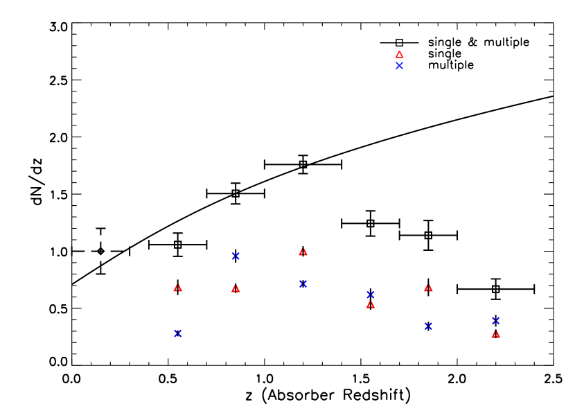
Figure 5: The redshift number density estimates from this survey for the various redshift bins. The $1.4<z<2.4$ redshift interval has been split into smaller bin size. The contributions from single and multiple cloud systems are also separately shown. The horizontal bars show the redshift bins for which the $dN/dz$ was calculated. The red triangles and the blue crosses are the $dN/dz$ values for the single and multiple clouds respectively. The $0<z<0.3$ data point is from a previous STIS/HST survey by Narayanan et al. (2005). The solid curve shows the expected number density for a non–evolving population of absorbers in a $\Lambda$CDM universe ($\Omega_{m}=0.3$ and $\Omega_{\Lambda}=0.7$) normalized at $z=0.9$ and $dN/dz=1.51$.The results distinctly suggest a peak in the number density of weak Mgii absorber at $z\sim 1.2$.

In figure 5, we focus on just the present VLT/UVES sample, and examine evolution of weak absorbers within the redshift interval $1.4<z<2.4$ more sequentially, with smaller redshift bins ($\Delta$z $\sim 0.3$). We can now see that not only is there a drop in the number density of weak Mgii absorbers at $z>1.4$, but it appears to be a steady drop. There is a distinct peak in $dN/dz$ in the bin centered at $z=1.2$.

Classifying the absorption systems in our sample as single cloud (a single kinematic component) and/or multiple cloud (with more than one kinematic components), we also calculated the redshift number densities of both classes separately for the various redshift bins. These are shown in also shown in figure 5. For consideration of this issue, even our larger sample is suffering from small number statistics. However, we see that both single-cloud and multiple-cloud weak Mgii absorbers do appear to exhibit a rise and then a fall in their number densities between $z=2.4$ and $z=0.4$.

3.3 Equivalent Width Distribution

The equivalent width distribution of Mgii systems is typically parameterized by fitting the data using either an exponential relationship of the form

$$\frac{\it{d}n(W)}{\it{d}W}=(N^{*}/W^{*})e^{-W/W^{*}}$$ (3)

where N^∗ and $W^{*}$ are best-fit parameters, or a power-law relationship of the form

$$\frac{\it{d}n(W)}{\it{d}W}=CW^{-\delta}$$ (4)

where C, a constant, and $\delta$, the power law index, are best-fit parameters.

3.4 Equivalent Width Distribution at $<z>=0.9$

Using a single power law, with $\delta=1.04$ and $C=0.54$, CRCV99 were able to produce an acceptable fit to the equivalent width distribution of both strong and weak systems, with the exception of the bin centered on the strongest absorbers at $W_{r}(2796)=2.2$ Å. The distribution indicated that, at $<z>=0.9$, there is a drastic increase in the number of systems toward the weak end of the distribution, with no indication of turn over in the power law distribution down to $W_{r}(2796)=0.02$ Å (see Fig. 6 of CRCV99).

Figure 6 shows the distribution function from results based on our survey for the redshift interval $0.4<z<1.4$ and for $W_{r}(2796)\geq 0.0165$ Å. The redshift interval and equivalent width lower limit were selected to be coincident with the values used by CRCV99. Since the equivalent width distribution is rapidly rising toward small values, it is critical to make comparisons in the same bins. For the three equivalent width bins at $W_{r}(2796)<0.3$ Å, the distribution for the bins centered at $0.15$ Å and $0.25$ Å are consistent with the results from CRCV99 survey, to within $\sim 1\sigma$. However, our measurement of $n(W_{r})$ for the lowest bin, at $0.06$ Å, is roughly a factor of two less than the CRCV99 result, a difference of $1.8\sigma$. Our measurement shows that there is a turn-over from the power law equivalent width distribution suggested in CRCV99, for $W_{r}(2796)<0.1$ Å. We considered the possibility that we are missing some of the weakest systems in our survey, but we think this is quite unlikely. Our survey is $78$ % complete at the lower equivalent width limit of $W_{r}(2796)=0.0165$ Å, whereas the CRCV99 survey, in comparison, is $70$ % complete at that same limit. We also note that if we use a limiting equivalent width of $0.02$ Å the discrepancy between the two survey results is at a negligible $1\sigma$ level. Thus we confirm that our results at $0.4<z<1.4$ are in agreement with CRCV99 in the sense that weak systems exceed strong systems in number by a factor of $\sim 3:1$.

More recently Nestor et al. (2005) presented results from a larger survey of strong Mgii absorption systems, identified in the spectra of $3700$ SDSS quasars. The equivalent width distribution of their sample ($0.3\leq W_{r}(2796)\leq 5.68$ Å) was fit using the exponential form described in equation (3), however the fit parameter, $W^{*}$ and the resultant normalization $N^{*}$, were $\sim 1\sigma$ lower than the parameters derived from the much smaller survey of Steidel & Sargent (1992). Figure 6 shows the fits from the various parameterizations for the equivalent width distributions of strong Mgii absorbers, with the more accurate results of Nestor et al. (2005) shown as the dashed curve. It is evident that an extrapolation of the exponential fit to the strong Mgii absorbers significantly underestimates the incidence of weak systems at $<z>=0.9$.

3.5 Equivalent Width Distribution at $<z>=1.9$

In figure 7, we present the equivalent width distribution for weak Mgii absorbers in the range $1.4<z<2.4$, and compare to that of the $0.4<z<1.4$ from our VLT/UVES sample. All low redshift datapoints are higher than the corresponding high redshift datapoints, due to the larger overall $dN/dz$ at $<z>=0.9$ than at $<z>=1.9$. The plot is log/linear in order to facilitate comparison to the equivalent width distribution of strong Mgii absorbers. Nestor et al. (2005) computed this distribution at redshift $1.311<z<2.269$, fitting it with the parameters $W^{*}=0.804$ and $N^{*}=1.267$. In Fig. 7, this function is given as a solid line. In fact, our datapoints for the $0.1$–$0.2$ Å and $0.2$–$0.3$ Å bins are consistent with an extrapolation of the equivalent width distribution for strong Mgii absorbers. Even the $0.0165$–$0.1$ Å bin is only a factor of two above the extrapolation. In contrast, Fig. 7 also shows that at $0.4<z<1.4$, there are significantly more weak Mgii absorbers (in all three equivalent width bins) than expected from an extrapolation of the strong Mgii absorber distribution function. The discrepancy is more than a factor of ten in the $0.0165$–$0.1$ Å bin.

4 Summary and Discussion

We have surveyed the VLT/UVES spectra of 81 quasars to search for weak Mgii absorbers over a redshift path $\Delta Z=77.3$, in the range $0.4<z<2.4$. Our survey is 86% complete at a rest-frame equivalent width limit $W_{r}(2796)=0.02$ Å. We confirm the result of LCT06 of a declining number density, $dN/dz$ of weak Mgii absorbers at $z>1.4$, finding a peak at $z\sim 1.2$ (see Figure 5). This general behavior is exhibited separately for the single and multiple-cloud weak Mgii absorbers. There may be differences in the evolution of these two classes, but they cannot be distinguished with a sample of the present size.

At $<z>=0.9$, the equivalent width distribution function for weak Mgii absorbers, shown in figure 7, rises substantially above an extrapolation of the exponential distribution that applies for strong Mgii absorbers (Nestor et al., 2005). However, at $<z>=1.9$, not only do we see a smaller number of weak Mgii absorbers relative to the expectations from evolution, in figure 7 we see only a slight excess over the extrapolation of the strong Mgii absorber distribution.

There may not be a very large separate weak Mgii absorbers population at $<z>=1.9$, and at higher redshifts. For example, if we were to extend a linear fit to the four highest redshift datapoints in figure 5, we would predict there would be no weak Mgii absorbers at $z>3$. Clearly, such an extrapolation is not realistic, since weak Mgii absorption is likely to have multiple causes at any redshift, however it highlights the fact that there really is a drastic evolution occurring.

LCT06 pointed out a rough coincidence between the peak period of incidence in weak Mgii absorbers (at $z\sim 1$) and the global star formation rate in the population of dwarf galaxies. More generally, it seems plausible that the evolution in $dN/dz$ of weak Mgii absorbers would relate to the rates of processes that give rise to this absorption. This remains feasible in view of the findings of our present survey. However, a variation of this type of scenario comes to mind based upon a recent study of the kinematics of strong Mgii absorbers by Mshar et al. (2006). In this new scenario it is not that the weak Mgii absorbers are not being generated at $z>2$. Instead, these structures would be evident, at high redshift, as parts of different types of absorbers, mostly as components of strong Mgii absorbers. The basis of this suggestion is this hypothesis that there is a three way connection between weak Mgii absorbers, satellite clouds of strong Mgii absorbers, and the extragalactic analogs of the Milky Way high velocity clouds (Mshar et al., 2006). At $z\sim 1$ many galaxies exist that are morphologically and kinematically similar to those in the present epoch (Charlton & Churchill, 1998). Typically, they have a dominant absorbing component as expected for a galaxy disk, with one or two weaker outlying components (i.e. satellite clouds) separated by $50$–$300$ km s^-1 from the main one. These satellite clouds look very similar to Milky Way high velocity clouds in their multiphase absorption properties (Fox et al., 2005; Collins et al., 2005; Fox et al., 2006). They also seem similar to single-cloud weak Mgii absorbers, which seem to have sheetlike or filamentary structures (Milutinović et al., 2006), perhaps like those of Milky Way Ovi high velocity clouds. Furthermore, if weak Mgii absorbers are predominantly found $30$–$100$ kpc from luminous galaxies, since they have a substantial cross–section relative to the galaxies themselves, it seems plausible that they are related to high velocity clouds.

Mshar et al. (2006) find an evolution in the kinematics of strong Mgii absorbers over the same redshift range that we are claiming evolution of the weak Mgii absorbers. The nature of the evolution is that the strong Mgii systems have a larger number of components at $z\sim 2$ than at $z\sim 1$, though their velocity spreads do not change. These extra components are very weak, but they act to fill in most of the velocity space spanning the full range of absorption. There are no longer separate and distinct “satellites”, nor is there evidence for single, well-formed galaxies. In fact, this seems quite analogous to the changes that take place in the visible morphologies of galaxies from $z\sim 2$ to $z\sim 1$. At the higher redshift galaxies typically have a clump-cluster (Elmegreen et al., 2005) or Tadpole-like morphology, with many separate star-forming regions. The kinematics of these systems are surely complex and it is likely that gas is spread through the region.

Finally, returning to the evolution of the weak Mgii absorbers that we have surveyed. We propose that the absence of them at $z\sim 2$ may be related to a lower probability of passing through just a single weak Mgii absorber. If the gas that produces Mgii absorption is really so irregularly distributed at $z\sim 2$ as suggested by the strong Mgii absorber kinematics, this seems plausible. It is a particularly appealing explanation if weak Mgii absorbers are the extragalactic high velocity clouds clustered among the protogalactic structures in a typical group. The structures that would produce single–cloud Mgii components and those that would produce multiple–cloud Mgii absorbers may be similar in this respect, in that both might tend to be kinematically connected at $z\sim 2$. It would be rare to observe an isolated single–cloud weak Mgii absorber because it would be kinematically connected to other Mgii absorbers. The same could apply for multiple–cloud weak Mgii absorbers if they are also produced by structures that tend to be concentrated around galaxies. At $z\sim 1$ these same types of structures form, not necessarily at an increased rate, but those that do form tend to be more separated from other absorbing structures for a longer period of time. This could produce the peak in the $dN/dz$ distribution of weak Mgii absorbers that we observe at $z\sim 1$. Subsequently, the processes that produce the structures that produce weak Mgii absorption (and perhaps high velocity clouds as well) may decline in order to give rise to the declining $dN/dz$ to the present.

Near–IR surveys of weak Mgii absorbers at $z>2.4$ will be needed to determine if the decline found up to this redshift continues up to higher values. Furthermore, detailed comparisons of the physical properties of weak Mgii absorbers and the satellite clouds surrounding strong Mgii absorbers. Finally, comparisons of the evolution of the ensemble of absorbers to the ensemble of gas distributions in high redshift groups, both from an observational and theoretical point of view, is ultimately needed.

This research was funded by NASA under grants NAG5-6399 and NNG04GE73G and by the National Science Foundation (NSF) under grant AST-04-07138. We also acknowledge the ESO archive facility for providing data.

Figure 1: The path length that was available in each quasar spectrum. The quasars are arranged from top to bottom and from left to right panel in increasing order of emission redshift (refer Table 1). The two vertical lines at $z=0.4$ and $z=2.4$ mark the limiting boundaries of our survey. We confined the lower redshift limit of our survey to $z=0.4$ since the coverage from our sample dropped significantly below that redshift.

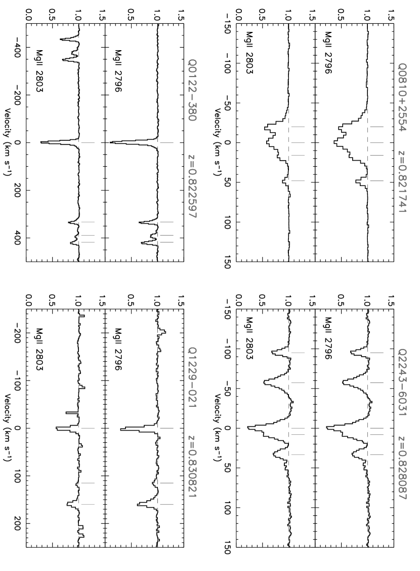
Figure 2a: Absorpiton profiles of the weak systems that were detected in our survey. The top panel in each plot shows the Mgii $\lambda 2796$ Å profile and the bottom panel the Mgii $\lambda 2803$ Å profile. The vertical tick marks represent the center of gaussian fits that were used to determine the equivalent width of the absorbption system. Figures 2a-2e show only a few examples of the weak Mgii systems that we identified in our survey. The absorption profile of all systems identified in our survey will be published in the online version of the journal

.

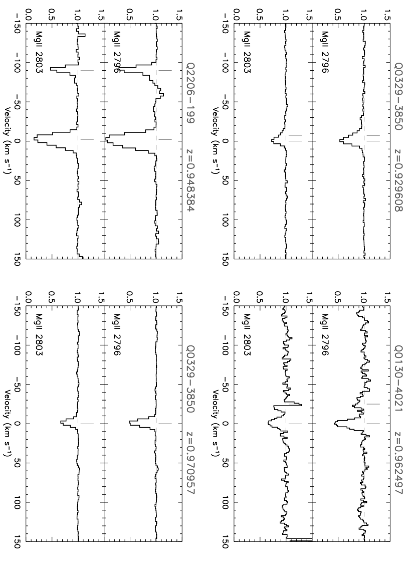
Figure 2b: Contd. Figure 2a

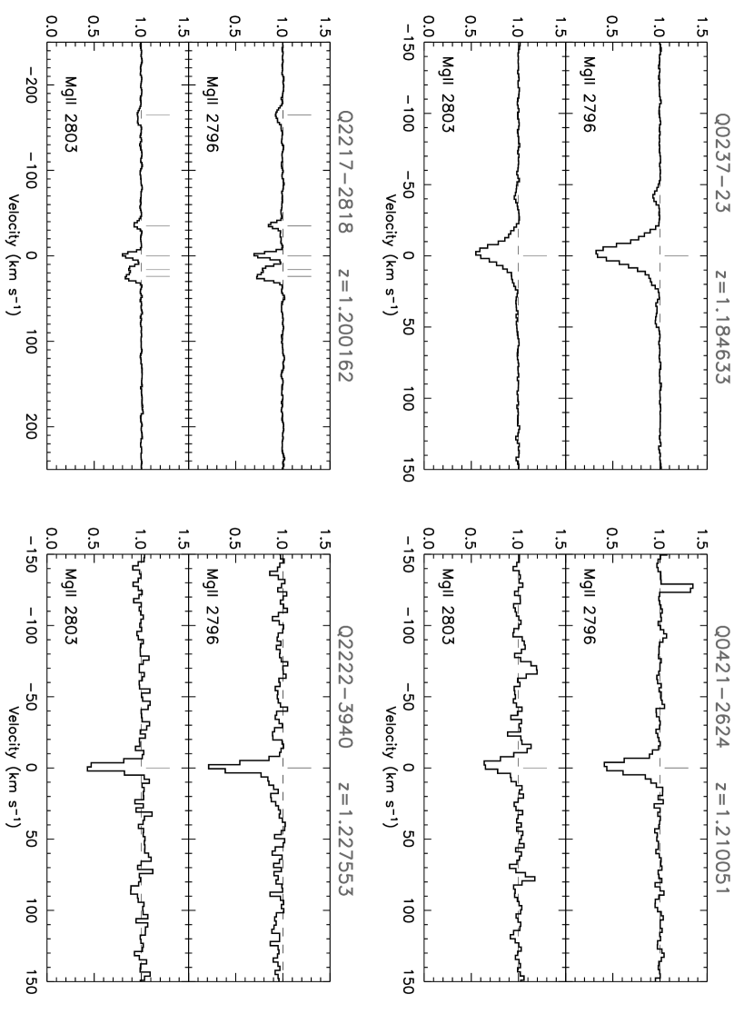
Figure 2c: Contd. Figure 2a

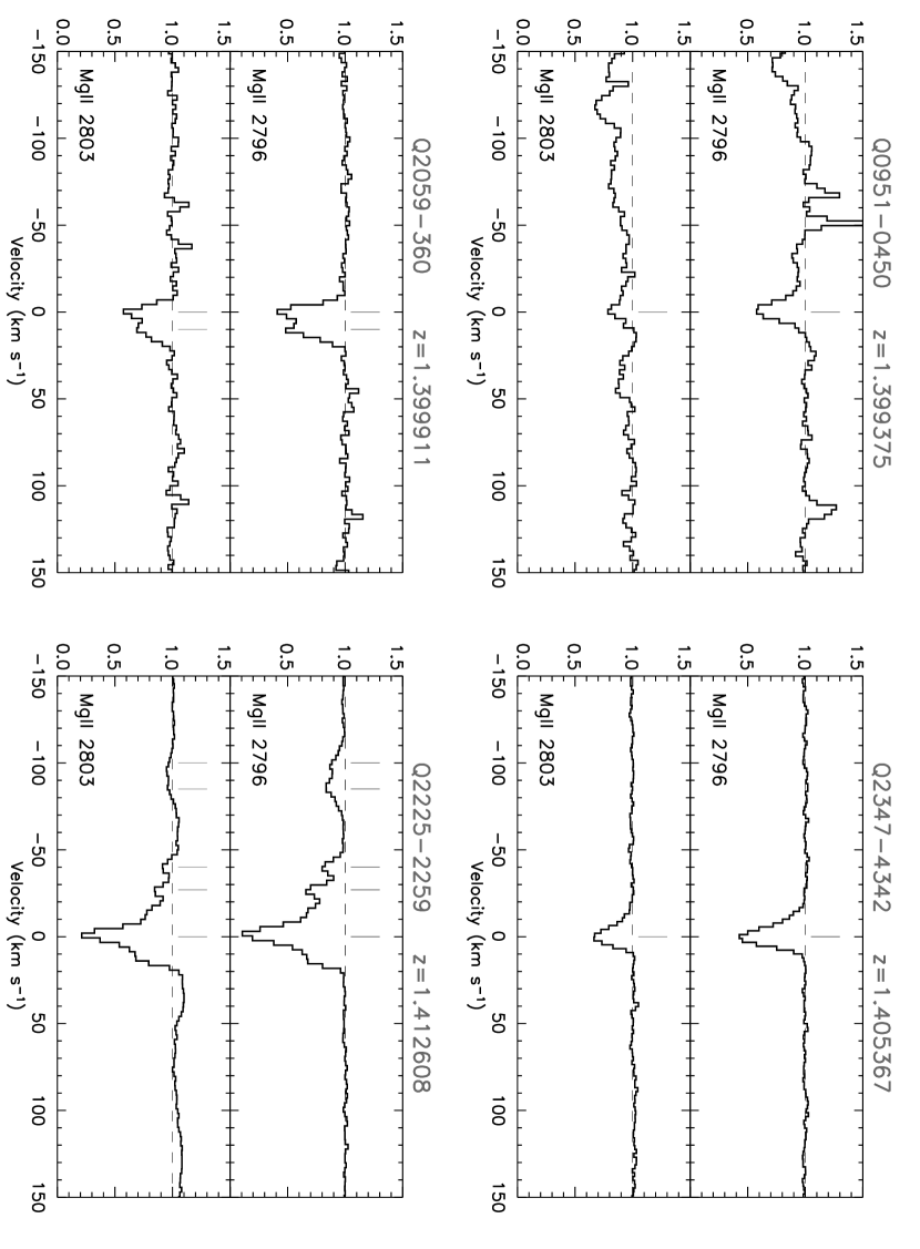
Figure 2d: Contd. Figure 2a

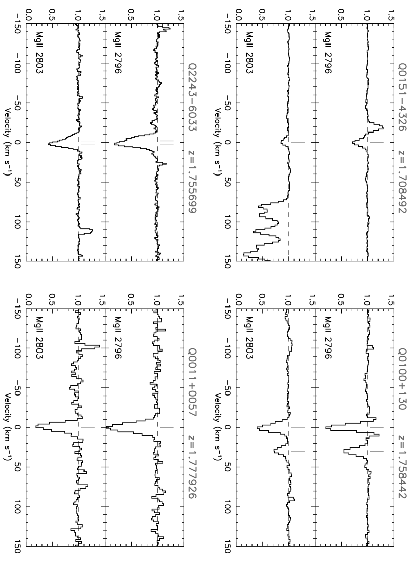
Figure 2e: Contd. Figure 2a

Figure 3: The completeness of the survey is depicted in this figure by plotting the cumulative redshift path as a fucntion of the rest–frame equivalent width, $W_{r}(2796)$, for the redshift interval $0.4<z<2.4$.

Figure 4: The redshift number density estimates from this survey for the various redshift bins (see Table 3). Also included are the $dN/dz$ constrains from the previous three surveys. Narayanan et al. (2005) was a survey for weak Mgii systems in the present day universe ($0<z<0.3$). The CRCV99 survey covered the redshift window $0.4<z<1.4$, and the LCT06 survey covered the same redshift range as this survey ($0.4<z<2.4$). The solid curve represents no–evolution expectation in a $\Lambda$CDM universe ($\Omega_{m}=0.3$ and $\Omega_{\Lambda}=0.7$) normalized at $z=0.9$ and $dN/dz=1.74$, the normalization used by CRCV99. Systems with $W_{r}<0.02$ Å are excluded from our $dN/dz$ estimate, in order to correspond with the equivalent width limits chosen by the CRCV99 and LCT06 surveys.

Figure 6: The equivalent width distribution for strong and weak systems inside the redshift interval $0.4<z<1.4$. The three equivalent width bins are [0.0165, 0.1], [0.1, 0.2] and [0.2, 0.3] Å respectively. The bins were selected to match with the CRCV99 choice of bins. The horizontal bars on each data point represents the equivalent width bins in units of Angstroms. The vertical bars are the error bars for each $n(W_{r})$. The points marked with asterisk are results from our survey. The points marked with triangle are from the Keck/HIRES weak Mgii survey by CRCV99. The square points represent strong systems from Steidel & Sargent (1992). The solid sloped line indicates the power-law function given by equation (4) and based on best-fit parameters derived by CRCV99. The dashed-dot curve indicates the exponential function given by equation (3) and based on best-fit parameters derived by SS92 from fitting strong systems. The dashed curve also represents the exponential function, but with best-fit parameters presented by Nestor et al. (2005) from their survey of strong systems using the SDSS data. The thin vertical solid line marks the boundary between weak and strong absorbers. Our survey is $78$ % complete at the lowest equivalent width limit of $W_{r}=0.0165$ Å in comparision to CRCV99 which is $70$ % complete at that same limit.

Figure 7: The equivalent width distribution of weak systems within the redshift interval $1.4<z<2.4$ from our survey. The horizontal bars represent individual equivalent width bins in Angstroms. The veritcal bars are error bars associated with each $n(W_{r})$. The three slanting lines represent the exponential form of equivalent width distribution as described in equation (3) for different redshift intervals with best fit-parameters taken from Nestor et al. (2005). The solid line with best-fit parameters of $W^{*}=0.702$ and $N^{*}=1.187$ defines the exponential distribution inside the interval $1.311<z<2.269$. The dashed line with best-fit parameters of $W^{*}=0.741$ and $N^{*}=1.171$ describes the exponential distribution inside the interval $0.871<z<1.311$. The dash-dot-dot line with best-fit parameters of $W^{*}=0.585$ and $N^{*}=1.216$ is for the redshift interval $0.366<z<0.871$. For the sake of comparision, the distribution function $n(W_{r})$ for the lower redshift interval $0.4<z<1.4$ is also plotted.

Table 1: UVES/VLT ARCHIVE QSO DATA SET

Target	zQSO	V	${\lambda}$ Å	Setting	texp(s)	Prog.ID	PI
TON1480	$0.614$	$17$	$3530-6650$	$390{\times}564$	$18470$	69.A-0371	Savaglio
Q0300+0048	$0.89$	$19.4(g)$	$3070-10000$	$437{\times}860$	$4500$	267.B-5698	Hutsemekers
				$346{\times}580$	$4500$	267.B-5698	Hutsemekers
3c336	$0.927$	$17.5$	$3530-6650$	$390{\times}564$	$9800$	69.A-0371	Savaglio
Q0827+243	$0.939$	$17.3$	$3050-6650$	$346{\times}564$	$14400$	68.A-0170	Mallen-Ornelas
				$346{\times}564$	$19670$	69.A-0371	Savaglio
Q1229-021	$1.038$		$3530-6650$	$390{\times}564$	$10800$	68.A-0170	Mallen-Ornelas
Q1127-14	$1.187$		$3050-6800$	$346{\times}580$	$15300$	67.A-0567	Lane
				$390{\times}564$	$9600$	69.A-0371	Savaglio
Q1243-072	$1.286$	$18.0$	$3050-6800$	$346{\times}580$	$12000$	69.A-0410	Athreya
Q1453+0029	$1.297$	$21.6(g)$	$4940-10000$	$580$	$9000$	267.B-5698	Hutsemekers
				$860$	$9000$	267.B-5698	Hutsemekers
Q0952+179	$1.472$	$17.2$	$3050-6650$	$346{\times}564$	$17100$	69.A-0371	Savaglio
Q2215-0045	$1.475$		$3060-9950$	$437{\times}860$	$10800$	267.B-5698	Hutsemekers
				$346{\times}580$	$10800$	267.B-5698	Hutsemekers
Q0810+2554	$1.5$	$15.4$	$3050-6640$	$346{\times}564$	$48900$	68.A-0107	Reimers
Q0926-0201	$1.661$	$16.4$	$3060-10000$	$437{\times}860$	$3065$	72.A-0446	Murphy
				$346{\times}580$	$12260$	72.A-0446	Murphy
Q1629+120	$1.795$		$3050-6800$	$346{\times}580$	$12000$	69.A-0410	Athreya
Q0141-3932	$1.807$		$3060-10000$	$437{\times}860$	$14400$	67.A-0280	Lopez
				$346{\times}580$	$25200$	67.A-0280(A)	Lopez
Q0328-272	$1.816$		$3500-6630$	$390{\times}564$	$13200$	072.B-0218	Baker
Q2225-2258	$1.891$	$17.6$	$3050-10000$	$346{\times}580$	$28800$	67.A-0280	Lopez
				$437{\times}860$	$14400$	67.A-0280	Lopez
Q0136-231	$1.893$	$18.8$	$3500-6640$	$390{\times}564$	$9000$	072.B-0218	Baker
				$520$	$3600$	072.B-0218	Baker
Q0128-2150	$1.900$	$15.6$	$3050-6800$	$346{\times}580$	$6130$	72.A-0446	Murphy
Q2044-168	$1.932$	$17.36$	$3520-9900$	$410{\times}800$	$6600$	71.B-0106	Pettini
Q0429-4901	$1.940$	$16.2$	$3050-10080$	$437{\times}860$	$18835$	66.A-0221	Lopez
				$346{\times}580$	$10800$	66.A-0221	Lopez
Q0105+061	$1.96$	$17.2$	$3516-9860$	$410{\times}800$	$9900$	71.B-0106	Pettini
Q1157+014	$1.9997$	$17.0$	$3520-7400$	$380{\times}580$	$3600$	67.A-0078	Ledoux
				$380{\times}750$	$7200$	67.A-0078	Ledoux
				$390{\times}580$	$1800$	68.A-0461	Kanekar
Q1331+170	$2.084$		$3050-10000$	$346{\times}860$	$13500$	67.A-0022	D’Odorico
Q0013-0029	$2.087$	$17$	$3060-9890$	$437{\times}750$	$10800$	66.A-0624	Ledoux
				$346{\times}580$	$19800$	66.A-0624	Ledoux
				$346{\times}564$	$54000$	267.A-5714	Petitjean
				$564$	$10800$	267.A-5714	Petitjean
Q1246-0217	$2.106$	$18.1$	$3525-6650$	$390{\times}564$	$5400$	67.A-0146	Vladilo
Q1341-1020	$2.135$	$17.1$	$3060-10400$	$346{\times}580$	$32400$	160.A-0106	Bergeron
Q0010-0012	$2.145$	$19.43$	$3050-6650$	$346{\times}564$	$5400$	68.A-0600	Ledoux
Q2222-3939	$2.18$	$17.9$	$3530-6640$	$390{\times}564$	$1800$	072.A-0442	Lopez
Q0122-380	$2.200$	$17.1$	$3060-10190$	$346{\times}580$	$21600$	160.A-0106	Bergeron
Q1444+014	$2.206$		$3520-5830$	$390{\times}564$	$18000$	65.O-0158	Pettini
				$380{\times}564$	$10800$	67.A-0078	Ledoux
				$390{\times}564$	$10800$	69.B-0108	Srianand
				$390{\times}564$	$14400$	71.B-0136	Srianand
Q1448-232	$2.215$	$17$	$3060-10070$	$346{\times}580$	$28800$	160.A-0106	Bergeron
				$437{\times}860$	$21600$	160.A-0106	Bergeron
Q0237-23	$2.223$	$16.8$	$3060-10070$	$346{\times}580$	$21600$	160.A-0106	Bergeron
				$437{\times}860$	$21600$	160.A-0106	Bergeron
Q0549-213	$2.245$	$20$	$3500-6640$	$390{\times}564$	$12000$	072.B-0218	Baker
Q0425-5214	$2.25$	$17.8$	$3520-6645$	$390{\times}564$	$1800$	072.A-0442	Lopez
Q0049-2820	$2.256$	$18.42$	$3520-6645$	$390{\times}580$	$1800$	072.A-0442	Lopez
Q0421-2624	$2.277$	$18.08$	$3520-6640$	$390{\times}564$	$1800$	072.A-0442	Lopez
Q0001-2340	$2.28$	$16.7$	$3060-10070$	$346{\times}580$	$21600$	160.A-0106	Bergeron
				$437{\times}860$	$21600$	160.A-0106	Bergeron
Q1114-220	$2.282$	$20.2$	$3540-6645$	$390{\times}564$	$14120$	71.B-0081	Baker
Q0011+0055	$2.31$	$19.1(g)$	$3770-10000$	$437{\times}860$	$7200$	267.B-5698	Hutsemekers
Q0551-3637	$2.318$	$17.0$	$3060-9370$	$437{\times}750$	$8100$	66.A-0624	Ledoux
				$346{\times}580$	$18000$	66.A-0624	Ledoux
Q2116-358	$2.341$	$17$	$3530-6640$	$390{\times}564$	$7200$	65.O-0158	Pettini
Q0042-2930	$2.388$	$17.81$	$3530-6800$	$390{\times}580$	$1800$	072.A-0442	Lopez
Q0109-3518	$2.405$	$16.6$	$3060-10070$	$346{\times}580$	$25200$	160.A-0106	Bergeron
				$437{\times}860$	$21600$	160.A-0106	Bergeron
Q1122-1648	$2.405$	$17.7$	$3060-10070$	$346{\times}580$	$26400$	Sci. Veri
				$437{\times}860$	$27000$	Sci. Veri
Q2217-2818	$2.406$	$16.0$	$3060-9890$	$346{\times}580$	$16200$	Comm.
				$390{\times}564$	$10800$	Comm.
Q2132-433	$2.420$	$18.18$	$3500-6640$	$390{\times}564$	$3600$	65.O-0158	Pettini
Q0329-385	$2.435$	$17.2$	$3070-8500$	$346{\times}580$	$21600$	160.A-0106	Bergeron
				$437{\times}860$	$21600$	160.A-0106	Bergeron
Q2314-409	$2.448$	$17.9$	$3520-6640$	$390{\times}564$	$13680$	267.A-5707	Ellison
Q1158-1843	$2.448$	$16.9$	$3070-10070$	$346{\times}580$	$21600$	160.A-0106	Bergeron
				$437{\times}860$	$21600$	160.A-0106	Bergeron
Q2206-199	$2.56$	$17.3$	$3420-6640$	$390{\times}564$	$17100$	65.O-0158	Pettini
Q1140+2711	$2.630$	$17.0$	$3775-10000$	$437{\times}860$	$45400$	69.A-0246	Reimers
Q0453-423	$2.657$	$17.3$		$346{\times}580$	$28800$	160.A-0106	Bergeron
				$437{\times}860$	$28800$	160.A-0106	Bergeron
Q0100+1300	$2.681$	$16.57$	$3520-10000$	$390{\times}860$	$7200$	67.A-0022	D’Odorico
Q0329-255	$2.685$	$17.51$	$3060-10070$	$346{\times}580$	$46800$	160.A-0106	Bergeron
				$437{\times}860$	$39600$	160.A-0106	Bergeron
Q0151-4326	$2.74$	$17.19$	$3060-10070$	$346{\times}580$	$28800$	160.A-0106	Bergeron
				$437{\times}860$	$32400$	160.A-0106	Bergeron
Q0002-422	$2.76$	$17.2$	$3160-10070$	$346{\times}580$	$28800$	160.A-0106	Bergeron
				$437{\times}860$	$39600$	160.A-0106	Bergeron
Q1151+068	$2.762$	$18.6$	$3705-10000$	$346{\times}580$	$10800$	65.O-0158	Pettini
				$437{\times}860$	$10800$	65.O-0158	Pettini
Q0112+0300	$2.81$		$3540-6800$	$390{\times}580$	$3600$	66.A-0624	Ledoux
Q2347-4342	$2.88$	$16.3$	$3100-10070$	$346{\times}580$	$21600$	160.A-0106	Bergeron
				$437{\times}860$	$28800$	160.A-0106	Bergeron
Q1337+113	$2.919$	$18.7$	$3540-9380$	$410{\times}750$	$10800$	67.A-0078	Ledoux
Q2243-6031	$3.01$	$18.3$	$3140-10000$	$346{\times}580$	$14400$	65.O-0411	Lopez
				$437{\times}860$	$11400$	65.O-0411	Lopez
Q0130-4021	$3.023$	$17.02$	$3550-6800$	$390{\times}580$	$3065$	70.B-0522	Bomans
Q0102-1902	$3.04$		$3620-10000$	$390{\times}564$	$3600$	67.A-0146	Vladilo
				$437{\times}860$	$10800$	67.A-0146	Vladilo
Q0940-1050	$3.083$	$16.6$	$3110-10070$	$346{\times}580$	$18000$	160.A-0106	Bergeron
				$437{\times}860$	$14400$	160.A-0106	Bergeron
Q2059-360	$3.092$	$18.62$	$3750-9280$	$433{\times}740$	$18000$	67.A-0078	Ledoux
Q0058-2914	$3.093$	$18.7$	$3550-10000$	$390{\times}580$	$5400$	66.A-0624	Ledoux
				$437{\times}860$	$34200$	67.A-0146	Vladilo
Q0420-388	$3.117$	$16.9$	$3760-10070$	$390{\times}564$	$28800$	160.A-0106	Bergeron
				$437{\times}860$	$28800$	160.A-0106	Bergeron
Q2204-408	$3.155$	$17.57$	$3520-6800$	$390{\times}580$	$6600$	71.B-0106	Pettini
				$580$	$9900$	71.B-0106	Pettini
Q2126-158	$3.28$	$17.3$	$3520-9600$	$390{\times}564$	$32400$	160.A-0106	Bergeron
				$437{\times}860$	$28800$	160.A-0106	Bergeron
Q1209+0919	$3.3$	$18.5$	$3520-7770$	$390{\times}564$	$5400$	67.A-0146	Vladilo
				$437{\times}860$	$14765$	67.A-0146	Vladilo
				$390{\times}580$	$3600$	73.B-0787	Dessauges-Zavadsky
CTQ0298	$3.37$	$17.60$	$3520-8550$	$390{\times}564$	$10800$	68.A-0492	D’Odorico
				$436{\times}800$	$14400$	68.A-0492	D’Odorico
Q0055-269	$3.66$	$17.47$	$3060-7505$	$346{\times}580$	$17000$	65.O-0296	D’Odorico
				$437{\times}800$	$16300$	65.O-0296	D’Odorico
				$346{\times}565$	$9300$	65.O-0296	D’Odorico
				$565$	$8800$	65.O-0296	D’Odorico
Q1418-064	$3.689$	$18.5$	$3765-9945$	$437{\times}860$	$3575$	69.A-0051	Pettini
				$437{\times}860$	$3814$	71.A-0539	Kanekar
				$437{\times}860$	$7150$	71.A-0067	Ellison
Q1621-0042	$3.7$		$3530-6800$	$390{\times}580$	$28105$	075.A-0464	Kim
Q2000-330	$3.773$	$17.3$	$3495-9945$	$580$	$3600$	65.O-0299	D’Odorico
				$390{\times}560$	$32400$	166.A-0106	Bergeron
				$437{\times}860$	$32400$	166.A-0106	Bergeron
Q1108-0747	$3.922$	$18.10$	$3765-9945$	$520$	$4500$	67.A-0022	D’Odorico
				$520$	$6000$	68.A-0492	D’Odorico
				$480{\times}800$	$7200$	68.A-0492	D’Odorico
				$437$	$3598$	68.B-0115	Molaro
				$580$	$4800$	68.B-0115	Molaro
				$437{\times}860$	$9600$	68.B-0115	Molaro
Q0401-1711	$4.23$	$18.7$	$4785-9880$	$580$	$6000$	074.A-0306	D’Odorico
				$860$	$6625$	074.A-0306	D’Odorico
				$800$	$2617$	71.B-0106	Pettini
Q2344+0342	$4.239$	$18.6$	$4635-9890$	$800$	$9000$	65.O-0296	D’Odorico
				$565$	$4500$	65.O-0296	D’Odorico
Q0951-0450	$4.369$	$18.9$	$4785-6805$	$580$	$30960$	072.A-0558	Vladilo
Q1114-0822	$4.495$	$19.4$	$4785-10000$	$580{\times}860$	$14415$	074.A-0801	Molaro
Q1202-0725	$4.694$	$17.5$	$3535-10000$	$437{\times}860$	$10958$	66.A-0594	Molaro
				$390{\times}580$	$38693$	66.A-0594	Molaro
				$580$	$18000$	166.A-0106	Bergeron
				$860$	$7200$	166.A-0106	Bergeron
				$860$	$17000$	71.B-0106	Pettini

Note. — This table provides details of the archived VLT/UVES spectra that were used in our survey. The second and third column lists the redshift of the quasar and its magnitude as given by Simbad and/or NED data base. The fourth column gives the wavelength coverage for each case. The fifth column is the cross-disperser settings that were used for the various exposures. The sixth column gives the total exposure time (in seconds). The program ID and the PI of the program are listed in the final two columns.

Table 2: WEAK Mgii SYSTEMS DETECTED

QSO	zabs	W${}_{r}(2796)$	W${}_{r}(2803)$	DR	Z($W_{r}$,DR)
Q1127-145	$0.190587$	$0.137~{}{\pm}~{}0.009$	$0.054~{}{\pm}~{}0.007$	$2.54~{}{\pm}~{}0.37$	$-$
Q0827+243	$0.259000$	$0.273~{}{\pm}~{}0.006$	$0.201~{}{\pm}~{}0.005$	$1.36~{}{\pm}~{}0.05$	$-$
Q1127-145	$0.328258$	$0.028~{}{\pm}~{}0.004$	$0.018~{}{\pm}~{}0.000$	$1.56~{}{\pm}~{}0.22$	$-$
Q0141-3932	$0.340005$	$0.227~{}{\pm}~{}0.003$	$0.116~{}{\pm}~{}0.003$	$1.96~{}{\pm}~{}0.06$	$-$
Q1444+014	$0.444019$	$0.228~{}{\pm}~{}0.003$	$0.113~{}{\pm}~{}0.003$	$2.02~{}{\pm}~{}0.06$	77.66
Q0001-2340	$0.452414$	$0.105~{}{\pm}~{}0.001$	$0.071~{}{\pm}~{}0.001$	$1.48~{}{\pm}~{}0.03$	77.33
Q0011+0055	$0.487243$	$0.244~{}{\pm}~{}0.019$	$0.129~{}{\pm}~{}0.016$	$1.89~{}{\pm}~{}0.28$	77.70
Q0551-3637	$0.505268$	$0.083~{}{\pm}~{}0.007$	$0.062~{}{\pm}~{}0.022$	$1.34~{}{\pm}~{}0.49$	77.15
Q1158-1843	$0.506041$	$0.022~{}{\pm}~{}0.001$	$0.013~{}{\pm}~{}0.001$	$1.69~{}{\pm}~{}0.15$	68.48
Q1444+014	$0.509653$	$0.140~{}{\pm}~{}0.005$	$0.083~{}{\pm}~{}0.005$	$1.69~{}{\pm}~{}0.12$	77.41
Q2116-358	$0.539154$	$0.102~{}{\pm}~{}0.013$	$0.084~{}{\pm}~{}0.004$	$1.21~{}{\pm}~{}0.17$	77.35
Q0328-272	$0.570827$	$0.168~{}{\pm}~{}0.008$	$0.098~{}{\pm}~{}0.007$	$1.71~{}{\pm}~{}0.15$	77.56
Q0429-4901	$0.584249$	$0.017~{}{\pm}~{}0.002$	$0.008~{}{\pm}~{}0.001$	$2.13~{}{\pm}~{}0.36$	59.34
Q2217-2818	$0.599512$	$0.114~{}{\pm}~{}0.001$	$0.067~{}{\pm}~{}0.003$	$1.70~{}{\pm}~{}0.08$	77.34
Q0013-0029	$0.635069$	$0.162~{}{\pm}~{}0.022$	$0.091~{}{\pm}~{}0.009$	$1.78~{}{\pm}~{}0.30$	77.5
Q0001-2340	$0.685957$	$0.033~{}{\pm}~{}0.001$	$0.018~{}{\pm}~{}0.001$	$1.83~{}{\pm}~{}0.12$	74.19
Q1229-021	$0.700377$	$0.010~{}{\pm}~{}0.001$	$0.008~{}{\pm}~{}0.002$	$1.25~{}{\pm}~{}0.34$	46.52
3c336	$0.702901$	$0.028~{}{\pm}~{}0.004$	$0.022~{}{\pm}~{}0.003$	$1.27~{}{\pm}~{}0.25$	72.94
Q0151-4326	$0.737248$	$0.022~{}{\pm}~{}0.001$	$0.019~{}{\pm}~{}0.001$	$1.16~{}{\pm}~{}0.08$	68.71
Q1229-021	$0.756921$	$0.298~{}{\pm}~{}0.004$	$0.238~{}{\pm}~{}0.004$	$1.25~{}{\pm}~{}0.03$	77.82
Q1229-021	$0.768862$	$0.026~{}{\pm}~{}0.002$	$0.011~{}{\pm}~{}0.001$	$2.36~{}{\pm}~{}0.28$	68.28
Q0109-3518	$0.769646$	$0.033~{}{\pm}~{}0.001$	$0.018~{}{\pm}~{}0.001$	$1.83~{}{\pm}~{}0.12$	74.19
Q2116-358	$0.775270$	$0.238~{}{\pm}~{}0.039$	$0.110~{}{\pm}~{}0.014$	$2.16~{}{\pm}~{}0.45$	77.66
Q2217-2818	$0.786572$	$0.207~{}{\pm}~{}0.003$	$0.114~{}{\pm}~{}0.001$	$1.82~{}{\pm}~{}0.03$	77.62
Q2132-433	$0.793570$	$0.184~{}{\pm}~{}0.008$	$0.118~{}{\pm}~{}0.008$	$1.56~{}{\pm}~{}0.13$	77.61
Q0042-2930	$0.798665$	$0.243~{}{\pm}~{}0.008$	$0.149~{}{\pm}~{}0.006$	$1.64~{}{\pm}~{}0.09$	77.71
Q1122-1648	$0.806215$	$0.245~{}{\pm}~{}0.001$	$0.154~{}{\pm}~{}0.001$	$1.59~{}{\pm}~{}0.01$	77.72
Q1158-1843	$0.818146$	$0.063~{}{\pm}~{}0.001$	$0.038~{}{\pm}~{}0.001$	$1.66~{}{\pm}~{}0.05$	76.67
Q0810+2554	$0.821741$	$0.252~{}{\pm}~{}0.002$	$0.166~{}{\pm}~{}0.002$	$1.52~{}{\pm}~{}0.02$	77.76
Q0122-380	$0.822597$	$0.253~{}{\pm}~{}0.007$	$0.138~{}{\pm}~{}0.012$	$1.83~{}{\pm}~{}0.17$	77.73
Q2243-6031	$0.828087$	$0.242~{}{\pm}~{}0.003$	$0.135~{}{\pm}~{}0.004$	$1.79~{}{\pm}~{}0.06$	77.70
Q1229-021	$0.830821$	$0.126~{}{\pm}~{}0.004$	$0.071~{}{\pm}~{}0.003$	$1.77~{}{\pm}~{}0.09$	77.34
Q2225-2258	$0.831374$	$0.031~{}{\pm}~{}0.002$	$0.020~{}{\pm}~{}0.002$	$1.55~{}{\pm}~{}0.18$	73.80
Q0810+2554	$0.831727$	$0.171~{}{\pm}~{}0.002$	$0.084~{}{\pm}~{}0.002$	$2.04~{}{\pm}~{}0.05$	77.5
Q2314-409	$0.843114$	$0.044~{}{\pm}~{}0.003$	$0.028~{}{\pm}~{}0.004$	$1.57~{}{\pm}~{}0.25$	75.81
Q0013-0029	$0.857469$	$0.142~{}{\pm}~{}0.004$	$0.123~{}{\pm}~{}0.004$	$1.15~{}{\pm}~{}0.05$	77.45
Q0453-4230	$0.895865$	$0.034~{}{\pm}~{}0.001$	$0.019~{}{\pm}~{}0.001$	$1.79~{}{\pm}~{}0.11$	74.45
Q0109-3518	$0.895295$	$0.020~{}{\pm}~{}0.001$	$0.011~{}{\pm}~{}0.001$	$1.82~{}{\pm}~{}0.19$	65.54
Q0122-380	$0.910146$	$0.061~{}{\pm}~{}0.004$	$0.028~{}{\pm}~{}0.011$	$2.18~{}{\pm}~{}0.87$	76.42
Q0102-1902	$0.916743$	$0.294~{}{\pm}~{}0.010$	$0.228~{}{\pm}~{}0.012$	$1.30~{}{\pm}~{}0.08$	77.82
Q03290-3850	$0.929608$	$0.072~{}{\pm}~{}0.007$	$0.037~{}{\pm}~{}0.004$	$1.95~{}{\pm}~{}0.28$	76.73
Q2206-199	$0.948384$	$0.255~{}{\pm}~{}0.002$	$0.180~{}{\pm}~{}0.002$	$1.42~{}{\pm}~{}0.02$	77.77
Q0130-4021	$0.962497$	$0.089~{}{\pm}~{}0.004$	$0.060~{}{\pm}~{}0.004$	$1.48~{}{\pm}~{}0.13$	77.19
Q0329-3850	$0.970957$	$0.051~{}{\pm}~{}0.001$	$0.031~{}{\pm}~{}0.002$	$1.65~{}{\pm}~{}0.11$	76.23
Q0329-2550	$0.992631$	$0.283~{}{\pm}~{}0.011$	$0.167~{}{\pm}~{}0.006$	$1.69~{}{\pm}~{}0.09$	77.8
Q1448-232	$1.019089$	$0.033~{}{\pm}~{}0.005$	$0.015~{}{\pm}~{}0.002$	$2.20~{}{\pm}~{}0.44$	73.37
Q0453-4230	$1.039514$	$0.189~{}{\pm}~{}0.003$	$0.096~{}{\pm}~{}0.001$	$1.97~{}{\pm}~{}0.04$	77.61
Q2217-2818	$1.054310$	$0.046~{}{\pm}~{}0.002$	$0.024~{}{\pm}~{}0.001$	$1.92~{}{\pm}~{}0.12$	75.88
Q2217-2818	$1.082920$	$0.125~{}{\pm}~{}0.001$	$0.064~{}{\pm}~{}0.001$	$1.95~{}{\pm}~{}0.03$	77.34
Q0042-2930	$1.091866$	$0.162~{}{\pm}~{}0.005$	$0.136~{}{\pm}~{}0.004$	$1.19~{}{\pm}~{}0.05$	77.53
Q0926-0201	$1.096336$	$0.020~{}{\pm}~{}0.001$	$0.015~{}{\pm}~{}0.001$	$1.33~{}{\pm}~{}0.11$	66.11
Q2222-3939	$1.098126$	$0.184~{}{\pm}~{}0.015$	$0.136~{}{\pm}~{}0.015$	$1.35~{}{\pm}~{}0.19$	77.61
Q1444+014	$1.102026$	$0.142~{}{\pm}~{}0.001$	$0.181~{}{\pm}~{}0.001$	$0.78~{}{\pm}~{}0.01$	77.47
Q2347-4342	$1.109640$	$0.040~{}{\pm}~{}0.004$	$0.028~{}{\pm}~{}0.003$	$1.43~{}{\pm}~{}0.21$	75.51
Q1444+014	$1.129162$	$0.244~{}{\pm}~{}0.006$	$0.151~{}{\pm}~{}0.007$	$1.62~{}{\pm}~{}0.08$	77.72
Q0013-0029	$1.146810$	$0.047~{}{\pm}~{}0.001$	$0.019~{}{\pm}~{}0.001$	$2.47~{}{\pm}~{}0.14$	75.33
Q1151+068	$1.153727$	$0.108~{}{\pm}~{}0.003$	$0.077~{}{\pm}~{}0.003$	$1.40~{}{\pm}~{}0.07$	77.35
CTQ0298	$1.160456$	$0.049~{}{\pm}~{}0.003$	$0.033~{}{\pm}~{}0.003$	$1.48~{}{\pm}~{}0.16$	76.16
Q1621-0042	$1.174581$	$0.237~{}{\pm}~{}0.012$	$0.115~{}{\pm}~{}0.025$	$2.06~{}{\pm}~{}0.45$	77.66
Q0109-3518	$1.182684$	$0.135~{}{\pm}~{}0.001$	$0.098~{}{\pm}~{}0.001$	$1.38~{}{\pm}~{}0.02$	77.42
Q0237-23	$1.184633$	$0.140~{}{\pm}~{}0.005$	$0.083~{}{\pm}~{}0.004$	$1.69~{}{\pm}~{}0.10$	77.41
Q2217-2818	$1.200162$	$0.099~{}{\pm}~{}0.002$	$0.043~{}{\pm}~{}0.001$	$2.30~{}{\pm}~{}0.07$	77.24
Q0421-2624	$1.210051$	$0.065~{}{\pm}~{}0.002$	$0.032~{}{\pm}~{}0.002$	$2.03~{}{\pm}~{}0.14$	76.60
Q2222-3939	$1.227553$	$0.114~{}{\pm}~{}0.005$	$0.042~{}{\pm}~{}0.003$	$2.71~{}{\pm}~{}0.23$	77.14
Q0926-0201	$1.232203$	$0.069~{}{\pm}~{}0.004$	$0.032~{}{\pm}~{}0.003$	$2.16~{}{\pm}~{}0.24$	76.64
Q1122-1648	$1.234160$	$0.200~{}{\pm}~{}0.000$	$0.130~{}{\pm}~{}0.002$	$1.54~{}{\pm}~{}0.02$	77.63
Q2059-360	$1.242973$	$0.015~{}{\pm}~{}0.001$	$0.010~{}{\pm}~{}0.002$	$1.50~{}{\pm}~{}0.32$	58.21
Q2000-330	$1.249864$	$0.032~{}{\pm}~{}0.001$	$0.022~{}{\pm}~{}0.001$	$1.45~{}{\pm}~{}0.08$	74.13
CTQ0298	$1.256069$	$0.057~{}{\pm}~{}0.004$	$0.068~{}{\pm}~{}0.002$	$0.84~{}{\pm}~{}0.06$	76.64
Q0136-231	$1.261761$	$0.102~{}{\pm}~{}0.003$	$0.071~{}{\pm}~{}0.005$	$1.44~{}{\pm}~{}0.11$	77.33
Q1209+0919	$1.264983$	$0.083~{}{\pm}~{}0.007$	$0.061~{}{\pm}~{}0.007$	$1.35~{}{\pm}~{}0.19$	77.14
Q0328-272	$1.269054$	$0.047~{}{\pm}~{}0.011$	$0.043~{}{\pm}~{}0.085$	$1.09~{}{\pm}~{}2.17$	76.13
Q0136-231	$1.285796$	$0.021~{}{\pm}~{}0.003$	$0.015~{}{\pm}~{}0.003$	$1.40~{}{\pm}~{}0.34$	67.58
Q2206-199	$1.297044$	$0.148~{}{\pm}~{}0.001$	$0.130~{}{\pm}~{}0.001$	$1.14~{}{\pm}~{}0.01$	77.50
Q1157+014	$1.330502$	$0.120~{}{\pm}~{}0.002$	$0.075~{}{\pm}~{}0.003$	$1.60~{}{\pm}~{}0.07$	77.36
Q2204-408	$1.335251$	$0.052~{}{\pm}~{}0.004$	$0.040~{}{\pm}~{}0.004$	$1.30~{}{\pm}~{}0.16$	76.37
Q2044-168	$1.342492$	$0.057~{}{\pm}~{}0.004$	$0.035~{}{\pm}~{}0.004$	$1.63~{}{\pm}~{}0.22$	76.52
Q2000-330	$1.342771$	$0.032~{}{\pm}~{}0.002$	$0.015~{}{\pm}~{}0.001$	$2.13~{}{\pm}~{}0.19$	73.25
Q0549-213	$1.343495$	$0.181~{}{\pm}~{}0.010$	$0.086~{}{\pm}~{}0.005$	$2.10~{}{\pm}~{}0.17$	77.54
Q0136-231	$1.353687$	$0.170~{}{\pm}~{}0.004$	$0.110~{}{\pm}~{}0.007$	$1.55~{}{\pm}~{}0.10$	77.57
Q1629+120	$1.379330$	$0.142~{}{\pm}~{}0.007$	$0.093~{}{\pm}~{}0.012$	$1.53~{}{\pm}~{}0.21$	77.44
Q2243-6031	$1.389597$	$0.106~{}{\pm}~{}0.022$	$0.054~{}{\pm}~{}0.039$	$1.96~{}{\pm}~{}1.48$	77.27
Q0011+0055	$1.395656$	$0.186~{}{\pm}~{}0.004$	$0.175~{}{\pm}~{}0.007$	$1.06~{}{\pm}~{}0.05$	77.63
Q0128-2150	$1.398315$	$0.018~{}{\pm}~{}0.001$	$0.015~{}{\pm}~{}0.002$	$1.20~{}{\pm}~{}0.17$	63.24
Q0951-0450	$1.399375$	$0.073~{}{\pm}~{}0.004$	$0.041~{}{\pm}~{}0.010$	$1.78~{}{\pm}~{}0.45$	76.86
Q2059-360	$1.399911$	$0.109~{}{\pm}~{}0.002$	$0.061~{}{\pm}~{}0.003$	$1.79~{}{\pm}~{}0.09$	77.31
Q2347-4342	$1.405367$	$0.074~{}{\pm}~{}0.001$	$0.041~{}{\pm}~{}0.001$	$1.80~{}{\pm}~{}0.05$	76.86
Q2225-2258	$1.412608$	$0.271~{}{\pm}~{}0.002$	$0.150~{}{\pm}~{}0.014$	$1.81~{}{\pm}~{}0.17$	77.76
Q0128-2150	$1.422159$	$0.042~{}{\pm}~{}0.001$	$0.020~{}{\pm}~{}0.001$	$2.10~{}{\pm}~{}0.12$	75.36
Q2225-2258	$1.432967$	$0.167~{}{\pm}~{}0.002$	$0.083~{}{\pm}~{}0.001$	$2.01~{}{\pm}~{}0.03$	77.48
Q0002-4220	$1.446496$	$0.042~{}{\pm}~{}0.000$	$0.026~{}{\pm}~{}0.000$	$1.62~{}{\pm}~{}0.00$	75.73
Q0122-380	$1.449964$	$0.061~{}{\pm}~{}0.006$	$0.044~{}{\pm}~{}0.023$	$1.39~{}{\pm}~{}0.74$	76.70
Q1448-232	$1.473252$	$0.269~{}{\pm}~{}0.009$	$0.198~{}{\pm}~{}0.008$	$1.36~{}{\pm}~{}0.07$	77.78
Q0551-3637	$1.491767$	$0.176~{}{\pm}~{}0.004$	$0.087~{}{\pm}~{}0.003$	$2.02~{}{\pm}~{}0.08$	77.53
Q1418-064	$1.516673$	$0.075~{}{\pm}~{}0.003$	$0.047~{}{\pm}~{}0.003$	$1.60~{}{\pm}~{}0.12$	76.93
Q2217-2818	$1.555884$	$0.268~{}{\pm}~{}0.001$	$0.182~{}{\pm}~{}0.001$	$1.47~{}{\pm}~{}0.01$	77.77
Q1448-232	$1.585464$	$0.075~{}{\pm}~{}0.001$	$0.056~{}{\pm}~{}0.001$	$1.34~{}{\pm}~{}0.03$	76.96
Q2225-2258	$1.639427$	$0.277~{}{\pm}~{}0.002$	$0.214~{}{\pm}~{}0.003$	$1.29~{}{\pm}~{}0.02$	77.81
Q0001-2340	$1.651484$	$0.068~{}{\pm}~{}0.001$	$0.046~{}{\pm}~{}0.001$	$1.48~{}{\pm}~{}0.04$	76.84
Q0429-4901	$1.680766$	$0.023~{}{\pm}~{}0.001$	$0.010~{}{\pm}~{}0.001$	$2.30~{}{\pm}~{}0.25$	65.75
Q0151-4326	$1.708492$	$0.026~{}{\pm}~{}0.001$	$0.013~{}{\pm}~{}0.001$	$2.00~{}{\pm}~{}0.17$	70.96
Q2243-6031	$1.755699$	$0.108~{}{\pm}~{}0.001$	$0.057~{}{\pm}~{}0.001$	$1.89~{}{\pm}~{}0.04$	77.28
Q0100+130	$1.758442$	$0.028~{}{\pm}~{}0.004$	$0.016~{}{\pm}~{}0.002$	$1.75~{}{\pm}~{}0.33$	72.69
Q0011+0055	$1.777926$	$0.127~{}{\pm}~{}0.003$	$0.084~{}{\pm}~{}0.003$	$1.51~{}{\pm}~{}0.06$	77.36
Q0141-3932	$1.781686$	$0.042~{}{\pm}~{}0.001$	$0.024~{}{\pm}~{}0.001$	$1.75~{}{\pm}~{}0.08$	75.67
Q2347-4342	$1.796233$	$0.147~{}{\pm}~{}0.001$	$0.120~{}{\pm}~{}0.001$	$1.23~{}{\pm}~{}0.01$	77.50
Q0453-4230	$1.858369$	$0.194~{}{\pm}~{}0.001$	$0.149~{}{\pm}~{}0.001$	$1.30~{}{\pm}~{}0.01$	77.63
Q1418-064	$1.883599$	$0.017~{}{\pm}~{}0.003$	$0.016~{}{\pm}~{}0.004$	$1.06~{}{\pm}~{}0.33$	61.83
Q0122-380	$1.911032$	$0.158~{}{\pm}~{}0.002$	$0.104~{}{\pm}~{}0.002$	$1.52~{}{\pm}~{}0.03$	77.52
Q0122-380	$1.974115$	$0.279~{}{\pm}~{}0.051$	$0.181~{}{\pm}~{}0.026$	$1.54~{}{\pm}~{}0.36$	77.80
Q0002-4220	$1.988641$	$0.285~{}{\pm}~{}0.001$	$0.212~{}{\pm}~{}0.002$	$1.34~{}{\pm}~{}0.01$	77.81
Q1341-1020	$2.147324$	$0.289~{}{\pm}~{}0.009$	$0.205~{}{\pm}~{}0.067$	$1.41~{}{\pm}~{}0.46$	77.81
Q1418-064	$2.174224$	$0.178~{}{\pm}~{}0.004$	$0.122~{}{\pm}~{}0.004$	$1.46~{}{\pm}~{}0.06$	77.58
Q0940-1050	$2.174535$	$0.028~{}{\pm}~{}0.001$	$0.026~{}{\pm}~{}0.001$	$1.08~{}{\pm}~{}0.06$	72.98
Q1140+2711	$2.196649$	$0.193~{}{\pm}~{}0.002$	$0.125~{}{\pm}~{}0.002$	$1.54~{}{\pm}~{}0.03$	77.63
Q0100+130	$2.298051$	$0.230~{}{\pm}~{}0.004$	$0.154~{}{\pm}~{}0.004$	$1.49~{}{\pm}~{}0.05$	77.72

Note. — This table lists the details of the $116$ weak Mgii systems detected in our sample of $81$ quasars. The second column refers to the redshift of the absorber. The third and fourth columns are the measured rest-frame equivalent widths of Mgii $\lambda 2796$ Å and Mgii $\lambda 2803$ Å respectively. The fifth column is the doublet ratio given by $W_{r}(2796)/W_{r}(2803)$. The final column is the tcumulative redshift path length for each system. The first four listed systems have $z<0.4$, and are therefore not part of our survey.

Table 3: Number of absorbers per unit redshift ($dN/dz$)

	$0.4<z<0.7$	$0.7<z<1.0$	$1.0<z<1.4$	$1.4<z<2.4$
CRCV99	$1.43\pm 0.21$	$1.84\pm 0.26$	$2.19\pm 0.80$	$--$
LCT06	$1.44\pm 0.52$	$3.56\pm 0.74$	$1.44\pm 0.23$	$0.99\pm 0.11$
This Survey	$1.06\pm 0.10$	$1.51\pm 0.09$	$1.76\pm 0.08$	$1.06\pm 0.04$

Note. — The various $dN/dz$ values estimated in this and previous surveys. CRCV99 refers to the Churchill et al. (1999) Keck/HIRES survey of weak Mgii absorbers over the redshift interval $0.4<z<1.4$. LCT06 refers to the Lynch et al. (2006a) VLT/UVES survey over the redshift interval $0.4<z<1.4$. These values are plotted in Figure 4.

References

- Charlton & Churchill (1998) Charlton, J. C., & Churchill, C. W. 1998, ApJ, 499, 181
- Charlton et al. (2003) Charlton, J. C., Ding, J., Zonak, S. G., Churchill, C. W., Bond, N. A., & Rigby, J. R. 2003, ApJ, 589, 111
- Churchill et al. (1999) Churchill, C. W., Rigby, J. R., Charlton, J. C., & Vogt, S. S. 1999, ApJS, 120, 51 (CRCV99)
- Churchill et al. (2005) Churchill, C. W., Steidel, C., & Kacprzak, G. 2005, ASP Conference Proceedings, Vol. 331
- Collins et al. (2005) Collins, J. A., Shull, J. M., & Giroux, M. L. 2005, ApJ, 623, 196
- Ding et al. (2005) Ding, J., Charlton, J. C., & Churchill, C. W. 2005, ApJ, 621, 615
- Elmegreen et al. (2005) Elmegreen, D. M., Elmegreen, B. G., Rubin, D. S., & Schaffer, M. A. 2005, ApJ, 631, 85
- Fox et al. (2005) Fox, A. J., Wakker, B. P., Savage, B. P., Tripp, T. M., Semback, K. R., & Bland-Hawthorn, J. 2005, ApJ, 630, 332
- Fox et al. (2006) Fox, A. J., Savage, B. D., & Wakker, B. P. 2006, ApJS, 165, 229
- Haardt & Madau (1996) Haardt, F., & Madau, P. 1996, ApJ, 461, 20
- Haardt & Madau (2001) Haardt, F., & Madau, P. 2001, in XX1st Moriond Astrophysics Meeting, ed. D. M. Neumann & J. T. T. Van
- Lanzetta et al. (1987) Lanzetta, K. M., Turnshek, D. A., & Wolfe, A. M. 1987, ApJ, 322, 739
- Lynch et al. (2006a) Lynch, R. S., Charlton, J. C., & Kim, T. S. 2006, ApJ, 640, 81 (LCT06)
- Lynch & Charlton (2006b) Lynch, R. S., & Charlton, J. C. 2006, ApJ submitted
- Masiero et al. (2005) Masiero, J. R., Charlton, J. C., Ding, J., Churchill, C. W., Kacprzak, G. 2005, ApJ, 623, 57
- Milutinović et al. (2006) Milutinović, Nikola., Rigby, J. R., Masiero, J. R., Lynch, R. S., Palma, C., & Charlton, J. C. 2006, ApJ, 641, 190
- Mshar et al. (2006) Mshar, A. C., Charlton, J. C., Churchill, C. W., & Kim, T. S. 2006, ApJ submitted
- Narayanan et al. (2005) Narayanan, A., Charlton, J. C., Masiero, J. R., & Lynch, R. 2005, ApJ, 632, 92
- Nestor et al. (2005) Nestor, D. B., Turnshek, D. A., & Rao, S. M. 2005, ApJ, 628, 637
- Nestor et al. (2006) Nestor, D. B., Turnshek, D. A., & Rao, S. M. 2005, ApJ, 628, 637
- Rigby et al. (2002) Rigby, J. R., Charlton, J. C., & Churchill, C. W. 2002, ApJ, 565, 743
- Steidel & Sargent (1992) Steidel, C. C., & Sargent, W. L. W. 1992, ApJS, 80, 1
- Tripp et al. (1997) Tripp, T. M., Lu, L., & Savage, B. D. 1997, ApJS, 112, 1
- Womble (1995) Womble, D. 1995, in ESO Workshop on Quasar Absorption Lines, ed. G. Meylan (Garching: Springer), 158
- Zonak et al. (2004) Zonak, S. G., Charlton, J. C., Ding, J., & Churchill, C. W. 2004, ApJ, 606, 196
.