On the origin of the correlations between
Gamma-Ray Burst observables

Abstract

Several pairs of observable properties of Gamma Ray Bursts (GRBs) are known to be correlated. Many such correlations are straightforward predictions of the ‘cannonball’ model of GRBs. We extend our previous discussions of the subject to a wealth of new data, and to correlations between ‘lag-time’, ‘variability’ and ‘minimum rise-time’, with other observables. Schaefer’s recent systematic analysis of the observations of many GRBs of known red-shift gives us a good and updated data-basis for our study.

1 Introduction

Quite a few independent observable quantities can be measured in a long-duration gamma-ray burst (GRB). These include its spherical equivalent energy, its peak isotropic luminosity, the ‘peak energy’ of its spectrum and the red-shift of its host galaxy. In order of increasing effort on the data analysis, one can also define and determine the number of pulses in the GRB’s light-curve and their widths, rise-times, and ‘lag-times’. Finally, with considerable toil and embarrassment of choices, one can define and measure ‘variability’ (Fenimore & Ramirez-Ruiz, 2000; Plaga, 2001; Reichart et al. 2001; Guidorzi et al. 2006; Schaefer 2006). Pairs of the above quantities are known to be correlated as approximate power laws, sometimes fairly tightly and over spans of several orders of magnitude. A model of GRBs ought to be able to predict these power laws and to pin-point the choices of red-shift corrections that should make them tightest.

In the ‘cannonball’ (CB) model of GRBs the correlations between the cited observables, as we shall discuss, are predictable. They are based on very simple physics: the production of $\gamma$ rays by inverse Compton scattering of much softer photons by a relativistically-moving, quasi-point-like object (Shaviv & Dar 1995, Dar & De Rújula 2004). The correlations very satisfactorily test these individual theoretical ingredients, or combinations thereof. A reader desiring to start by evaluating these claims may choose to read Section 3 first.

The data, particularly on GRBs of known red-shift, has become much more extensive in the time elapsed since the CB-model correlations were predicted (Dar & De Rújula 2001) and several of them were tested (Dar & De Rújula 2004). It is time to restudy the subject, which we do for many correlations, relying mainly on the data analysis by Schaefer (2006).

2 The CB model

In the CB model (Dar & De Rújula 2000, 2004; Dado et al. 2002, 2003), long-duration GRBs and their AGs are produced by bipolar jets of CBs, ejected in core-collapse SN explosions (Dar & Plaga 1999). An accretion disk is hypothesized to be produced around the newly formed compact object, either by stellar material originally close to the surface of the imploding core and left behind by the explosion-generating outgoing shock, or by more distant stellar matter falling back after its passage (De Rújula 1987). As observed in microquasars, each time part of the disk falls abruptly onto the compact object, a pair of CBs made of ordinary plasma are emitted with high bulk-motion Lorentz factors, $\gamma$, in opposite directions along the rotation axis, wherefrom matter has already fallen onto the compact object, due to lack of rotational support. The $\gamma$-rays of a single pulse in a GRB are produced as a CB coasts through the SN glory –the SN light scattered away from the radial direction by the SN and pre-SN ejecta. The electrons enclosed in the CB Compton up-scatter glory’s photons to GRB energies.

Each pulse of a GRB corresponds to one CB. The emission times of the individual CBs reflect the chaotic accretion process and are not predictable. At the moment, neither are the characteristic baryon number and Lorentz factor of CBs, which can be inferred from the analysis of GRB afterglows (Dado et al. 2002, 2003a). Given this information, two other ‘priors’ (the typical early luminosity of a supernova and the typical density distribution of the parent star’s wind-fed circumburst material), and a single extra hypothesis (that the wind’s column density in the ‘polar’ directions is significantly smaller than average) all observed properties of the GRB pulses can be derived (Dar & De Rújula 2004). All that is required are explicit simple calculations involving Compton scattering.

Strictly speaking, our results refer to single pulses in a GRB, whose properties reflect those of one CB. The statistics on single-pulse GRBs of known redshift are too meager to be significant. Thus, we apply our results to entire GRBs, irrespective of their number of pulses, which ranges from 1 to $\sim\!12$. This implies averaging the properties of a GRB over its distinct pulses, and is no doubt a source of dispersion in the correlations we study.

3 The basis of the correlations, and a summary of results

Cannonballs are highly relativistic, their typical Lorentz factors are $\gamma\!=\!{\cal{O}}(10^{3})$. They are quasi-point-like: the angle a CB subtends from its point of emission is comparable or smaller than the characteristic opening angle, $1/\gamma$, of its relativistically beamed radiation. Let the typical viewing angle of an observer of a CB, relative to its direction of motion, be $\theta\!=\!{\cal{O}}$(1 mrad), and let $\delta\!=\!{\cal{O}}(10^{3})$ be the corresponding Doppler factor:

$$\delta\equiv{1\over\gamma\,(1-\beta\,cos\theta)}\simeq{2\,\gamma\over 1+\gamma^{2}\,\theta^{2}}\;,$$ (1)

where the approximation is excellent for $\theta\ll 1$ and $\gamma\gg 1$.

To correlate two GRB observables, all one needs to know is their functional dependence on $\delta$ and $\gamma$. The reason is that, in Eq. (1), the $\theta$ dependence of $\delta(\gamma,\theta)$ is so pronounced, that it may be expected to be the largest source of the case-to-case spread in the measured quantities (for GRBs of known redshift $z$, the correlations are sharpened by use of the explicit $z$-dependences). In the CB model, the $(\gamma,\delta,z)$ dependences of the spherical equivalent energy of a GRB, $E_{\gamma}^{\rm iso}$; its peak isotropic luminosity $L_{p}^{\rm iso}$; its peak energy, $E_{p}$ (Dar & De Rújula 2001); and its pulse rise-time $t_{\rm rise}$ (Dar & De Rújula 2004), are:

$$E_{\gamma}^{\rm iso}\propto\delta^{3},\;\;\;(1+z)^{2}\,L_{p}^{\rm iso}\propto\delta^{4},\;\;\;(1+z)\,E_{p}\propto\gamma\,\delta,\;\;\;t_{\rm rise}/(1+z)\propto 1/(\gamma\,\delta),$$ (2)

The first two of these results are simple consequences of relativity and the quasi-point-like character of the CB-model’s sources (they would be different for an assumed GRB-generating jet with an opening angle much greater than $1/\theta$). The expression for $E_{p}$ reflects the inverse Compton scattering by the CB’s electrons (comoving with it with a Lorentz factor $\gamma$) of the glory’s photons, that are approximately isotropic in the supernova rest system, and are Doppler-shifted by the CB’s motion by a factor $\delta$ (the result would be different, for instance, for synchrotron radiation from the GRB’s source, or self-Compton scattering of photons comoving with it). The expression for the pulses’s rise-time has the same physical basis as that for $E_{p}$, but we shall see in more detail in Section 4, Eq. (10), that it also reflects the production of $\gamma$-rays in an illuminated, previously wind-fed medium.

In Sections 4 and 5 we derive the CB-model’s expectation for the the variability of a GRB, $V$, and the prediction for the ‘lag-time’ of its pulses, $t_{\rm lag}$, to wit:

$$V\propto\gamma\,\delta/(1+z),\;\;\;t_{\rm lag}\propto(1+z)^{2}/(\delta^{2}\,\gamma^{2}).$$ (3)

The physics of the first of these relations is essentially the same as that of a pulse’s rise-time. The behaviour of $t_{\rm lag}$ reflects the CB-model’s specific prediction for how, as a pulse evolves in time, the photon’s energy spectrum softens, due to the increasingly non-isotropic character of the glory’s photons which the CBs encounter as they travel, and to the softening of the energy spectrum of the CB’s electron population (Dar & De Rújula 2004).

Given the 6 relations in Eqs. (2,3), it is straightforward to derive the 15 ensuing two-observable correlations, of which subgroups of 5 are non-redundant (if $A$ is correlated to $B$ and $B$ to $C$…). We consider first one of these subgroups: the 5 correlations most often phenomenologically discussed to date. All these correlations are derived in the same manner. Consequently, we proceed by way of example and outline only the derivation of the $[E_{p}\,,E_{\gamma}^{\rm iso}]$ correlation (Dar & De Rújula 2001, Dado et al. 2006). The full derivation is in the Appendix.

An $[E_{p}\,,E_{\gamma}^{\rm iso}]$ correlation was predicted [and tested] in Dar & De Rújula (2001, [2004]). According to Eqs. (2), $(1\!+\!z)\,E_{p}\!\propto\!\gamma\delta$ and $E_{\gamma}^{\rm iso}\propto\delta^{3}$. If most of the variability is attributed to the very fast-varying $\theta$-dependence of $\delta$ in Eq. (1), $(1\!+\!z)E_{p}\!\propto\![E_{\gamma}^{\rm iso}]^{1/3}$. (Dar & De Rújula 2001). This original expectation can be refined by exploiting another prediction (Dado et al. 2006). A typical observer’s angle is $\theta\!\sim\!1/\gamma$. A relatively large $E_{p}$ implies a relatively large $\delta$, and a relatively small viewing angle, $\theta<1/\gamma$. For $\theta^{2}\ll 1/\gamma^{2}$, $\delta\propto\gamma$, implying that $(1\!+\!z)E_{p}\propto[E_{\gamma}^{\rm iso}]^{2/3}$ for the largest observed values of $E_{\gamma}^{\rm iso}$. On the other hand, for $\theta^{2}\gg 1/\gamma^{2}$, the Dar & De Rújula (2001) correlation is unchanged: it should be increasingly accurate for smaller values of $E_{\gamma}^{\rm iso}$. We may interpolate between these extremes by positing:

$$(1\!+\!z)\,E_{p}=E_{p}^{0}\,\left\{[E_{\gamma}^{\rm iso}/E_{0}^{\rm iso}]^{1/3}+[E_{\gamma}^{\rm iso}/E_{0}^{\rm iso}]^{2/3}\right\}\;,$$ (4)

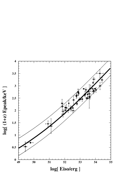
Figure 1: Left to right and top to bottom (a to d): a) The $[E_{p},E_{\gamma}^{\rm iso}]$ correlation of Eq. (4). b) The $[E_{p},L_{p}^{\rm iso}]$ correlation of Eq. (5). c) The $[t_{\rm min}^{\rm rise},L_{p}^{\rm iso}]$ correlation of Eq. (6). d) The $[V,L_{p}^{\rm iso}]$ correlation of Eq. (7). The dotted ‘variance lines’ are to guide the eye, they are not always symmetric about the best fit.

an expression with two parameters ($E_{p}^{0}$, $E_{0}^{\rm iso}$); like the correlation $E_{p}=a\,[E_{\gamma}^{\rm iso}]^{b}$ (see, e.g., Amati 2006a,b,c), whose power behaviour is arbitrary. A fit to Eq. (4) is shown in Fig. 1a. The variances around the mean trends of all the correlations we study have roughly log-normal distributions. Thus our fits are to the logarithms of the observed quantities.

The number fluence of a GRB is proportional to $\delta^{2}$, its energy fluence to $\delta^{3}$. The individual-photon energies are $\propto\delta\,\gamma$. All these facts imply that one expects most observed events to correspond to small $\theta$ (though obviously not to $\theta\simeq 0$, a set of null solid angle). Small $\theta$ means large $E_{p}$ and $E_{\gamma}^{\rm iso}$, approximately related by $(1\!+\!z)E_{p}\propto[E_{\gamma}^{\rm iso}]^{2/3}$. The expectation is supported by the data in Fig. 1a. These comments on the $[E_{p}\,,E_{\gamma}^{\rm iso}]$ correlation and the way it is derived are extensible to the other correlations we shall discuss, e.g., to the $[E_{p}\,,L_{p}^{\rm iso}]$ correlation predicted and tested in Dar & De Rújula (2001, 2004). Given Eq. (2) and in analogy with Eq. (4), we expect (Dado et al. 2006):

$$(1+z)\,E_{p}\simeq E_{p}^{0}\,\left\{[(1+z)^{2}\,L_{p}^{\rm iso}/L_{p}^{0}]^{1/4}+[(1+z)^{2}\,L_{p}^{\rm iso}/L_{p}^{0}]^{1/2}\right\}.$$ (5)

This correlation is akin to the one proposed by Yonetoku et al. (2004), but its power behaviour is not arbitrary.

To derive the other correlations we shall confront with data, we must recall the CB-model expectations for pulse rise-times and event variabilities, and derive the one for the lag-time. But Eqs. (2,3) allow us to anticipate the results:

$${t_{\rm min}^{\rm rise}\,(1+z)^{-1}}=t_{0}\left\{\left[(1+z)^{2}\,L_{p}^{\rm iso}/L_{p}^{0}\right]^{1\over 4}+\left[(1+z)^{2}\,L_{p}^{\rm iso}/L_{p}^{0}\right]^{1\over 2}\right\}^{-1}$$ (6)

$${(1+z)\,V}=V_{0}\;\left\{\left[(1+z)^{2}\,L_{p}^{\rm iso}/L_{p}^{0}\right]^{1\over 4}+\left[(1+z)^{2}\,L_{p}^{\rm iso}/L_{p}^{0}\right]^{1\over 2}\right\}$$ (7)

$${t_{\rm lag}\,(1+z)^{-2}}=t_{0}\left\{\left[(1+z)^{2}\,L_{p}^{\rm iso}/L_{p}^{0}\right]^{1\over 2}+\left[(1+z)^{2}\,L_{p}^{\rm iso}/L_{p}^{0}\right]^{1}\right\}^{-1}$$ (8)

The predictions of Eqs. (4) to (8) are tested in Figs. 1 and 2a. The data are from Schaefer (2006); values of $E_{0}^{\rm iso}$ and data for some extra GRBs at low $E_{0}^{\rm iso}$ and $E_{p}$ (which could be classified as X-ray flashes) are from Amati (2006a,b,c). All results are satisfactory.

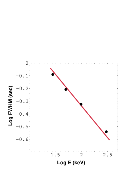
Figure 2: Left to right and top to bottom (a to d): a) The $[t_{\rm lag},L_{p}^{\rm iso}]$ correlation of Eq. (8). b) The $[t_{\rm lag},E_{p}]$ correlation of Eq. (9). c) The $[E_{\gamma}^{\rm iso},L_{p}^{\rm iso}]$ correlation of Eq. (9). d) The correlation between $t_{\rm FHHM}$ and BATSE $E$-channel of Section 6. The dotted ‘variance lines’ are to guide the eye, they are not always symmetric about the best fit.

Two observables ($L_{p}^{\rm iso}$ and $t_{\rm min}^{\rm rise}$) reflect fixed values of $\gamma$ and $\delta$, since they refer to a particular pulse in a GRB light curve, not necessarily the same one. For multi-pulse GRBs, the other observables reflect averages over the various pulses. Single-peak correlations should be tighter than the ones we have discussed, but properly analized data are not available. We also expect correlations between two multi-pulse-averaged observables to be tighter than those between a multi-pulse observable and a single-pulse one. The only correlation of the former type in Figs. 1 and 2 is that between $E_{p}$ and $E_{\gamma}^{\rm iso}$ in Fig. 1a; it is indeed the tightest.

The correlations we have discussed are not the simplest ones the CB model suggests. Indeed, it follows from Eqs. (2,3) that:

$$t_{\rm lag}\propto E_{p}^{-2},\;\;\;\;\;E_{\gamma}^{\rm iso}\propto[(1+z)^{2}\,L_{p}^{\rm iso}]^{3/4},\;\;\;\;\;V\propto E_{p},\;\;\;\;\;t_{\rm rise}\propto E_{p}^{-1}.$$ (9)

These relations involve just one parameter: the proportionality factor, and deserve to be studied, even if they add no significance to the results, for they are redundant with the correlations we have already discussed. The first two predictions in Eqs. (9) are shown in Figs. 2b,c. The correlations of $V$ and $t^{\rm rise}_{\rm min}$ with $E_{p}$ are less informative, not only because the first two of these observables are of a somewhat debatable significance, but because the dynamical ranges of $V$, $t^{\rm rise}_{\rm min}$ and $E_{p}$ span $\sim 2$ orders of magnitude, while the data on $L_{p}^{\rm iso}$, $E_{\gamma}^{\rm iso}$ and $t_{\rm lag}$ span $\sim 3$ times as many.

4 Variability and minimum rise-time

In the CB model there are two a priori time scales determining the rise-time and duration of a pulse: the time it takes a CB to expand to the point at which it becomes transparent to radiation and the time it takes it to travel to a distance from which the remaining of its path is transparent to $\gamma$ rays (Dar & De Rújula 2004). These two times are, for typical parameters, of the same order of magnitude. We discuss the second time scale here, for it is the one naturally leading to larger variabilities and differences in rise-time.

The $\gamma$ rays of a GRB’s pulse must traverse the pre-SN wind material remaining upstream of their production point, at a typical distance of $r={\cal{O}}(10^{16}\,\rm cm)$ from the parent SN. At these ‘short’ distances, the observed circumburst material is located in layers whose density decreases roughly as $1/r^{2}$ and whose typical $\rho\,r^{2}$ is large: $\sim 10^{16}\,{\rm g\,cm}^{-1}$ (Chugai et al. 2003; Chugai & Danzinger 2003). Compton absorption in such a wind implies that a pulse of a GRB initially rises with time as ${\rm Exp}[-(t^{w}_{tr}/t)^{2}]$, where (Dar & De Rújula 2004):

$${t^{w}_{tr}\over 1+z}=(0.13\,{\rm s})\;{\rho\,r^{2}\over 10^{16}\,{\rm g\,cm}^{-1}}\;{10^{6}\over\gamma\,\delta}.$$ (10)

The values of $\delta\,\gamma$ may differ for the different CBs (pulses) of a GRB even if they are emitted in precisely the same direction, which need not be the case, e.g. if the emission axis precesses. The minimum rise-time, $t_{\rm rise}$, used as a variability measure in Schaefer (2006), satisfies Eq. (10), and was used in Fig. 1c.

The result in Eq. (10) is for an ideal spherically-symmetric wind. Actual wind distributions are layered and patchy, implying an in-homogeneous distribution of the glory’s light density. Since the number of photons Compton up-scattered by the CB is proportional to this density, the inhomogeneities would directly translate into a variability on top of a smooth pulse shape, which reflects the average density distribution of the wind-fed medium. This corresponds to a source of variability that, as a function of $\delta$, $\gamma$ and $z$, behaves as the inverse of $t^{w}_{tr}$, the form used for $V$ in Eq. (2) and Fig. 1d (in the CB model, the deviations from a smooth behaviour observed in some optical and X-ray AGs also trace the inhomogeneities in the density of the interstellar medium; see Dado et al. 2003a, 2006). There are many ways to define the variability of a GRB; variations of the sort we have described are the ones studied by Schaefer (2006). The data in Figs. 1c,d are from his analysis and definitions.

5 The lag-time

In the CB model a pulse’s $\gamma$-ray number flux as a function of energy and time is of the form (Dar & De Rújula, 2004):

$$N(E,t)\equiv{d^{2}N\over dE\,dt}={dN_{1}(E,t)\over dE}\,{dN_{2}(t)\over dt}\,.$$ (11)

The function $dN_{2}/dt$ is well approximated by ${\rm Exp}[-(t^{w}_{tr}/t)^{2}]\,\{[1-{\rm Exp}[-(t^{w}_{tr}/t)^{2}]\}$, with $t^{w}_{tr}$ as in Eq. (10). The predicted shape of $dN_{1}/dE$ is amazingly similar to that of ‘Band’s’ phenomenological spectrum and has a weak time-dependence that makes the spectrum within a pulse soften with time, in a time of order $t^{w}_{tr}$. The energies $E$ in $dN_{1}/dE$ scale with $T$:

$$T\equiv{4\over 3}\;T_{i}\;{\gamma\;\delta\over 1+z}\;\,\langle 1+\cos\theta_{i}\rangle,$$ (12)

where $\theta_{i}$ is the angle of incidence of a glory’s photon onto the CB (in the SN rest system) and $T_{i}$ is the pseudo-temperature in the thin thermal-bresstrahlung spectrum $[{\rm Exp}(-E_{i}/T_{i})]/E_{i}$ of the glory’s light. We conclude that $N(E,t)=F\left({E/T}\;,{t/t^{w}_{tr}}\right)$ with $F$ a predicted function. This implies that

$$t_{\rm rise}(E)=t^{w}_{tr}\;G(E/T),$$ (13)

with $G(x)$ a slowly-varying function of $x$ (a fact that can be traced back to the time dependence of $dN_{1}/dE$ being much slower than that of $dN_{2}/dt$).

Let $t_{\rm rise}(E_{i})$ be the rise-time of a pulse at a given $\gamma$-ray energy $E_{i}$. The lagtime is defined and approximated as:

$$t_{\rm lag}\simeq t_{\rm rise}(E_{2})-t_{\rm rise}(E_{1})\approx\Delta\,E\;{dt_{\rm rise}\over dE}\;,$$ (14)

where $\Delta E$ is generally taken to be a fixed energy interval between two ‘channels’ in a given detector. Use Eqs. (13, 14) to deduce that:

$$t_{\rm lag}\approx t^{w}_{tr}\,{dG\over dE}\,\Delta\,E\propto{t^{w}_{tr}\over T}\,\Delta\,E$$ (15)

where, on dimensional grounds, we used $dG/dE\propto 1/T$. It follows from Eqs. (12,10) that:

$$t_{\rm lag}\propto{t^{w}_{tr}\over T}\propto{(1+z)^{2}\over\delta^{2}\,\gamma^{2}}\,,$$ (16)

the result announced in Eq. (3) and used in Fig. 2a.

6 The duration of a GRB pulse

Some correlations do not follow from comparisons of $\gamma$ and $\delta$ dependences. One of them (Dar & De Rújula 2004) is the following. As the CB reaches the more transparent outskirts of the wind, its ambient light becomes increasingly radially directed, so that the average $1+\cos\theta_{i}$ in Eq. (12) will tend to $0$ as $1/r^{2}\propto 1/t^{2}$. Since the (exponential) rise of a typical pulse is much faster than its (power) decay, the width of a peak is dominated by its late behaviour at $t>t_{tr}$. At such times, $T\propto 1/t^{2}$ in Eq. (12), so that $dN/dE$ is, approximately, a function of the combination $E\,t^{2}$. Consequently, the width of a GRB pulse in different energy bands is: $\Delta t\propto E^{-1/2}$, in agreement with the observation, $t_{{}_{\rm FWHM}}\propto E^{-0.43\pm 0.10}$ , for the average FWHM of peaks as a function of the energies of the four BATSE channels (Fenimore et al. 1995, Norris et al. 1996). This correlation is shown in Fig. 2d.

7 Conclusions

The CB model is very successful in its description of all properties of the pulses of long-duration GRBs (Dar & De Rújula 2004). We have extended our previous discussions of one of these properties: the correlations between pairs of observables. We have analyzed a wealth of newly available data and derived predictions for some observables which we had not studied before. Although our predictions are expected to be better satisfied for individual pulses, the results are very satisfactory even when applied to entire GRBs: all of the predicted trends agree with the observations. The correlations we have discussed have a common and simple physical basis: relativistic kinematics and Compton scattering. The viewing angle $\theta$ is the most crucial parameter underlying the correlations, and determining the properties of GRBs and their larger-$\theta$ counterparts, X-ray flashes (Dar & De Rújula 2004, Dado et al. 2004).

Acknowledgements. This research was supported in part by the Helen Asher Space Research Fund and the Institute for Theoretical Physics at the Technion Institute. ADR thanks the Institute for its hospitality.

8 Appendix

In this Appendix, and in the example of the $[E_{p},\,E_{\gamma}^{\rm iso}]$ correlation, we prove in detail the “double-power” nature of many of the correlations predicted by the CB model.

For a typical angle of incidence (Dar & De Rújula 2004), the energy of a Compton up-scattered photon from the SN glory is Lorentz and Doppler boosted by a factor $\sim\!\gamma\,\delta/2$ and redshifted by $1\!+\!z$. The peak energy $E_{p}$ of the GRB’s $\gamma$-rays is related to the peak energy, $\epsilon_{p}\!\sim\!1$ eV, of the glory’s light by:

$$(1+z)\,E_{p}\simeq{\gamma\,\delta\,\epsilon_{p}\over 2}\simeq(500\;{\rm keV})\;{\gamma\,\delta\over 10^{6}}\,{\epsilon_{p}\over 1\;\rm eV}\;.$$ (17)

The spherical equivalent energy, $E_{\gamma}^{\rm iso}$, is (Dar & De Rújula 2004, Dado et al. 2006b):

$$E_{\gamma}^{\rm iso}\simeq{\delta^{3}\,L_{{}_{\rm SN}}\,N_{{}_{\rm CB}}\,\beta_{s}\over 6\,c}\,\sqrt{\sigma_{{}_{\rm T}}\,N_{b}\over 4\,\pi}\sim(3.8\!\times\!10^{53}\,{\rm erg})\,{\delta^{3}\over 10^{9}}\,{L_{{}_{\rm SN}}\over L_{{}_{\rm SN}}^{\rm bw}}\,{N_{{}_{\rm CB}}\over 6}\,\beta_{s}\sqrt{N_{b}\over 10^{50}}\;,$$ (18)

where $L_{{}_{\rm SN}}$ is the mean SN optical luminosity just prior to the ejection of CBs, $N_{{}_{\rm CB}}$ is the number of CBs in the jet, $N_{b}$ is their mean baryon number, $\beta_{s}$ is the comoving early expansion velocity of a CB (in units of $c/\sqrt{3}$), and $\sigma_{{}_{\rm T}}$ is the Thomson cross section. The early SN luminosity required to produce the mean isotropic energy, $E_{\gamma}^{\rm iso}\!\sim\!4\!\times\!10^{53}$ erg, of ordinary long GRBs is $L_{{}_{\rm SN}}^{\rm bw}\!\simeq\!5\!\times\!10^{42}\,{\rm erg\,s^{-1}}$, the estimated early luminosity of SN1998bw.

The explicit proportionality factors in the relations $E_{p}\propto\gamma\,\delta$ and $E_{\gamma}^{\rm iso}\propto\delta^{3}$ are given by Eqs. (17,18). Let us first consider them fixed at their typical values. The typical $[\gamma,\,\delta]$ domain of observable GRBs is then the one shown in Fig. 3a. The observed values of $\gamma$ are fairly narrowly distributed around $\gamma\!\sim\!10^{3}$ (Dado et al. 2003a, Dar & De Rújula, 2004), as in the blue strip of the figure. The $[\gamma,\,\delta]$ domain is also limited by a minimum observable isotropic energy or fluence (both $\propto\,\delta^{3}$), by a minimum observable peak energy, and by the line $\theta=0$ or, if one takes into account that phase space for observability diminishes as $\theta\to 0$, by a line corresponding to a minimum fixed $\theta$. The elliptical “sweet spot” in Fig. 3a is the region wherein GRBs are most easily detectable, particularly in pre-Swift times. In the CM model X-ray Flashes are GRBs seen at a relatively large $\theta\gamma$ (Dar & De Rújula, 2004, Dado et al. 2004) they populate the region labeled XRF in the figure, above the fixed $\gamma\theta$ line or to the left of the fixed $E_{p}$ line.

The blue line in Fig. 3d is the contour of the blue domain of Fig. 3a, shown in the $[\gamma\delta,\,\delta^{3}]$ plane of the $[E_{p},\,E_{\gamma}^{\rm iso}]$ correlation. At low values of these quantities, the correlation is $E_{p}\,\propto\!(E_{\gamma}^{\rm iso})^{1/3}$. At the opposite extreme, the expected power is half-way between 1/3 and 2/3. But there is another effect increasing this expectation to $\sim\!2/3$.

A CB that is expanding, in its rest system, at a speed of relativistic sound ($\beta_{\rm exp}\!=\!\beta_{s}$) –or at the speed of light ($\beta_{\rm exp}\!=\!1$)– subtends a non-vanishing angle from its point of emission. In the SN rest system, this (half-)angle is $\theta_{{}_{\rm CB}}\!=\!\beta_{\rm exp}/\gamma$. At a fixed observer’s angle, $\theta$, the value of $\delta$ and $\delta^{3}$ entering Eqs. (17,18) are not the “naive” ones of Eq. (1), but are averages, $\langle\delta\rangle$ and $\langle\delta^{3}\rangle$, over the CB’s non-vanishing surface. In Fig. 3b we show function $\langle\delta(\theta\gamma)\rangle$, for fixed $\gamma$ and $\theta_{{}_{\rm CB}}\!=\!1/\gamma$ (the result is very similar for $\beta_{\rm exp}=1/\sqrt{3}$). This figure is easy to interpret: for $\theta\gg\theta_{{}_{\rm CB}}$, the CB is effectively point-like and $\langle\delta(\theta\gamma)\rangle\to\delta$. At the opposite extreme, $\theta\ll\theta_{{}_{\rm CB}}$, the observer’s angle is immaterial and $\langle\delta(\theta\gamma)\propto\gamma$. The consequences of this fact on the $[E_{p},\,E_{\gamma}^{\rm iso}]$ correlation can be seen in Fig. 3c, where we have plotted $E_{p}\!\propto\!\gamma\langle\delta\rangle$ versus $E_{\gamma}^{\rm iso}\!\propto\!\langle\delta^{3}\rangle$, at fixed $\gamma$. The $E_{p}(E_{\gamma}^{\rm iso})$ functional dependence smoothly evolves from a 1/3 to a 2/3 power. We plot in Fig. 3d, as the banana-like dashed line, the border of the blue domain of Fig. 3a, taking into account the geometrical effect we just described. The result is an $[E_{p},\,E_{\gamma}^{\rm iso}]$ correlation with an index varying from 1/3 to $\sim\!2/3$.

Finally, we may consider the effect of varying the proportionality factors in Eqs. (17,18) around their reference values. This results in a superposition of banana-like domains, the general behaviour of which we have approximated by the $[E_{p},\,E_{\gamma}^{\rm iso}]$ correlation of Eq. (4). Similar considerations apply to all the other two-power correlations that we have studied.

         

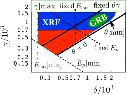
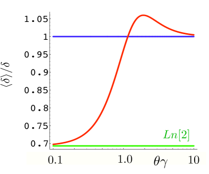
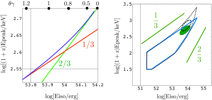
Figure 3: Left to right and top to bottom: a) The $[\delta,\,\gamma]$ domain. b) The ratio $\langle\delta\rangle/\delta$ of average to naive Doppler shifts for a (Lorentz-contracted) disk-like CB of angular size $1/\gamma$ (in the SN rest system), as a function of $\theta\,\gamma$. c) $E_{p}$ versus $E_{\gamma}^{\rm iso}$ for the same CB, at fixed $\gamma$. d) Contours of $E_{p}$ versus $E_{\gamma}^{\rm iso}$ for an ensemble of CBs whose values of $[\delta,\,\gamma]$ are in the blue domain of Fig. 3a. The continuous (blue) contour does not take into account the non-point-like character of CBs. The dashed contour does.

References

- (1) Amati, L., 2006a, MMRAS, 372, 233
- (2) Amati, L. 2006b, astro-ph/0601553
- (3) Amati, L., 2006c, astro-ph/0611189
- (4) Chugai, N.N. & Danziger, I.J. 2003, Astron. Lett. 29 649
- (5) Chugai, N.N. et al. Proceedings of IAU Colloquium 192, it Supernovae, eds. J. M. Marcaide and K. W. Weiler
- (6) Dado, S., Dar, A. & De Rújula, A. 2002, A&A, 388, 1079
- (7) Dado, S., Dar, A. & De Rújula, A. 2003a, A&A, 401, 243
- (8) Dado, S., Dar, A. & De Rújula, A. 2003b, ApJ, 594, L89
- (9) Dado, S., Dar, A. & De Rújula, A. 2004, A&A, 422, 381
- (10) Dado, S., Dar, A. & De Rújula, A. 2006a, ApJ, 646, L21
- (11) Dado, S., Dar, A., De Rújula and Plaga, R., astro-ph/0611161
- (12) Dar, A. & Plaga, R. 1999, A&A, 349, 259
- (13) Dar, A. & De Rújula, A. 2000, astro-ph/0008474
- (14) Dar, A. & De Rújula, A. 2001, astro-ph/0012227
- (15) Dar, A. & De Rújula, A. 2004, Physics Reports, 405, 203
- (16) De Rújula, A, 1987, Phys. Lett. 193, 514
- (17) Fenimore, E. E., in ’t Zand, J. J. M., Norris, J. P., Bonnell, J. T. & Nemiroff, R. J. 1995, ApJ, 448, L101
- (18) Fenimore, E.E. & Ramirez-Ruiz, E. 2000, astro-ph/0004176
- (19) Guidorzi, C., et al. 2006, MNRAS, 371, 843
- (20) Norris, J. P., Nemiroff, R. J., Bonnell, J. T., Scargle, J. D., Kouveliotou, C., Paciesas, W. S., Meegan, C. A. & Fishman, G. J. 1996, ApJ, 459, 393
- (21) Plaga, R. 2001, A&A, 370, 351
- (22) Reichart, D. E., et al. 2001, ApJ, 552, 57
- (23) Schaefer, B. E., astro-ph/0612285
- (24) Shaviv, N. J., Dar, A. 1995, ApJ, 447, 863
- (25) Yonetoku, D., et al. 2004, ApJ. 609, 935