Stochastic background from inspiralling double neutron stars

Abstract

We review the contribution of extra galactic inspiralling double neutron stars, to the LISA astrophysical gravitational wave foreground.

Using recent fits of the star formation rate, we show that sources beyond $z_{*}=0.005$ contribute to a truly continuous background, which may dominate the LISA instrumental noise in the range $3\simeq 10^{-4}$ - $1\times 10^{-2}$ Hz and overwhelm the galactic WD-WD confusion noise at frequencies larger than $\nu_{o}\simeq 2\times 10^{-3}$.

I Introduction

Compact neutron star binaries are among the most promising sources of gravitational waves. At low frequencies, the continuous inspiral signal may be detectable by the space antenna LISA, while ground based interferometers such as VIRGO Bradaschia et al. (1990), LIGO Abramovici et al. (1992), GEO Hough (1992) or TAMA Kuroda et al. (1997), are expected to detect the last few minutes prior coalescence, at frequencies up to 1.4-1.6 kHz.

In a first paper de Freitas Pacheco et al. (2005) (hereafter paper I), we have investigated the high frequency signal and its detection with the first generations of ground based detectors. Using new estimates of the mean merging rate in the local universe, that account for the galactic star formation history derived directly from observations and include the contribution of elliptical galaxies, we predict a detection every 148 and 125 years in the volume probed by initial VIRGO and LIGO, and up to 6 detections per year in their advanced configuration.

In a second paper Regimbau & de Freitas Pacheco (2006) (hereafter paper II), we used numerical simulations to estimate the gravitational wave emission produced by the superposition of unresolved extra-galactic sources. As in paper I, we were interested in the few sixteen minutes before the last stable orbit is reached, when more than 96% of the gravitational wave energy is released and when the frequency evolves in the range 10-1500 Hz, covered by ground based interferometers. We find that above the critical redshift $z_{*}=0.23$, the sources produce a truly continuous background, with a maximal gravitational density parameter of $\Omega_{gw}\simeq 1.1\times 10^{-9}$ around 670 Hz. The signal is below the sensitivity of the first generation of ground based detectors but could be detectable by the next generation. Correlating two coincident advanced-LIGO detectors or two third generation EGO interferometers, we derived a S/N ratio of 0.5 and 10 respectively.

In this article, we extend our previous simulations to investigate the stochastic background from the early low frequency inspiral phase. Estimates of the emission from the various population of compact binaries (see for instance Evans et al. (1987); Hils et al. (1990); Bender & Hils (1997); Postnov K.A. & Prokhorov M.E (1998); Nelenan et al. (2001); Timpano et al. (2005) for the galactic contribution and Schneider et al. (2001); Farmer & Phinney (2002); Cooray (2004) for the extra-galactic contribution) or from captures by supermassive black holes (Barack (2004)), which represent the main source of confusion noise for LISA, are of crucial interest for the development of data analysis strategies. The paper will be organized as follow. In II., we describe the simulations of the DNS population, in III. the contribution of inspiralling DNS to the stochastic background is calculated and compared to the LISA instrumental noise and to the WD-WD galactic foreground. Finally, in IV. the main conclusions are summarized.

II Simulations of the DNS population

To generate a population of DNSs (each one characterized by its redshift of formation and coalescence timescale) we follow the same procedure as in paper II, to which the reader is referred for a more detailed description.

The redshift of formation is randomly selected from the probability distribution Coward et al. (2002):

$$P_{f}(z_{f})=\frac{R_{zf}(z_{f})}{R_{p}}$$ (1)

constructed by normalizing the differential DNS formation rate,

$$R_{zf}(z_{f})=\frac{dR_{f}(z_{f})}{dz_{f}}$$ (2)

The normalization factor in the denominator corresponds to the rate at which massive binaries are formed in the considered redshift interval, e.g.,

$$R_{p}=\int_{0}^{6}(dR_{f}(z_{f})/dz_{f})dz_{f},$$ (3)

which numerically gives $R_{p}=0.044$ s^-1 in the two cosmic star formation rate adopted in this paper.

The formation rate of massive binaries per redshift interval eq. 2 writes :

$$R_{zf}(z_{f})=\lambda_{p}\frac{R^{*}_{f}(z_{f})}{1+z_{f}}{\frac{{dV(z_{f})}}{{dz_{f}}}}$$ (4)

where $R^{*}_{f}(z)$ is the cosmic star formation rate (SFR) expressed in M_⊙ Mpc^-3yr^-1 and $\lambda_{p}$ is the mass fraction converted into DNS progenitors. Hereafter, rates per comoving volume will always be indicated by the superscript ’*’, while rates with indexes “z_f” or “z_c” refer to differential rates per redshift interval, including all cosmological factors. The (1+z) term in the denominator of eq. 4 corrects the star formation rate by time dilatation due to the cosmic expansion.

The element of comoving volume is given by

$$dV=4\pi r^{2}\frac{c}{H_{o}}\frac{dz}{E(\Omega_{i},z)}$$ (5)

with

$$E(\Omega_{i},z)=[\Omega_{m}(1+z)^{3}+\Omega_{v}]^{1/2}$$ (6)

where $\Omega_{m}$ and $\Omega_{v}$ are respectively the present values of the density parameters due to matter (baryonic and non-baryonic) and vacuum, corresponding to a non-zero cosmological constant. Throughout this paper, the 737 flat cosmology Rao et al. (1990), with $\Omega_{m}$ = 0.30, $\Omega_{v}$ = 0.70 and Hubble parameter H₀ = $70\,\mathrm{km\,s}^{-1}\mathrm{Mpc}^{-1}$ Spergel et al. (2003) is assumed.

Recent measurements of galaxy luminosity function in the UV (SDSS, GALEX, COMBO17) and FIR wavelengths (Spitzer Space Telescope), after dust corrections and normalization, allowed to refine the previous models of star formation history, up to redshift $z\simeq 6$, with tight constraints at redshifts $z<1$. In our computations, we consider the recent parametric fits of the form of Cole et al. (2003), provided by Hopkins & Beacom (2006), constrained by the Super Kamiokande limit on the electron antineutrino flux from past core-collapse supernovas. It is worth mentioning that the final results are not significantly different if we adopt, as in paper II, the SFR given in Porciani & Madau (2001).

Throughout this paper, we assume that the parameter $\lambda_{p}$ does not change significantly with the redshift and can be considered as a constant. In fact, this term is the product of three other parameters, namely,

$$\lambda_{p}=\beta_{NS}f_{b}\lambda_{NS}$$ (7)

where $\beta_{NS}$ is the fraction of binaries which remains bounded after the second supernova event, $f_{b}$ is the fraction of massive binaries formed among all stars and $\lambda_{NS}$ is the mass fraction of neutron star progenitors. From paper I we take $\beta_{NS}$ = 0.024 and $f_{b}$ = 0.136.

Hopkins & Beacom (2006) investigated the effect of the initial mass function (IMF) assumption on the normalization of the SFR. They showed that top heavy IMFs are preferred to the traditional Salpeter IMF (Salpeter, 1995) and their fits are optimized for IMFs of the form:

$$\xi(m)\>\propto\begin{array}[]{ll}\frac{m}{m_{0}}^{-1.5}&\hbox{ for }0.1<m<m_{0}\\ \frac{m}{m_{0}}^{-\gamma}&\hbox{ for }m_{0}<m<100\\ \end{array}$$ (8)

with a turnover below $m_{0}=1$ M_⊙, and normalized within the mass interval 0.1 - 100 M_⊙ such as $\int m\xi(m)dm$ = 1.

In this paper, we assume $\gamma=2.35$ (A modified Salpeter), but taking $\gamma=2.2$ (Baldry & Glazebrook (2003)) would not change the final results significantly. To be consistent with the adopted models of the SFR, we follow Hopkins & Beacom (2006) and assume a minimal initial mass of 8 M_⊙ for NS progenitors, the upper mass being 40 M_⊙. It results finally , $\lambda_{NS}=\int_{8}^{40}\xi(m)dm=9\times 10^{-3}$ M${}_{\odot}^{-1}$.

The next step consists to estimate the redshift $z_{b}$ at which the progenitors have already evolved and the system is now constituted by two neutron stars. This moment fixes also the beginning of the inspiral phase. If $\tau_{b}$ ($\approx 10^{8}$ yr) is the mean lifetime of the progenitors (average weighted by the IMF in the interval 8-40 M_⊙) then

$$z_{b}=z_{f}-H_{0}\tau_{b}(1+z_{f})E(z_{f})$$ (9)

Once the beginning of the inspiral phase is established, the redshift at which the coalescence occurs should now be estimated. The duration of the inspiral depends on the orbital parameters and the neutron star masses. The probability for a given DNS system to coalesce in a timescale $\tau$ was initially derived by de Freitas Pacheco (1997) and confirmed by subsequent simulations Vincent (2002); de Freitas Pacheco et al. (2005) and is given by

$$P(\tau)=B/\tau$$ (10)

Simulations indicate a minimum coalescence timescale $\tau_{0}=2\times 10^{5}$ yr and a considerable number of systems having coalescence timescales higher than the Hubble time. The normalized probability in the range $2\times 10^{5}$ yr up to 20 Gyr implies $B=0.087$. Therefore, the redshift $z_{c}$ at which the coalescence occurs is derived by solving the equation

$$\tau=\tau(z_{c},z_{b})$$ (11)

where

$$\tau(a,b)=\int_{a}^{b}\frac{dz}{H_{0}(1+z)E(z)}$$ (12)

III The Gravitational Wave Background

Compared with the previous study, slight complications arise when calculating the spectral properties of the signal. In paper II, we were interested in the signal emitted between 10-1500 Hz, which duration in the source frame is short enough, less than 1000 s, to be considered as a burst located at the redshift of coalescence. Now, as we are looking at inspiral phase in the LISA frequency window ($10^{-4}-0.1$ Hz), the evolution of the redshift of emission with frequency must be taken into account. For the same reason, the critical redshift at which the population of DNSs constitute a truly continuous background can’t be determined by simply solving the condition $D(z)>1$, where D is the duty cycle defined as the ratio of the typical duration of a single burst $\bar{\tau}$ to the average time interval between successive events (see paper II). Instead, we remove the brightest sources, lying in the close Universe, where the distribution of galaxies is expected to be highly anisotropic, in particular due to the strong concentration of galaxies in the direction of the Virgo cluster and the Great Attractor (see paper I), and where the density is well below the average value derived from the SFR (de Freitas Pacheco (2006)). In a second step, we verify that the resulting background is continuous, by using both Jaque Bera and Lilliefors gaussianity tests with significant level $\alpha=0.05$ over a set of 100 realizations.

For each realization, the number of simulated DNSs corresponds to the expected number of extragalactic DNSs observed today and is derived as,

$$N_{p}=\int_{0}^{6}N(z)dz$$ (13)

The DNSs present at redshift z were formed at $z^{\prime}_{b}\geq z$, with a coalescence time larger than the cosmic time between $z^{\prime}_{b}$ and z. Thus,

$$N(z)=\int_{z}^{6}R_{zc}(z^{\prime})\eta(z^{\prime})dz^{\prime}$$ (14)

where

$$\eta(z^{\prime})=\int_{\tau_{min}}^{\tau_{max}}P(\tau)d\tau$$ (15)

with $\tau_{max}$= 20 Gyr and $\tau_{min}$=Max($2\times 10^{5}$ yr;$\tau(z,z^{\prime}_{b})$), which gives $N_{p}\simeq 1.4\times 10^{6}$.

We obtain that after $z_{*}=0.005$, corresponding to the distance beyond the Virgo cluster ($\simeq 25$ Mpc), when the relative density fluctuations are $<0.5$ (de Freitas Pacheco (2006)), the background is continuous in the range $10^{-4}-0.1$ Hz. We consider also a more conservative threshold of $z_{*}=0.02$, corresponding to the distance beyond the Great Attractor ($\simeq 100$ Mpc), when the relative density fluctuations are $<0.05$ and when the Universe is expected to become homogeneous(de Freitas Pacheco (2006); Wu et al. ).

The gravitational flux in the observer frame produced by a given DNS is:

$$f_{\nu_{o}}=\frac{1}{4\pi d_{L}^{2}}\frac{dE_{gw}}{d\nu}(1+z_{e})$$ (16)

where $z_{e}$ is the redshift of emission, $d_{L}=(1+z_{e})r$ the distance luminosity, $r$ the proper distance, which depends on the adopted cosmology, ${dE_{gw}}/{d\nu}$ the gravitational spectral energy and $\nu=(1+z_{e})\nu_{o}$ the frequency of emission in the source frame.

In the quadripolar approximation and for a binary system with masses $m_{1}$ and $m_{2}$ in a circular orbit:

$$dE_{gw}/{d\nu}=K\nu^{-1/3}$$ (17)

where the fact that the gravitational wave frequency is twice the orbital frequency was taken into account. Then

$$K=\frac{(G\pi)^{2/3}}{3}\frac{m_{1}m_{2}}{(m_{1}+m_{2})^{1/3}}$$ (18)

Taking $m_{1}=m_{2}=1.4$ M_⊙, one obtains $K=5.2\times 10^{50}$ erg Hz^-2/3.

The redshift of emission is derived by solving the relation Schneider et al. (2001):

$$\nu^{-8/3}=\nu_{LSO}+K^{\prime}(\tau(z_{b},z_{e}))$$ (19)

where

$$K^{\prime}=\frac{(256\pi^{8/3}G^{5/3})}{5c^{5}}$$ (20)

(or numerically $K^{\prime}=67.83$ yr^-1), and where the time spent between redshifts $z_{e}$ and $z_{b}$ is given by:

$$\tau(z_{b},z_{e})=\tau-\int_{z_{c}}^{z_{e}}\frac{dz}{(1+z)E(z)}$$ (21)

III.1 Properties of the background

The spectral properties of the stochastic background are characterized by the dimensionless parameter Ferrari et al. (1999):

$$\Omega_{gw}(\nu_{o})=\frac{1}{c^{3}\rho_{c}}{\nu_{o}}F_{\nu_{o}}$$ (22)

where $\nu_{o}$ is the wave frequency in the observer frame and $\rho_{c}$ the critical mass density needed to close the Universe, related to the Hubble parameter $H_{0}$ by,

$$\rho_{c}=\frac{3H_{o}^{2}}{8\pi G}$$ (23)

$F_{\nu_{o}}$ is the gravitational wave flux at the observer frequency (given here in erg cm^-2Hz^-1s^-1) $\nu_{o}$, integrated over all sources above the critical redshift $z_{*}$, namely

$$F_{\nu_{o}}=\int_{z_{*}}^{z_{\max}}f_{\nu_{o}}dR_{c}(z)$$ (24)

In our simulations, the integrated gravitational flux is calculated by summing individual fluences (eq. 16), scaled by the ratio between the total formation rate of progenitors (eq. 3) and the number of simulated massive binaries, as:

$$F_{\nu_{o}}=\frac{R_{p}}{N_{p}}\sum_{i=1}^{N_{p}}f_{\nu_{o}}^{i}$$ (25)

Figure 1 shows the density parameter $\Omega_{gw}$ as a function of the observed frequency averaged over 10 simulations. The continuous line corresponds to sources located beyond the critical redshift to have a continuous background, $z_{*}=0.005$ (or $d\simeq 25$ Mpc), while the dashed line corresponds to the more conservative estimate, with a cutoff at $z_{*}=0.02$ (or $d\simeq 100$ Mpc). After a fast increase below $\simeq 5\times 10^{-5}$ Hz, $\Omega_{gw}$ increases as $\nu_{o}^{2/3}$ to reach $\Omega_{gw}\simeq 3\times 10^{-10}$ at 0.1 Hz for $z_{*}=0.005$ ($\Omega_{gw}\simeq 10^{-10}$ for $z_{*}=0.02$). This is one order of magnitude larger than the previous predictions by Schneider et al. (2001).

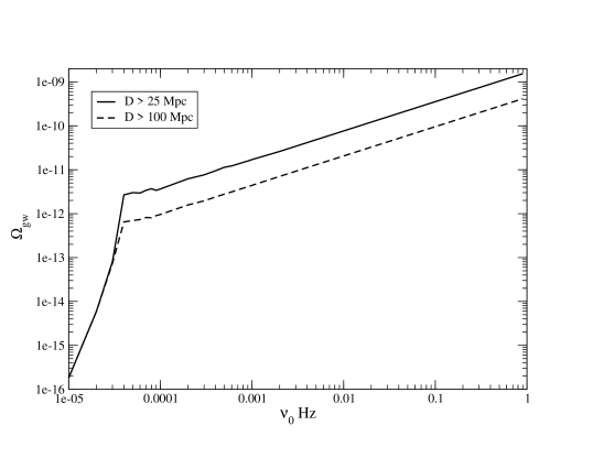
Figure 1: Spectrum of the expected gravitational energy density parameter $\Omega_{gw}$, corresponding to NS-NS inspirals occurring beyond $d\simeq 25$ Mpc (continuous curve) and $d\simeq 100$ Mpc (dashed curve).

III.2 consequences for LISA

Astrophysical backgrounds represent a confusion noise for LISA, which spectral density is given by Barack (2004):

$$S_{h}^{back}(\nu_{o})=\frac{3H_{0}^{2}}{2\pi^{2}}\frac{1}{\nu_{o}^{3}}\Omega_{\rm gw}(\nu_{o})$$ (26)

Figure 2 shows $S_{h}^{back}(\nu_{o})$ compared to the LISA sensitivity Larson (2000) and to the contribution of unresolved galactic WD-WD Hils et al. (1990); Larson (2000). The contribution from DNSs may dominate the LISA instrumental noise between $\simeq 3\times 10^{-4}$ - $10^{-2}$ Hz for $z_{*}=0.005$ ($\simeq 7\times 10^{-4}$ - $6\times 10^{-3}$ Hz for $z_{*}=0.02$) and the galactic WD-WD confusion noise after $\simeq 2\times 10^{-3}$. However, the resulting reduction in the sensitivity should be less than a factor 4 and thus shouldn’t affect significantly signal detection.

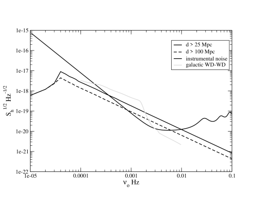
Figure 2: Gravitational strain in Hz^-1/2, corresponding to NS-NS inspirals occurring beyond $d\simeq 25$ Mpc (continuous curve) and $d\simeq 100$ Mpc (dashed curve), along with the LISA instrumental noise (black) and the galactic WD-WD foreground (light gray).

The critical redshift at which a single DNS can be resolved and detected by LISA (Figure 3) is at least one order of magnitude smaller ($z_{min}\simeq 3\times 10^{-4}$ at frequencies $\nu_{o}>0.01$) than our threshold to have a gaussian background $z_{*}=0.005$ (or $z_{*}=0.02$) . Sources lying between the two regimes are responsible for a non gaussian and non isotropic cosmic “popcorn” noise (see Coward & Regimbau (2006) for a recent review) that will be investigated in a further work. This contribution, which statistical properties differ from those of both the instrumental noise and the cosmological background, could be detected and removed by new data analysis techniques currently under investigation, such as the search for anisotropies Allen & Ottewill (1997) that can be used to create a map of the GW background Cornish (2001); Ballmer (2006), the maximum likelihood statistic Drasco & Flanagan (2003), or methods based on the Probability Event Horizon concept Coward & Burman (2005), which describes the evolution, as a function of the observation time, of the cumulated signal throughout the Universe.

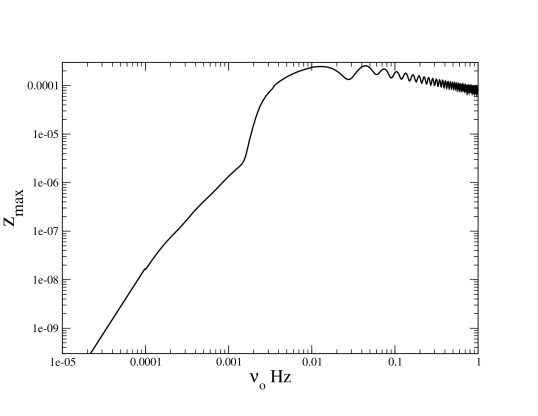
Figure 3: Maximal redshift as a function of the observed frequency, at which a single DNS can be detected by LISA after one year of integration and with a signal-to-noise ratio $S/R=5$. The galactic WD-WD foreground is taken into account in the LISA sensitivity.

IV Conclusions

In this paper, we have modelled the contribution of extra galactic inspiralling double neutron stars, to the to the astrophysical gravitational wave foreground, in the range of sensitivity of the space detector LISA.

Using a recent fit of the star formation rate Hopkins & Beacom (2006), optimized for a top heavy A modified Salpeter IMF, we show that sources beyond $z_{*}=0.005$ (or $z_{*}=0.02$ for a more conservative estimate) constitute a truly continuous background. We find that the density parameter $\Omega_{gw}$, after a fast increase below $\simeq 5\times 10^{-5}$ Hz, increases as $\nu_{o}^{2/3}$ to reach $\Omega_{gw}\simeq 3\times 10^{-10}$ ($\Omega_{gw}\simeq 10^{-10}$) at 0.1 Hz, which is one order of magnitude above the previous estimate of Schneider et al. (2001). As a result, the signal may dominate the LISA instrumental noise in the range $\simeq 3\times 10^{-4}$ - $10^{-2}$ Hz ($\simeq 7\times 10^{-4}$ - $6\times 10^{-3}$) and overwhelm the galactic WD-WD confusion noise at frequencies larger than $\nu_{o}\simeq 2\times 10^{-3}$. Sources located closer than $z_{*}$, but still too far to be detected by LISA, constitute a non gaussian and non isotropic cosmic “popcorn” noise, which will be investigated in a further work.

Acknowledgement

The author thanks J.A. de Freitas Pacheco and A. Spallicci for usefull discussions, which have improved the first versions of the paper.

References

- (1) D. Richstone et al., Nature 395, 14 (1998).
- Bradaschia et al. (1990) C. Bradaschia et al., Nucl. Instrum. Meth. A289, 518 (1990).
- Abramovici et al. (1992) A. Abramovici et al., Science 256, 325 (1992).
- Hough (1992) J. Hough, in Proceedings of the Sixth Marcel Grossmann Meeting, edited by H. Sato and T. Nakamura (Singapore: World Scientific, 1992), p. 192.
- Kuroda et al. (1997) K. Kuroda et al., in Proceedings of the International Conference on Gravitational Waves: Sources and Detectors, 1997 edited by I. Ciufolini and F. Fidecaro (Singapore: World Scientific, 1997), p. 1007.
- de Freitas Pacheco et al. (2005) J.A. de Freitas Pacheco, T. Regimbau, A. Spallicci and S. Vincent, IJMPD 15, 235 (2005).
- Regimbau & de Freitas Pacheco (2006) T. Regimbau and J.A. de Freitas Pacheco, Apj 642, 455 (2006).
- Evans et al. (1987) C.R. Evans,I. Iben and L. Smarr, Astrophys. J. 323, 129 (1987).
- Hils et al. (1990) D. Hils, P.L. Bender and R.F. Webbink R.F., ApJ 360, 75 (1990).
- Bender & Hils (1997) P.L. Bender and D. Hils D.. Class. Quant. Grav. 14, 1439 (1997).
- Postnov K.A. & Prokhorov M.E (1998) K.A. Postnov and M.E. Prokhorov, ApJ 494, 674 (1998).
- Nelenan et al. (2001) G. Neleman, L. Yungelson and S.F. Potergies Zwart, A&A 375, 890 (2001)
- Timpano et al. (2005) S.E. Timpano, L.J. Rubbo and N.J. Cornish, preprint (gr-qc/0504071) (2005).
- Schneider et al. (2001) R. Schneider, V. Ferrari, S. Matarrese and S.F.Potergies Zwart, MNRAS 324, 797 (2001).
- Farmer & Phinney (2002) A.J. Farmer and E.S. Phinney, AAS 34, 1225 (2002).
- Cooray (2004) A. Cooray, MNRAS 354, 25 (2004).
- Barack (2004) L. Barack and C. Cutler, PRD 70, 122002 (2004).
- Coward et al. (2002) D. Coward, R.R. Burman and D. Blair, 2001, MNRAS 329, 411 (2002).
- Rao et al. (1990) S.M. Rao, D.A. Turnshek and D.B. Nestor D.B., ApJ 636, 610 (2006).
- Spergel et al. (2003) Spergel et al. , ApJS 148, 175 (2003)
- Cole et al. (2003) S. Cole et al., MNRAS 326, 255, (2003).
- Hopkins & Beacom (2006) A.M. Hopkins, J. Beacom, ApJ, in press (asto-ph/0601463) (2006).
- Porciani & Madau (2001) C. Porciani and P. Madau P., ApJ 548, 522 (2001).
- Salpeter (1995) E.E. Salpeter, ApJ 121, 161 (1995).
- Baldry & Glazebrook (2003) I. Baldry and K. Glazebrook, ApJ 593, 258 (2003).
- de Freitas Pacheco (1997) J.A. de Freitas Pacheco, Astrop. Phys. 8, 21 (1997).
- Vincent (2002) S. Vincent, DEA Dissertation, University of Nice-Sophia Antipolis, France (2002).
- Ferrari et al. (1999) V. Ferrari, S. Matarrese and R. Schneider, MNRAS 303, 258 (1999)
- de Freitas Pacheco (2006) J.A. de Freitas Pacheco, Lectures on Physical Cosmology, University of Nice-Sophia Antipolis, France (2006).
- (30) X.P. Wu, B. Qin and L.Z. Fang, ApJ 469, 48 (1996)
- Allen & Romano (1999) B. Allen and J.D. Romano, PRD 59, 10 (1999)
- Maggiore (2000) M. Maggiore, Phys.Report 331, 283 (2000).
- Larson (2000) S.L. Larson S.L., Online Sensitivity Curve Generator, located at http://www.srl.caltech.edu/ shane/sensitivity/; S.L. Larson, W.A. Hiscock and R.W. Hellings, Phys. Rev. D62, 062001 (2000).
- Coward & Regimbau (2006) D. Coward and Regimbau T., New Astronomy Review 50, 461 (2006).
- Allen & Ottewill (1997) B. Allen and A.C. Ottewill, PRD 56, 545 (1997)
- Cornish (2001) N.J. Cornish, Class. Quant. Grav. 18, 4277 (2001)
- Ballmer (2006) S. Ballmer, Class. Quant. Grav. 18, 4277 (2006)
- Drasco & Flanagan (2003) S. Drasco and E.E. Flanagan, PRD 67, 8 (2003)
- Coward & Burman (2005) D. Coward and R.R. Burman, MNRAS 361, 362 (2005)