astro-ph/0612746
ABSTRACT
Recently, many efforts have been made to build dark energy models whose equation-of-state parameter can cross the so-called phantom divide . One of them is the so-called hessence dark energy model in which the role of dark energy is played by a non-canonical complex scalar field. In this work, we develop a simple method based on Hubble parameter to reconstruct the hessence dark energy. As examples, we use two familiar parameterizations for and fit them to the latest 182 type Ia supernovae Gold dataset. In the reconstruction, measurement errors are fully considered.
Reconstruction of Hessence Dark Energy and the Latest Type Ia Supernovae Gold Dataset
pacs:
95.36.+x, 98.80.Es, 98.80.-kI Introduction
Dark energy r1 has been one of the most active fields in modern cosmology since the discovery of accelerated expansion of our universe r2 ; r3 ; r4 ; r5 ; r6 ; r7 ; r71 . The simplest candidate of dark energy is a tiny positive cosmological constant. However, as well-known, it is plagued with the “cosmological constant problem” and “coincidence problem” r1 . In the observational cosmology of dark energy, equation-of-state parameter (EoS) plays an important role, where and are the pressure and energy density of dark energy respectively. The most important difference between cosmological constant and dynamical scalar fields is that the EoS of the former is always a constant, , while the EoS of the latter can be variable during the evolution of the universe.
Recently, evidence for at redshift has been found by fitting observational data (see r8 ; r9 ; r10 ; r11 ; r12 ; r13 ; r14 ; r15 ; r16 for examples). In addition, many best-fits of the present value of are less than in various data fittings with different parameterizations (see r17 for a recent review). The present data seem to slightly favor an evolving dark energy with being below around present epoch from in the near past r9 . Obviously, the EoS cannot cross the so-called phantom divide for quintessence or phantom alone. Some efforts have been made to build dark energy model whose EoS can cross the phantom divide (see for examples r9 ; r18 ; r19 ; r20 ; r21 ; r22 ; r23 ; r24 ; r25 ; r26 ; r27 ; r28 ; r65 ; r66 ; r67 and references therein).
In r9 , Feng, Wang and Zhang proposed a so-called quintom model which is a hybrid of quintessence and phantom (thus the name quintom). Phenomenologically, one may consider a Lagrangian density r9 ; r23 ; r24
| (1) |
where and are two real scalar fields and play the roles of quintessence and phantom respectively. Considering a spatially flat Friedmann-Robertson-Walker (FRW) universe and assuming the scalar fields and are homogeneous, one obtains the effective pressure and energy density for the quintom, i.e.
| (2) |
respectively. The corresponding effective EoS is given by
| (3) |
It is easy to see that when while when . The transition occurs when . The cosmological evolution of the quintom dark energy was studied in r23 ; r24 . Perturbations of the quintom dark energy were investigated in r29 ; r30 ; and it is found that the quintom model is stable when EoS crosses , in contrast to many dark energy models whose EoS can cross the phantom divide r28 .
In r18 , by a new view of quintom dark energy, one of us (H.W.) and his collaborators proposed a novel non-canonical complex scalar field, which was named “hessence”, to play the role of quintom. In the hessence model, the phantom-like role is played by the so-called internal motion , where is the internal degree of freedom of hessence. The transition from to or vice versa is also possible in the hessence model r18 . We will briefly review the main points of hessence model in Sec. II. The cosmological evolution of the hessence dark energy was studied in r19 and then was extended to the more general cases in r20 . The - analysis of hessence dark energy was performed in r21 .
In this work, we are interested in reconstructing the hessence dark energy. In fact, reconstruction of cosmological models is an important task of modern cosmology. For instance, the inflaton potential reconstruction was extensively studied in r31 and references therein. The parameterizations and reconstruction of quintessence/phantom was considered in r32 ; r33 . The other recent reconstructions of quintessence also include e.g. r34 ; r35 ; r36 ; r37 ; r38 ; r39 ; r40 . The reconstruction of k-essence was studied in r41 ; r42 ; r43 . For the reconstructions of other cosmological models, see r44 ; r45 ; r62 ; r68 ; r69 for examples. We refer to r46 for a recent review on the reconstructions of dark energy. In this paper, after a brief review of the hessence model, we develop a simple method based on the Hubble parameter to reconstruct the hessence dark energy. As examples, we use two familiar parameterizations for and fit them to the latest 182 type Ia supernovae (SNe Ia) Gold dataset r7 . In the reconstruction, measurement errors are fully considered.
II Hessence dark energy
Following r18 ; r19 , we consider a non-canonical complex scalar field as the dark energy, namely hessence,
| (4) |
with a Lagrangian density
| (5) |
where we have introduced two new variables to describe the hessence, i.e.
| (6) |
which are defined by
| (7) |
In fact, it is easy to see that the hessence can be regarded as a special case of quintom dark energy in terms of and . Considering a spatially flat FRW universe with scale factor and assuming and are homogeneous, from Eq. (5) we obtain the equations of motion for and ,
| (8) | |||
| (9) |
where is the Hubble parameter, a dot and the subscript “” denote the derivatives with respect to cosmic time and , respectively. The pressure and energy density of the hessence are
| (10) |
respectively. Eq. (9) implies
| (11) |
which is associated with the total conserved charge within the physical volume due to the internal symmetry r18 ; r19 . It turns out
| (12) |
Substituting into Eqs. (8) and (10), they can be rewritten as
| (13) |
| (14) |
It is worth noting that Eq. (13) is equivalent to the energy conservation equation of hessence, namely, . The Friedmann equation and Raychaudhuri equation are given by
| (15) |
| (16) |
where is the energy density of dust matter; is the reduced Planck mass. The EoS of hessence . It is easy to see that when , while when . The transition occurs when . We refer to the original papers r18 ; r19 for more details.
III Reconstruction of hessence dark energy
Here, we develop a simple reconstruction method based on the Hubble parameter for hessence dark energy. From Eqs. (15) and (16), we get
| (17) |
and
| (18) |
Note that
for any function , where is the redshift (we set =1; the subscript “0” indicates the present value of the corresponding quantity). We can recast Eqs. (17) and (18) as
| (19) |
| (20) |
Introducing the following dimensionless quantities
| (21) |
Eqs. (19) and (20) can be rewritten as
| (22) |
| (23) |
where is the present fractional energy density of dust matter. Once the , or the , is given, we can reconstruct and by using Eqs. (22) and (23) respectively. Then, the potential can be reconstructed from and readily. By using Eqs. (18) and (22), we can reconstruct the EoS of hessence
| (24) |
The deceleration parameter
| (25) |
After all, it is of interest to reconstruct the kinetic energy term of hessence, . From Eq. (18), we have
| (26) |
It is worth noting that the reconstruction method presented here is sufficiently versatile for any .
IV Examples
In this section, as examples, we consider two familiar parameterizations for and fit them to the latest 182 SNe Ia Gold dataset r7 . And then, we reconstruct the EoS of hessence , deceleration parameter , the kinetic energy term of hessence , the potential of hessence , and the as functions of the redshift . Also, we reconstruct the potential of hessence as function of , namely . In our reconstruction, measurement errors are fully considered.
IV.1 Parameterizations for and the latest 182 SNe Ia Gold dataset
The latest 182 SNe Ia Gold dataset compiled in r7 provides the apparent magnitude of the supernovae at peak brightness after implementing corrections for galactic extinction, K-correction, and light curve width-luminosity correction. The resulting apparent magnitude is related to the luminosity distance through (see e.g. r58 )
| (27) |
where
| (28) |
is the Hubble-free luminosity distance in a spatially flat FRW universe ( is the speed of light); and
| (29) |
is the magnitude zero offset ( is in units of ); the absolute magnitude is assumed to be constant after the corrections mentioned above. The data points of the latest 182 SNe Ia Gold dataset compiled in r7 are given in terms of the distance modulus
| (30) |
On the other hand, the theoretical distance modulus is defined as
| (31) |
where
| (32) |
The theoretical model parameters are determined by minimizing
| (33) |
where is the corresponding error. The parameter is a nuisance parameter but it is independent of the data points. One can perform an uniform marginalization over . However, there is an alternative way. Following r58 ; r59 ; r64 , the minimization with respect to can be made by expanding the of Eq. (33) with respect to as
| (34) |
where
Eq. (34) has a minimum for at
| (35) |
Therefore, we can instead minimize which is independent of , since obviously.

In this work, we consider two familiar parameterizations for and fit them to the latest 182 SNe Ia Gold data r7 . At first, we consider the Ansatz I with
| (36) |
which has been discussed in r41 ; r47 ; r12 ; r15 ; r62 ; r68 . Obviously, it includes CDM and XCDM with particular time-independent EoS of dark energy as special cases. As shown in r47 ; r41 , even for the cases where this ansatz is not exact, one can recover the luminosity distance to within accuracy using this ansatz in the relevant redshift range for the old 157 SNe Ia Gold dataset r2 . Therefore, this ansatz is trustworthy to some extent. Here, by fitting it to the latest 182 SNe Ia Gold data r7 , for the prior r72 , we find that the best fit parameters (with errors) are and , while for 180 degrees of freedom. The corresponding covariance matrix r60 (see also r47 ) is given by
| (37) |
In Fig. 1, we present the corresponding and confidence level (c.l.) contours in the - parameter space.

Next, we consider the Ansatz II with
| (38) |
which is in fact equivalent to the familiar parameterization r14 ; r15 ; r61 ; r62 ; r70 . By fitting it to the latest 182 SNe Ia Gold dataset r7 , for the prior r72 , we find that the best fit parameters (with errors) are and , while for 180 degrees of freedom. The corresponding covariance matrix reads
| (39) |
In Fig. 2, we present the corresponding and c.l. contours in the - parameter space.
IV.2 Reconstruction results
In our reconstruction, measurement errors are fully considered. The well-known error propagation equation for any ,
| (40) |
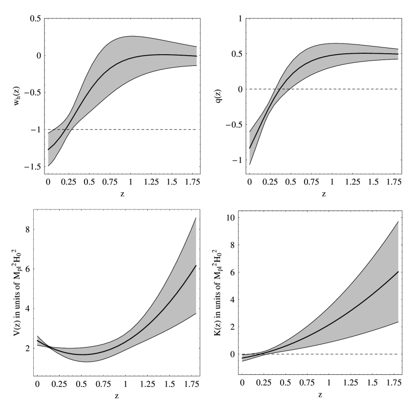
is used extensively (see r60 for instance). For Ansatz I with the prior , by using Eqs. (22), (24)–(26), (37), (40) and the corresponding best fit values of and , we can reconstruct the EoS of hessence , deceleration parameter , the potential of hessence , and the kinetic energy term of hessence as functions of the redshift , with the corresponding errors. We show the results in Fig. 3. It is easy to see that crossed and the universe transited from deceleration () to acceleration (); the reconstructed is well consistent with the three uncorrelated , and data points with their corresponding error bars for the weak prior r7 which are model-independent.
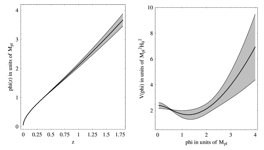
However, the error propagation equation (40) is invalid when we reconstruct the and hence the , since is obtained from a differential equation, i.e. Eq. (23). To evaluate the error propagations, we use the Monte Carlo method instead. That is, we generate a multivariate Gaussian distribution from the best fit parameters and the corresponding covariance matrix. And then, we randomly sample pairs of the parameters from this distribution. For each pair of , we can find the corresponding and from Eqs. (23) and (22) respectively. Hence, the is in hand. Finally, we can determine the mean and the corresponding error for the and from these samples, respectively. In Fig. 4, we show the reconstructed and with the corresponding errors for Ansatz I with the prior . In which, we have used the demonstrative initial value at and , and have chosen the solution with for the reconstructed ; we have done samplings.
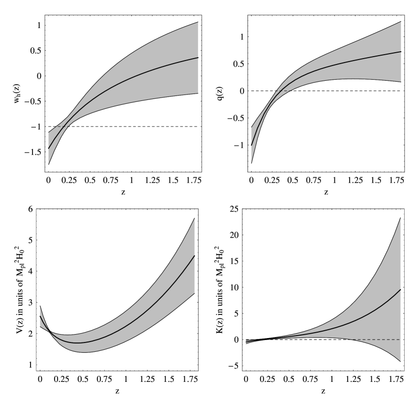
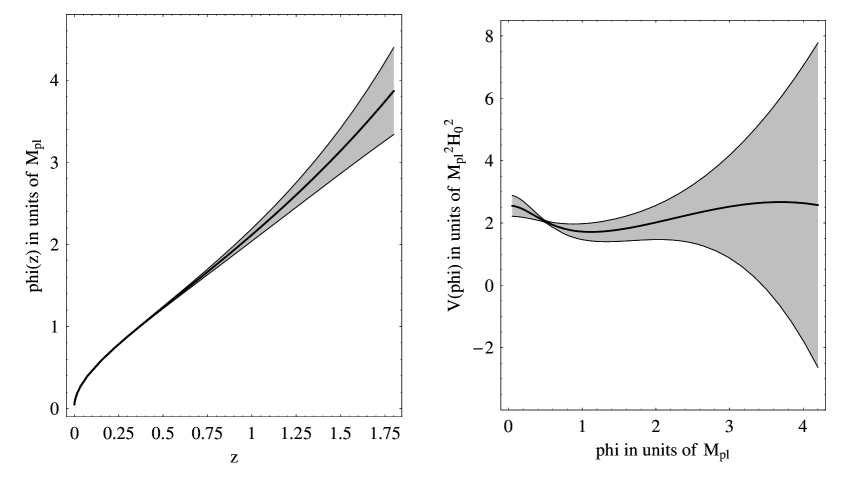
For Ansatz II, the method to reconstruct the EoS of hessence , deceleration parameter , the kinetic energy term of hessence , the potential of hessence , the as functions of the redshift , and the potential of hessence as function of , namely , is the same for Ansatz I. We present the results in Figs. 5 and 6. Once again, it is easy to see that crossed and the universe transited from deceleration () to acceleration (); the reconstructed is well consistent with the three uncorrelated , and data points with their corresponding error bars for the weak prior r7 which are model-independent.
V Discussion
In this work, we have developed a simple method based on the Hubble parameter to reconstruct the hessence dark energy. If the observational is obtained, the reconstruction of hessence dark energy is ready. It is worth noting that the reconstruction method presented here is sufficiently versatile for any .
As examples, we reconstructed the hessence dark energy with two familiar parameterizations for . It is easy to see that this reconstruction method works well. However, these parameterizations for are not the direct measure of from observational data. We can just say that they are consistent with the recent observational data. Can we be in a more comfortable situation? In fact, some efforts are aiming to a direct measure of from observational data. Analogous to the estimates of r8 , a method to obtaining the estimates of is proposed in r11 (see also r49 ). Actually, in the latest paper r7 by the Supernova Search Team led by Riess, a rough estimate of is obtained by using the new Hubble Space Telescope discoveries of SNe Ia at . Other new method to determine the Hubble parameter as function of redshift, , is also proposed in r50 recently. In a very different way, by using the differential ages of passively evolving galaxies determined from the Gemini Deep Deep Survey (GDDS) r51 and archival data r52 , Simon et al. determined in the range r53 ; r54 ; r55 ; r56 ; r57 ; r63 . However, up to now, all observational obtained by various methods are too rough to give a reliable reconstruction of hessence dark energy. A good news from r55 is that a large amount of data is expected to become available in the next few years. These include data from the AGN and Galaxy Survey (AGES) and the Atacama Cosmology Telescope (ACT), and by 2009 an order of magnitude increase in data is anticipated. Therefore, we are optimistic to the feasibility of the reconstruction method of hessence dark energy proposed in this work.
ACKNOWLEDGMENTS
We are grateful to Professor Rong-Gen Cai for helpful discussions. We also thank Zong-Kuan Guo, Xin Zhang, Hui Li, Meng Su, and Nan Liang, Rong-Jia Yang, Wei-Ke Xiao, Jian Wang, Yuan Liu, Wei-Ming Zhang, Fu-Yan Bian for kind help and discussions. We acknowledge partial funding support by the Ministry of Education of China, Directional Research Project of the Chinese Academy of Sciences and by the National Natural Science Foundation of China under project No. 10521001.
References
-
(1)
P. J. E. Peebles and B. Ratra,
Rev. Mod. Phys. 75, 559 (2003) [astro-ph/0207347];
T. Padmanabhan, Phys. Rept. 380, 235 (2003) [hep-th/0212290];
S. M. Carroll, astro-ph/0310342;
R. Bean, S. Carroll and M. Trodden, astro-ph/0510059;
V. Sahni and A. A. Starobinsky, Int. J. Mod. Phys. D 9, 373 (2000) [astro-ph/9904398];
S. M. Carroll, Living Rev. Rel. 4, 1 (2001) [astro-ph/0004075];
T. Padmanabhan, Curr. Sci. 88, 1057 (2005) [astro-ph/0411044];
S. Weinberg, Rev. Mod. Phys. 61, 1 (1989);
S. Nobbenhuis, Found. Phys. 36, 613 (2006) [gr-qc/0411093];
E. J. Copeland, M. Sami and S. Tsujikawa, hep-th/0603057;
R. Trotta and R. Bower, astro-ph/0607066. -
(2)
A. G. Riess et al. [Supernova Search Team Collaboration],
Astron. J. 116, 1009 (1998) [astro-ph/9805201];
S. Perlmutter et al. [Supernova Cosmology Project Collaboration], Astrophys. J. 517, 565 (1999) [astro-ph/9812133];
J. L. Tonry et al. [Supernova Search Team Collaboration], Astrophys. J. 594, 1 (2003) [astro-ph/0305008];
R. A. Knop et al., [Supernova Cosmology Project Collaboration], Astrophys. J. 598, 102 (2003) [astro-ph/0309368];
A. G. Riess et al. [Supernova Search Team Collaboration], Astrophys. J. 607, 665 (2004) [astro-ph/0402512]. -
(3)
P. Astier et al. [SNLS Collaboration],
Astron. Astrophys. 447, 31 (2006) [astro-ph/0510447];
J. D. Neill et al. [SNLS Collaboration], astro-ph/0605148. -
(4)
C. L. Bennett et al. [WMAP Collaboration],
Astrophys. J. Suppl. 148, 1 (2003) [astro-ph/0302207];
D. N. Spergel et al. [WMAP Collaboration], Astrophys. J. Suppl. 148 175 (2003) [astro-ph/0302209];
D. N. Spergel et al. [WMAP Collaboration], astro-ph/0603449;
L. Page et al. [WMAP Collaboration], astro-ph/0603450;
G. Hinshaw et al. [WMAP Collaboration], astro-ph/0603451;
N. Jarosik et al. [WMAP Collaboration], astro-ph/0603452. -
(5)
M. Tegmark et al. [SDSS Collaboration],
Phys. Rev. D 69, 103501 (2004) [astro-ph/0310723];
M. Tegmark et al. [SDSS Collaboration], Astrophys. J. 606, 702 (2004) [astro-ph/0310725];
U. Seljak et al., Phys. Rev. D 71, 103515 (2005) [astro-ph/0407372];
J. K. Adelman-McCarthy et al. [SDSS Collaboration], Astrophys. J. Suppl. 162, 38 (2006) [astro-ph/0507711];
K. Abazajian et al. [SDSS Collaboration], astro-ph/0410239; astro-ph/0403325; astro-ph/0305492;
M. Tegmark et al. [SDSS Collaboration], astro-ph/0608632. - (6) S. W. Allen, R. W. Schmidt, H. Ebeling, A. C. Fabian and L. van Speybroeck, Mon. Not. Roy. Astron. Soc. 353, 457 (2004) [astro-ph/0405340].
-
(7)
A. G. Riess et al. [Supernova Search Team Collaboration],
astro-ph/0611572.
The numerical data of the full sample are available at
http:braeburn.pha.jhu.edu/∼ariess/R06 or upon request to ariess@stsci.edu - (8) D. Huterer and A. Cooray, Phys. Rev. D 71, 023506 (2005) [astro-ph/0404062].
- (9) B. Feng, X. L. Wang and X. M. Zhang, Phys. Lett. B 607, 35 (2005) [astro-ph/0404224].
-
(10)
J. Q. Xia, G. B. Zhao, B. Feng, H. Li and X. M. Zhang,
Phys. Rev. D 73, 063521 (2006) [astro-ph/0511625];
J. Q. Xia, G. B. Zhao, B. Feng and X. M. Zhang, JCAP 0609, 015 (2006) [astro-ph/0603393];
G. B. Zhao, J. Q. Xia, B. Feng and X. M. Zhang, astro-ph/0603621;
J. Q. Xia, G. B. Zhao, H. Li, B. Feng and X. M. Zhang, Phys. Rev. D 74, 083521 (2006) [astro-ph/0605366];
J. Q. Xia, G. B. Zhao and X. M. Zhang, astro-ph/0609463;
G. B. Zhao, J. Q. Xia, H. Li, C. Tao, J. M. Virey, Z. H. Zhu and X. M. Zhang, astro-ph/0612728. - (11) Y. Wang and M. Tegmark, Phys. Rev. D 71, 103513 (2005) [astro-ph/0501351].
- (12) U. Alam, V. Sahni and A. A. Starobinsky, JCAP 0406, 008 (2004) [astro-ph/0403687].
-
(13)
B. A. Bassett, P. S. Corasaniti and M. Kunz,
Astrophys. J. 617, L1 (2004) [astro-ph/0407364];
A. Cabre, E. Gaztanaga, M. Manera, P. Fosalba and F. Castander, Mon. Not. Roy. Astron. Soc. Lett. 372, L23 (2006) [astro-ph/0603690]. - (14) S. Nesseris and L. Perivolaropoulos, Phys. Rev. D 70, 043531 (2004) [astro-ph/0401556].
- (15) R. Lazkoz, S. Nesseris and L. Perivolaropoulos, JCAP 0511, 010 (2005) [astro-ph/0503230].
- (16) Y. Wang and P. Mukherjee, Astrophys. J. 650, 1 (2006) [astro-ph/0604051].
- (17) A. Upadhye, M. Ishak and P. J. Steinhardt, Phys. Rev. D 72, 063501 (2005) [astro-ph/0411803].
- (18) H. Wei, R. G. Cai and D. F. Zeng, Class. Quant. Grav. 22, 3189 (2005) [hep-th/0501160].
- (19) H. Wei and R. G. Cai, Phys. Rev. D 72, 123507 (2005) [astro-ph/0509328].
- (20) M. Alimohammadi and H. Mohseni Sadjadi, Phys. Rev. D 73, 083527 (2006) [hep-th/0602268].
- (21) W. Zhao and Y. Zhang, Phys. Rev. D 73, 123509 (2006) [astro-ph/0604460].
- (22) H. Wei and R. G. Cai, Phys. Rev. D 73, 083002 (2006) [astro-ph/0603052].
- (23) Z. K. Guo, Y. S. Piao, X. M. Zhang and Y. Z. Zhang, Phys. Lett. B 608, 177 (2005) [astro-ph/0410654].
- (24) X. F. Zhang, H. Li, Y. S. Piao and X. M. Zhang, Mod. Phys. Lett. A 21, 231 (2006) [astro-ph/0501652].
-
(25)
H. Wei and R. G. Cai,
Phys. Lett. B 634, 9 (2006) [astro-ph/0512018].
Z. K. Guo, Y. S. Piao, X. M. Zhang and Y. Z. Zhang, astro-ph/0608165;
X. Zhang and F. Q. Wu, Phys. Rev. D 72, 043524 (2005) [astro-ph/0506310];
X. Zhang, Int. J. Mod. Phys. D 14, 1597 (2005) [astro-ph/0504586];
Y. F. Cai, H. Li, Y. S. Piao and X. M. Zhang, gr-qc/0609039;
Y. F. Cai, M. Z. Li, J. X. Lu, Y. S. Piao, T. T. Qiu and X. M. Zhang, hep-th/0701016. -
(26)
M. Z. Li, B. Feng and X. M. Zhang,
JCAP 0512, 002 (2005) [hep-ph/0503268];
X. F. Zhang and T. T. Qiu, astro-ph/0603824;
Z. Chang, F. Q. Wu and X. Zhang, Phys. Lett. B 633, 14 (2006) [astro-ph/0509531];
H. S. Zhang and Z. H. Zhu, Phys. Rev. D 73, 043518 (2006) [astro-ph/0509895];
H. S. Zhang and Z. H. Zhu, astro-ph/0611834. - (27) H. Wei and R. G. Cai, astro-ph/0607064.
- (28) A. Vikman, Phys. Rev. D 71, 023515 (2005) [astro-ph/0407107].
- (29) G. B. Zhao, J. Q. Xia, M. Li, B. Feng and X. M. Zhang, Phys. Rev. D 72, 123515 (2005) [astro-ph/0507482].
- (30) M. Kunz and D. Sapone, astro-ph/0609040.
-
(31)
K. Kadota, S. Dodelson, W. Hu and E. D. Stewart,
Phys. Rev. D 72, 023510 (2005) [astro-ph/0505158];
A. R. Liddle and A. N. Taylor, Phys. Rev. D 65, 041301 (2002) [astro-ph/0109412];
L. C. Garcia de Andrade, Mod. Phys. Lett. A 16, 1353 (2001);
I. J. Grivell and A. R. Liddle, Phys. Rev. D 61, 081301 (2000) [astro-ph/9906327];
E. J. Copeland, I. J. Grivell, E. W. Kolb and A. R. Liddle, Phys. Rev. D 58, 043002 (1998) [astro-ph/9802209];
G. Mangano, G. Miele and C. Stornaiolo, Mod. Phys. Lett. A 10, 1977 (1995) [astro-ph/9507117];
E. J. Copeland, E. W. Kolb, A. R. Liddle and J. E. Lidsey, Phys. Rev. D 49, 1840 (1994) [astro-ph/9308044]. - (32) Z. K. Guo, N. Ohta and Y. Z. Zhang, Phys. Rev. D 72, 023504 (2005) [astro-ph/0505253].
- (33) Z. K. Guo, N. Ohta and Y. Z. Zhang, astro-ph/0603109.
- (34) M. Sahlen, A. R. Liddle and D. Parkinson, astro-ph/0610812.
- (35) C. Li, D. E. Holz and A. Cooray, astro-ph/0611093.
- (36) W. Zhao, astro-ph/0604459.
- (37) S. Fay and R. Tavakol, Phys. Rev. D 74, 083513 (2006) [astro-ph/0606431].
- (38) S. Rahvar and M. S. Movahed, astro-ph/0604206.
- (39) M. Sahlen, A. R. Liddle and D. Parkinson, Phys. Rev. D 72, 083511 (2005) [astro-ph/0506696].
- (40) A. Shafieloo, U. Alam, V. Sahni and A. A. Starobinsky, Mon. Not. Roy. Astron. Soc. 366, 1081 (2006) [astro-ph/0505329].
- (41) A. A. Sen, JCAP 0603, 010 (2006) [astro-ph/0512406].
- (42) H. Li, Z. K. Guo and Y. Z. Zhang, Mod. Phys. Lett. A 21, 1683 (2006) [astro-ph/0601007].
- (43) S. Tsujikawa, Phys. Rev. D 72, 083512 (2005) [astro-ph/0508542].
-
(44)
X. Zhang, astro-ph/0604484;
X. Zhang, Phys. Rev. D 74, 103505 (2006) [astro-ph/0609699];
J. F. Zhang, X. Zhang and H. Y. Liu, astro-ph/0612642. -
(45)
L. Xu, H. Liu and Y. Ping,
Int. J. Theor. Phys. 45, 843 (2006) [astro-ph/0601471];
L. Xu, H. Liu and C. Zhang, Int. J. Mod. Phys. D 15, 215 (2006) [astro-ph/0510673]. - (46) V. Sahni and A. Starobinsky, astro-ph/0610026.
- (47) U. Alam, V. Sahni, T. D. Saini and A. A. Starobinsky, Mon. Not. Roy. Astron. Soc. 354, 275 (2004) [astro-ph/0311364].
- (48) A. A. Sen and R. J. Scherrer, Phys. Rev. D 72, 063511 (2005) [astro-ph/0507717].
- (49) R. A. Daly and S. G. Djorgovski, Astrophys. J. 612, 652 (2004) [astro-ph/0403664].
- (50) C. Bonvin, R. Durrer and M. Kunz, Phys. Rev. Lett. 96, 191302 (2006) [astro-ph/0603240].
- (51) R. G. Abraham et al. [GDDS Collaboration], Astron. J. 127, 2455 (2004) [astro-ph/0402436].
-
(52)
T. Treu, M. Stiavelli, S. Casertano, P. Moller and G. Bertin,
Mon. Not. Roy. Astron. Soc. 308, 1037 (1999);
T. Treu, M. Stiavelli, P. Moller, S. Casertano and G. Bertin, Mon. Not. Roy. Astron. Soc. 326, 221 (2001) [astro-ph/0104177];
T. Treu, M. Stiavelli, S. Casertano, P. Moller and G. Bertin, Astrophys. J. Lett. 564, L13 (2002);
J. Dunlop, J. Peacock, H. Spinrad, A. Dey, R. Jimenez, D. Stern and R. Windhorst, Nature 381, 581 (1996);
H. Spinrad, A. Dey, D. Stern, J. Dunlop, J. Peacock, R. Jimenez and R. Windhorst, Astrophys. J. 484, 581 (1997);
L. A. Nolan, J. S. Dunlop, R. Jimenez and A. F. Heavens, Mon. Not. Roy. Astron. Soc. 341, 464 (2003) [astro-ph/0103450]. - (53) R. Jimenez, L. Verde, T. Treu and D. Stern, Astrophys. J. 593, 622 (2003) [astro-ph/0302560].
- (54) J. Simon, L. Verde and R. Jimenez, Phys. Rev. D 71, 123001 (2005) [astro-ph/0412269].
- (55) L. Samushia and B. Ratra, Astrophys. J. 650, L5 (2006) [astro-ph/0607301].
- (56) Z. L. Yi and T. J. Zhang, astro-ph/0605596, MPLA in press.
- (57) H. Wei and S. N. Zhang, Phys. Lett. B 644, 7 (2007) [astro-ph/0609597].
- (58) S. Nesseris and L. Perivolaropoulos, Phys. Rev. D 72, 123519 (2005) [astro-ph/0511040].
- (59) L. Perivolaropoulos, Phys. Rev. D 71, 063503 (2005) [astro-ph/0412308].
- (60) U. Alam, V. Sahni, T. D. Saini and A. A. Starobinsky, astro-ph/0406672.
- (61) S. Nesseris and L. Perivolaropoulos, astro-ph/0610092.
- (62) Y. G. Gong and A. Z. Wang, astro-ph/0612196.
- (63) P. X. Wu and H. W. Yu, gr-qc/0612055.
- (64) E. Di Pietro and J. F. Claeskens, Mon. Not. Roy. Astron. Soc. 341, 1299 (2003) [astro-ph/0207332].
- (65) P. S. Apostolopoulos and N. Tetradis, Phys. Rev. D 74, 064021 (2006) [hep-th/0604014].
-
(66)
E. Elizalde, S. Nojiri and S. D. Odintsov,
Phys. Rev. D 70, 043539 (2004) [hep-th/0405034];
S. Nojiri, S. D. Odintsov and S. Tsujikawa, Phys. Rev. D 71, 063004 (2005) [hep-th/0501025];
S. Nojiri and S. D. Odintsov, Gen. Rel. Grav. 38, 1285 (2006) [hep-th/0506212];
S. Capozziello, S. Nojiri and S. D. Odintsov, Phys. Lett. B 632, 597 (2006) [hep-th/0507182];
S. Nojiri and S. D. Odintsov, Phys. Rev. D 72, 023003 (2005) [hep-th/0505215];
E. Elizalde, S. Nojiri, S. D. Odintsov and P. Wang, Phys. Rev. D 71, 103504 (2005) [hep-th/0502082]. -
(67)
E. O. Kahya and V. K. Onemli, gr-qc/0612026;
T. Brunier, V. K. Onemli and R. P. Woodard, Class. Quant. Grav. 22, 59 (2005) [gr-qc/0408080]. - (68) U. Alam, V. Sahni and A. A. Starobinsky, astro-ph/0612381.
-
(69)
P. T. Silva and O. Bertolami,
Astrophys. J. 599, 829 (2003) [astro-ph/0303353];
O. Bertolami, A. A. Sen, S. Sen and P. T. Silva, Mon. Not. Roy. Astron. Soc. 353, 329 (2004) [astro-ph/0402387];
M. C. Bento, O. Bertolami, N. M. C. Santos and A. A. Sen, Phys. Rev. D 71, 063501 (2005) [astro-ph/0412638]. - (70) V. Barger, Y. Gao and D. Marfatia, astro-ph/0611775.
-
(71)
W. M. Wood-Vasey et al. [ESSENCE Collaboration],
astro-ph/0701041;
G. Miknaitis et al. [ESSENCE Collaboration], astro-ph/0701043. - (72) The WMAP first year data (WMAP1) suggest that . Combining the WMAP three year data (WMAP3) with the SNe Gold data, it is found that , while for combining WMAP3 data with the CFHTLS lensing data. See Ref. r4 for details. On the other hand, the SDSS data suggest that (see the third one in Ref. r5 ). The SNLS data r3 suggest that . The ESSENCE data r71 give also. So, as in many works in the literature, we consider the prior throughout this paper.