The Hanle Effect in Atomic and Molecular Lines:
A New Look at the Sun’s Hidden Magnetism

Abstract

This paper reviews some of the most recent advances in the application of the Hanle effect to solar physics, and how these developments are allowing us to explore the magnetism of the photospheric regions that look “empty” in solar magnetograms—that is, the Sun’s “hidden” magnetism. In particular, we show how a joint analysis of the Hanle effect in atomic and molecular lines indicates that there is a vast amount of hidden magnetic energy and unsigned magnetic flux localized in the (intergranular) downflowing regions of the quiet solar photosphere, carried mainly by tangled fields at sub-resolution scales with strengths between the equipartition field values and $\sim 1$ kG.

¹Instituto de Astrofísica de Canarias, Vía Láctea s/n, E-38205 La Laguna, Tenerife, Spain
²Consejo Superior de Investigaciones Científicas, Spain
³Main Astronomical Observatory, National Academy of Sciences, Zabolotnogo 27, 03680 Kyiv, Ukraine

1. Introduction

At any given time during the solar magnetic activity cycle most of the solar surface is covered by the internetwork regions of the “quiet” Sun. Although such regions look “empty” (i.e., devoided of magnetic signatures) in low-resolution magnetograms, high-spatial-resolution observations reveal the presence of mixed magnetic polarities with a mean unsigned flux density of the order of 10 G, when choosing the best compromise between the polarimetric sensitivity and the spatio-temporal resolution currently attainable (e.g., Lin & Rimmele 1999; Domínguez Cerdeña, Kneer, & Sánchez Almeida 2003; Khomenko et al. 2003; Lites & Socas-Navarro 2004; Martínez González, Collados, & Ruiz Cobo 2006). However, when these Zeeman-effect polarization signals are interpreted considering that the magnetic field is not spatially resolved (for example, by assuming that one or more magnetic components coexist with a non-magnetic component within the spatio-temporal resolution element of the observations), it is found that the filling factor of the magnetic component(s) is $\sim 1$%.

The disadvantage of the Zeeman effect as a diagnostic tool is that the amplitudes of the measured polarization signals become smaller with the increasing degree of cancellation of mixed magnetic polarities within the spatio-temporal resolution element. Therefore, vanishing Zeeman polarization does not necessarily imply absence of magnetic fields. On the contrary, the photospheric plasma of the quiet Sun is expected to be permeated by highly tangled field lines with resulting mixed magnetic polarities on very small spatial scales, well beyond the current spatial resolution limit (e.g., Stenflo 1994; Cattaneo 1999; Sánchez Almeida, Emonet, & Cattaneo 2003a; Stein & Nordlund 2003). For this reason, it is believed that Zeeman-effect diagnostics with the present-day instrumentation is showing us only the “tip of the iceberg” of solar surface magnetism ($\sim 1$% of the photospheric volume).

How can we reliably investigate the magnetism of the remaining $\sim 99$% of the quiet solar atmosphere? How can we obtain empirical information on the distribution of mixed-polarity magnetic fields at sub-resolution scales that are “hidden” to the Zeeman effect? Do such fields carry most of the unsigned magnetic flux and magnetic energy of the Sun, or is this flux and/or the magnetic energy dominated by small-scale magnetic flux concentrations in the kG range, as some recent investigations based on the Zeeman effect of the Fe i lines at 6301.5 Å and 6302.5 Å seem to suggest? How is the magnetic energy of the quiet Sun distributed between upflows and downflows? Is the total magnetic energy stored in the quiet internetwork regions greater or smaller than that of the kG fields of the super-granulation network? Is this energy significant enough to compensate for the radiative losses of the outer solar atmosphere? How is energy transported and dissipated in a mixed magnetic-polarity environment? Does this hidden magnetic flux complicate the topology of the magnetic fields of the outer solar atmosphere, or there simply are magnetic canopies, with mainly horizontal fields, in the quiet regions of the solar chromosphere?

Since the Zeeman effect as a diagnostic tool is “blind” to magnetic fields that are tangled on scales too small to be resolved, the investigation of the magnetism of the quiet Sun via spectro-polarimetry must rely on other tools as well. In addition to Zeeman diagnostics developed to interpret the observed asymmetries of Stokes profiles—resulting from the co-existence of opposite magnetic polarities that do not cancel completely within the resolution element (e.g., Sánchez Almeida et al. 1996; Socas-Navarro & Sánchez Almeida 2002), and/or from hyperfine-structure effects (e.g., López Ariste, Tomczyk, & Casini 2002), we also need to apply “new” diagnostic techniques based on physical mechanisms whose observable signatures do not suffer from cancellation effects.

Two such mechanisms are the Hanle effect and the line broadening by the Zeeman effect (e.g., Stenflo 1994). We argue that the Hanle effect can be suitably complemented with the Zeeman broadening of the intensity profiles of some carefully selected near-IR lines, as a tool to obtain information on the distribution of tangled magnetic fields at sub-resolution scales in the quiet regions of the solar photosphere. In particular, we will review in some detail how the most recent advances in the application of the Hanle effect to solar physics has led us to the conclusion that the hidden magnetic fields of the quiet Sun carry a vast amount of unsigned flux and energy.

In Sect. 2 we highlight some of the most recent investigations on the magnetism of the quiet Sun based on the interpretation of Zeeman polarization signals. In Sect. 3 we consider the Hanle effect in the Sr i 4607 Å line, showing how the observed scattering polarization amplitudes suggest the presence of a tangled magnetic field at sub-resolution scales, with a mean field strength $\langle B\rangle\sim 100$ G. In Sect. 4 we address the question of whether a significantly smaller $\langle B\rangle$ could perhaps be inferred by assuming a magnetic field topology different from that of an isotropic microturbulent field. In Sect. 5 we discuss the direct observational evidence of magnetic depolarization provided by other spectral lines, such as the multiplet No. 42 of Ti i. In Sect.  6 we review the work done on the Hanle effect in molecular lines, pointing out some key questions (e.g., the fact that the inferred $\langle B\rangle\sim 10$ G), whose answer led us to the conclusion that the strength of the hidden field “fluctuates” on the spatial scales of solar granulation, with rather weak fields above the granular regions, but with a distribution of stronger fields in the intergranular regions (capable of producing saturation of the Hanle effect in the Sr i 4607 Å line formed there). Finally, in Sect. 7 we summarize the main conclusions and discuss possible lines of future research.

2. Diagnostics of Zeeman-Effect Polarization

Over the last few years the observational and theoretical evidence of small-scale mixtures of weak and strong fields in the quiet Sun has increased considerably (e.g., Lin & Rimmele 1999; Sánchez Almeida & Lites 2000; Lites 2002; Socas-Navarro & Sánchez Almeida 2003; Khomenko et al. 2003; Socas-Navarro & Lites 2004; Sánchez Almeida et al. 2003a; Sánchez Almeida, Domínguez Cerdeña, & Kneer 2003b; Cattaneo 1999; Stein & Nordlund 2003; Vögler 2003), but so has the controversy about the true abundance of kG fields in the internetwork regions of the quiet Sun (e.g., Domínguez Cerdeña et al. 2003; Bellot Rubio & Collados 2003; Lites & Socas-Navarro 2004; Socas-Navarro, Martínez Pillet, & Lites 2004; Sánchez Almeida et al. 2003b, 2004; de Wijn et al. 2005; Khomenko et al. 2005; Martínez Gonzalez et al. 2006; Collados, this conference). For example, Domínguez Cerdeña et al. (2003) interpret the systematic difference between the flux densities measured in the Fe i 6301.5/6302.5 Å lines as evidence for small-scale magnetic structures with intrinsic field strengths larger than 1 kG, occupying 2% of the solar surface. This would imply an abundance of kG fields in the internetwork regions of the Sun significantly larger than that inferred by Khomenko et al. (2003) from measurements of the Stokes profiles in the Fe i lines at 15648 Å and 15652 Å.

Concerning proxy magnetometry, it is important to mention that de Wijn et al. (2005) measured a surface density of internetwork bright points (IBP) of 0.02 Mm^-2 in sharp G-band images obtained with the Dutch Open Telescope, and concluded that the observed IBPs seem to outline mesogranular cell-like structures. Sánchez Almeida et al. (2004) reported instead that in their best G-band image (which contained a small network patch) obtained with the 1-m Swedish Solar Telescope, the density of bright points is 0.3 Mm^-2, which led them to conclude that detected bright points cover 0.7% of the solar surface.

Recently, Khomenko (2006) has suggested that the application of Stenflo’s (1973) line-ratio technique to the observed Stokes-$V$ profiles produced by the Zeeman effect in the Fe i 6301.5/6302.5 Å lines could overestimate the fraction of (internetwork) quiet Sun occupied by field strengths $B>1$ kG (see also Figs. 1 and 2 in Khomenko & Collados 2006), because these lines do not have exactly the same absorption coefficient or the same behavior in the dynamic and highly inhomogenous solar atmosphere (Shchukina & Trujillo Bueno 2001). This fact is illustrated in the left panels of Fig. 1, which shows results of three-dimensional (3D), non-LTE radiative transfer calculations. Interestingly, the right panels of Fig. 1 suggest that the application of the line-ratio technique to the Fe i 15648/15652 Å lines could indeed be a reliable strategy. A similar calculation for the Fe i 5250.21/5247.05 Å lines reveals a behavior for $H_{\rm VIS}$(red) and $H_{\rm VIS}$(blue) (with $\Delta\lambda=\pm 30$ mÅ) more or less similar to that shown in the left panels of Fig. 1, but with $H_{\rm VIS}^{5250}-H_{\rm VIS}^{5247}\approx 0$ km. It is also important to note that while $S_{\rm line}\approx B_{\nu}$ for the 5250.21/5247.05 Å lines, $(S_{\rm line}/B_{\nu})_{6301.5}<(S_{\rm line}/B_{\nu})_{6302.5}<1$ (see Fig. 8 of Shchukina & Trujillo Bueno 2001, right panel).

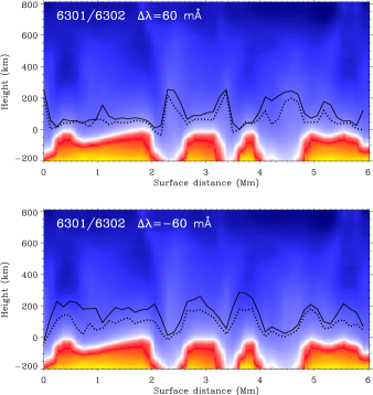
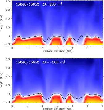
Figure 1.: Plots of the horizontal fluctuation of the height $H_{\rm line}$ at which $\tau_{\rm line}(\Delta\lambda)=1$, for different lines and values of $\Delta\lambda$, in a simulated observation at disk-center using a realistic 3D hydrodynamical model of the solar photosphere. The adopted values for $\Delta\lambda$ are typical distances from line center at which internetwork Stokes-$V$ profiles of the selected lines have their “red” and “blue” lobes. Left: Fe i 6301.5 Å (solid line) and 6302.5 Å (dotted line), for $\Delta\lambda=+60$ mÅ (top panel) and $\Delta\lambda=-60$ mÅ (bottom panel). Note that $H_{\rm VIS}^{6301.5}-H_{\rm VIS}^{6302.5}\approx 100$ km, which is a significant height difference. Note also that in the (intergranular) downflowing regions $H_{\rm VIS}({\rm blue})\ll H_{\rm VIS}({\rm red})$, while in the (granular) upflowing regions $H_{\rm VIS}({\rm blue})\gg H_{\rm VIS}({\rm red})$. Right: Fe i 15648 Å (solid line) and 15652 Å(dotted line), for $\Delta\lambda=+200$ mÅ (top panel) and $\Delta\lambda=-200$ mÅ (bottom panel). Note that $H_{\rm IR}^{15648}-H_{\rm IR}^{15652}\approx 0$ km, and that $H_{\rm IR}({\rm blue})\approx H_{\rm IR}({\rm red})$ in the granular and intergranular regions, independently. Finally, it is also important to note that $H_{\rm VIS}>H_{\rm IR}$.

Therefore, it is at present unclear whether or not the small-scale magnetic fields that we “see” in the internetwork regions of the Sun via the longitudinal Zeeman effect in the 6301.5/6302.5 Å lines (whose filling factor is $\sim 1$%) are sufficiently strong to carry a truly significant fraction of the unsigned magnetic flux and magnetic energy of the Sun. In this respect, we note that Keller et al. (1994) already applied Stenflo’s (1973) magnetic line-ratio technique to measurements of the Stokes-$V$ profiles of the Fe i 5250.21/5247.05 Å lines, and concluded that the strength of solar internetwork fields at the height of line formation is below 1 kG with a high probability. Obviously, multiline observations with high spatial resolution and polarimetric sensitivity are urgently needed.

3. The Hanle Effect in the Sr i 4607 Å Line

An unresolved, tangled magnetic field tends to reduce the line scattering polarization amplitudes with respect to the zero magnetic field case. This so-called Hanle effect has the required diagnostic potential for investigating tangled magnetic fields at sub-resolution scales (Stenflo 1982). The critical magnetic field strength (measured in G) that is sufficient to produce (via the upper-level Hanle effect) a significant change in the line’s scattering polarization amplitude, when the excitation of the atomic or molecular system is dominated by radiative transition, is (e.g., Trujillo Bueno 2001)

$$B_{\rm H}={\frac{1.137\times 10^{-7}}{t_{\rm life}\,g}}\,,$$ (1)

where $g$ and $t_{\rm life}$ are, respectively, the Landé factor and the radiative lifetime (measured in seconds) of the upper level of the spectral line under consideration (e.g., $B_{\rm H}\approx 23$ G for the Sr i 4607 Å line).

The main problem with choosing the Hanle effect as a diagnostic tool of the quiet Sun magnetism is how to apply it to obtain reliable information, given that it relies on a comparison between the observed linear polarization and that calculated for the zero-field reference case. Shchukina & Trujillo Bueno (2003) have shown that the particular one-dimensional (1D) approach applied by Faurobert-Scholl et al. (1995) and Faurobert et al. (2001) to the scattering polarization observed in the Sr i 4607 Å line yields artificially low values for the strength of the hidden field—that is, $\langle B\rangle\approx 20$ G, as shown by the dashed line in the left panel of Fig. 3 in Shchukina & Trujillo Bueno (2003). This is because the scattering polarization amplitudes calculated by Faurobert-Scholl et al. (1995) and Faurobert et al. (2001) for the zero-field reference case, $(Q/I)_{B=0}$, was seriously underestimated due to their choice of the free parameters of “classical” stellar spectroscopy (that is, micro- and macro-turbulence for line broadening), which led to a sizable error in the value of the Hanle depolarization factor ${\cal D}=(Q/I)/(Q/I)_{B=0}$, where $Q/I$ is the observed polarization amplitude.

Note that for the currently used model of a microturbulent field, the depolarization factor ${\cal D}$ is similar to the factor ${\cal H}^{(2)}$ given by Eq. (A-16) of Trujillo Bueno & Manso Sainz (1999), with ${\cal H}^{(2)}=1$ for $B=0$ G and ${\cal H}^{(2)}=1/5$ for $B>B_{\rm satur}$ (where $B_{\rm satur}\sim 10\,B_{\rm H}$ is the saturation field of the Hanle effect for the spectral line under consideration). To understand why ${\cal D}\approx{\cal H}^{(2)}$ it suffices to note that Eq. (4) of Trujillo Bueno (2003a) leads to the following Eddington-Barbier approximation for the emergent $Q/I$ at the line-core of the Sr i 4607 Å line,

$$Q/I\approx\frac{3}{2\sqrt{2}}(1-\mu^{2})\frac{{\cal H}^{(2)}}{1+{\delta}_{u}}\,{\cal A}\,,$$ (2)

where ${\mu}=\cos{\theta}$ (with $\theta$ the angle between the solar radius vector through the observed point and the line-of-sight), ${\delta}_{u}=D^{(2)}\,t_{\rm life}\approx D^{(2)}/A_{ul}$ is basically the upper-level rate of (depolarizing) elastic collisions in units of the Einstein $A_{ul}$ coefficient, and ${\cal A}=J^{2}_{0}/J^{0}_{0}$ is the degree of anisotropy of the spectral line radiation (e.g., Trujillo Bueno 2001). The particular 1D radiative transfer fitting approach of Faurobert-Scholl et al. (1995) and Faurobert et al. (2001) gives ${\cal D}\approx 0.8$ when using the accurate observational data shown in Fig. 2.

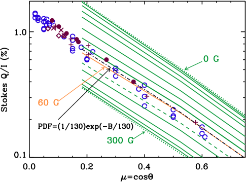
Figure 2.: Center-to-limb variation of the fractional linear polarization in the center of the Sr i 4607 Å line after subtraction of the continuum polarization. ($\circ$) various observations taken by Stenflo et al. (1997) during a minimum of the solar cycle. The remaining symbols correspond to observations taken during the most recent maximum of the solar cycle: ($\diamond$) observations obtained by Trujillo Bueno et al. (2001); ($\times$ and $+$) observations taken by Bommier & Molodij (2002) and by Bommier et al. (2005), respectively; ($\bullet$) observations obtained in collaboration with M. Bianda. Colored (or solid, dashed, and dotted) lines show the results of our 3D scattering polarization calculations in the presence of a volume-filling and single value microturbulent field (from top to bottom: 0, 5, 10, 15, 20, 30, 40, 50, 60, 80, 100, 150, 200, 250 and 300 G). Note that there is no evidence of a significant modulation of the observed $Q/I$ with the solar magnetic activity cycle, and that the best average fit to the observations is obtained for 60 G. The black, dashed-dotted line indicates the resulting $Q/I$ amplitudes for the case of a microturbulent field described by an exponential Probability Distribution Function with $\langle B\rangle=130$ G. (From Trujillo Bueno, Shchukina, & Asensio Ramos 2004.)

Trujillo Bueno, Shchukina, & Asensio Ramos (2004) pointed out that reliable Hanle-effect diagnostics can be achieved by means of 3D multilevel scattering polarization calculations in snapshots taken from realistic simulations of solar surface convection (see Asplund et al. 2000). These radiation hydrodynamical simulations of the photospheric physical conditions are very convincing because spectral synthesis of a multitude of iron lines shows remarkable agreement with the observed spectral line profiles (e.g., Shchukina & Trujillo Bueno 2001). Therefore, we have used snapshots taken from such time-dependent hydrodynamical simulations in order to calculate the emergent Stokes profiles via 3D scattering polarization calculations using realistic multilevel atomic models. Our first target was the Sr i line at 4607 Å, which is a normal triplet transition with $A_{ul}\approx 2\times 10^{8}\,{\rm s}^{-1}$ and Landé factor $g_{J_{u}}=1$. We point out that our synthetic intensity profiles (which take into account the Doppler shifts of the convective flow velocities in the 3D model) are in excellent agreement with the observations when the meteoritic strontium abundance is chosen. However, we find that the spatially and temporally averaged emergent Stokes profiles for $B=0$ G give a $Q/I$ that is substantially larger than observed, thus indicating the need for invoking magnetic depolarization. As can be easily deduced from Fig. 2, we obtain ${\cal D}\approx 0.4$.

If our 3D result for ${\cal D}$ is correct, then any analysis based on ${\cal H}^{(2)}\approx{\cal D}\approx 0.8$ (i.e., based on the ${\cal D}$ values obtained when the accurate $Q/I$ measurements of Fig. 2 are normalized to the $(Q/I)_{B=0}$ estimate of Faurobert and coworkers) would imply a mean strength of the hidden field substantially smaller than the actual value (e.g., the simplified analyses carried out by Sánchez Almeida et al. 2003a and Stenflo & Holzreuter 2003, which were based on the estimation of ${\cal D}$ that Faurobert-Scholl et al. 1995 obtained from older observations). Obviously, the only way to arrive at a solid conclusion concerning the unsigned magnetic flux and magnetic energy density carried by the hidden field is to use the correct value of the depolarization factor, ${\cal D}$.

We think that at present the 3D analysis of the observed scattering polarization in the Sr i 4607 Å line carried out by Trujillo Bueno et al. (2004) provides the most accurate estimation of ${\cal D}$, not only because of the fact already mentioned that our synthetic intensity profiles (which take into account the Doppler shifts of the convective flow velocities in the 3D model) are already in excellent agreement with the observed intensity profiles without having to use the free parameters of classical stellar spectroscopy, but also because we carefully computed the radiation field’s anisotropy in the 3D hydrodynamical model (e.g., Fig. 1 of Shchukina & Trujillo Bueno 2003). We solved the statistical equilibrium equations for the elements of the atomic density matrix and the Stokes-vector transfer equations using efficient radiative transfer methods (Trujillo Bueno 2003b), and adopting realistic collisional depolarizing rate values (Faurobert-Scholl et al. 1995), which turn out to be the largest rates among those found in the literature. It is also important to point out that the recent work of Bommier et al. (2005) strongly supports the result for ${\cal D}$ of Trujillo Bueno et al. (2004).

We may thus conclude that the depolarization required to fit the $Q/I$ observations of the Sr i 4607 Å line is with high probability of magnetic origin. For the moment we have assumed that the magnetic field is isotropic and microturbulent, which we consider as a reasonable approximation for estimating the mean strength of the “hidden” field. It is obvious that with a single spectral line we do not have enough information to constrain the shape of the Probability Distribution Function, ${\rm PDF}(B)$, describing the fraction of quiet Sun occupied by magnetic fields with strength $B$. For this reason, we chose the functional form of the PDF, like others have also done (e.g., Faurobert-Scholl et al. 1995; Faurobert et al. 2001; Bommier et al. 2005; Domínguez Cerdeña, Sánchez Almeida, & Kneer 2006). The key point, however, is to be conservative in the choice of the functional form of the PDF, in order to avoid exaggerating the resulting mean strength of the hidden field. For this reason, although we carried out calculations for several functional forms of the PDF, Trujillo Bueno et al. (2004) presented results only for the two forms: (a) ${\rm PDF}(B)={\delta}(B-\langle B\rangle)$ and (b) ${\rm PDF}(B)={\rm e}^{-B/\langle B\rangle}/\langle B\rangle$, where $\langle B\rangle$ is the mean field strength.

The idealized model corresponding to case (a) will clearly underestimate $\langle B\rangle$, but it is interesting to compare the ensuing magnetic energy with that corresponding to the kG fields of the network patches. The much more realistic case (b) is suggested by numerical experiments of turbulent dynamos and magnetoconvection (e.g., Cattaneo 1999; Stein & Nordlund 2003; Vögler 2003). The “surface” PDF in some of these numerical experiments tends to be instead a stretched exponential, which, to a first approximation, can be fitted by a Voigt function whose tail extends further out into the kG range than an exponential. Therefore, by choosing an exponential PDF instead of a Voigt PDF (or instead of any other better fitting function) we guarantee that we are not exaggerating our estimation of $\langle B\rangle$. For the more realistic case (b), we also found it important to compare the resulting magnetic energy with that corresponding to the kG fields of the network patches (Trujillo Bueno et al. 2004).

As shown in Fig. 2, for the standard case (a) of a single-value microturbulent field we found that $\langle B\rangle\approx 60$ G leads to a notable agreement with the observed $Q/I$. Note that the strength of the hidden field required to explain the $Q/I$ observations seems to decrease with height in the atmosphere, from the 70 G needed to explain the observations at $\mu=0.6$ to the 50 G required to fit the observations at $\mu=0.1$. This corresponds to an approximate height range between 200 and 400 km above the solar visible “surface”.

Concerning the case of an exponential PDF, we see in Fig. 2 that $\langle B\rangle\approx 130$ G yields a fairly good fit to the observed fractional linear polarization. In this more realistic case $E_{\rm m}={\langle B^{2}\rangle}/8{\pi}\approx 1300\,{\rm erg\,cm^{-3}}$ (i.e., $\langle B^{2}\rangle^{1/2}\approx 180$ G), which is about 20% of the kinetic energy density produced by convective motions at a height of 200 km in the 3D photospheric model. As pointed out by Trujillo Bueno et al. (2004), for this case the total magnetic energy stored in the internetwork regions turns out to be larger than that corresponding to the kG fields of the network patches.

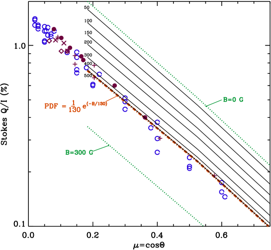
Figure 3.: This figure is similar to Fig. 2, with the black dashed-dotted line showing the same good overall fit obtained with an exponential PDF with $\langle B\rangle=130$ G. The two dotted lines labeled $B=0$ G and $B=300$ G are also identical to those of Fig. 2. In contrast, the solid-lines labeled by the values $B_{\rm final}=50,100,150,200,300,400,500$ G show the calculated $Q/I$ amplitudes imposing a cut-off of the exponential PDF at $B_{\rm final}$. This figure shows that, in order to be able to fit the $Q/I$ observations, we need to take into account all the magnetic fields with strengths between zero and 500 G, whose filling factor is 98%. The remaining magnetic fields of the exponential PDF above the cut-off of 500 G correspond to a filling factor of 2%, and they make no significant contribution to the Hanle depolarization.

Domínguez Cerdeña et al. (2006) have recently arrived at similar conclusions by combining magnetic field strength measurements based on the Zeeman effect in the Fe i lines at 6301.5 Å, 6302.5 Å, 15648 Å, and 15652 Å, and the Hanle effect in the Sr i 4607 Å line. They approximated the total PDF with $P(B)=w\,P_{\rm H}(B)+(1-w)\,P_{\rm Z}(B)$, where $P_{\rm Z}(B)$ is a PDF inferred from the Zeeman signals, $P_{\rm H}(B)$ a PDF that fits the Hanle signals, and $w\approx 1$. The fact that these authors arrive at conclusions similar to those of Trujillo Bueno et al. (2004), can be explained by noting that: 1) the fraction of quiet Sun producing the Zeeman polarization signals was only $\sim 1.5\%$; 2) they used our value for the depolarization factor of the Sr i 4607 Å line (${\cal D}=0.4$); and 3) they imposed the reasonable constraint that the magnetic energy density has to be significantly smaller than the kinetic energy density of the granular motions. What makes their work different from ours is that their $P(B)$ shows a very significant peak at large field strengths (e.g., at 1750 G for an atmospheric height $h=0$ km, and at 650 G for $h=250$ km), which leads them to conclude that kG fields in the internetwork regions of the quiet Sun still represent a significant fraction of the total magnetic energy. This peak in their PDF is a direct consequence of the peak that their $P_{\rm Z}(B)$ also shows at kG field strengths, which they claim to be realistic, because they believe that the Zeeman polarization signals observed in the Fe i lines at 6301.5 Å and 6302.5 Å indicate the presence of a significant amount of small-scale kG field concentrations within the internetwork regions (see also Domínguez Cerdeña et al. 2003). Future investigations will clarify which is the true fraction of (internetwork) quiet Sun occupied by kG fields. In any case, it is important to point out that the small-scale magnetic fields that have been detected via the Zeeman effect (whose filling factor is of the order of only a few percent) make no significant contribution to the “observed” magnetic depolarization in the Sr i 4607 Å line. In other words, the “hidden” magnetic field inferred by Trujillo Bueno et al. (2004) with the analysis of the Hanle effect carries a vast amount of unsigned flux and energy, independently of whether or not we have kG fields in the internetwork regions of the quiet Sun.

We must also mention that, in order to be able to fit the observed polarization amplitudes, we need to take into account all the microturbulent magnetic fields with strengths between 0 and 500 G (i.e., according to our exponential distribution of field strengths characterized by $\langle B\rangle=130$ G), which altogether correspond to a filling factor of 98% (see Fig. 3). The remaining magnetic fields of our exponential distribution, with strengths greater than 500 G, have correspondingly a filling factor of only 2%, and they do not contribute significantly to the “observed” Hanle depolarization. In conclusion, contrary to what was argued by Sánchez Almeida (2005), a detailed theoretical modeling of the scattering polarization of the Sr i 4607 Å line does allow us to estimate the unsigned magnetic flux and magnetic energy existing in the quiet solar photosphere.

Taking into account that most of the solar surface is occupied by the quiet internetwork regions of mixed polarity fields, it is clear that the results of our 3D analysis of the scattering polarization observed in the Sr i 4607 Å line might have far-reaching implications in solar and stellar physics. The hot outer regions of the solar atmosphere (chromosphere and corona) radiate and expand, which takes up energy. By far the largest energy losses stem from chromospheric radiation, with a total energy flux of $\sim 10^{7}\,\rm erg\,cm^{-2}\,s^{-1}$ (Anderson & Athay 1989). The magnetic energy density corresponding to the simplest (and most conservative) model with $\langle B\rangle\approx 60$ G is 140 erg cm^-3, which leads to an energy flux comparable to the chromospheric energy losses, when using either the typical value of $\sim 1\,{\rm km\,s^{-1}}$ for the convective velocity, or the Alfvén speed, $v_{\rm A}=B/(4{\pi}{\rho})^{1/2}$, where $\rho$ is the gas density. In reality, as pointed out above, the true magnetic energy density that is stored in the quiet solar photosphere at any given time during the solar cycle is very much larger than 140 erg cm^-3. For example, the magnetic energy density corresponding to the (still conservative) case of an exponential distribution of field strengths with $\langle B\rangle\approx 130$ G is 1300 erg cm^-3, which implies an energy flux 10 times larger than the chromospheric radiative losses. Only a relatively small fraction would thus suffice to balance the radiative losses of the solar outer atmosphere.

Figure 4.: Variation of the Hanle depolarization factor of a triplet-type transition with the strength of the assumed volume-filling, single value magnetic field. While the solid line labelled “micro” corresponds to the isotropic microturbulent field case, the remaining curves correspond to cases with a fixed magnetic field inclination ($\theta_{B}$), but with a random azimuth below the mean free path of the line photons.

4. Can the Inferred Depolarization be Explained by a Non-Isotropic Distribution of Small-Scale Fields with a Smaller $\langle B\rangle$?

For various magnetic field topologies, Fig. 4 shows the depolarization factor corresponding to a triplet-type transition, like the Sr i 4607 Å line. With the exception of the curve corresponding to the case of an isotropic microturbulent field that has been considered so far, the remaining curves refer to cases with a fixed magnetic field inclination ($\theta_{B}$), but random azimuth at sub-resolution scales (which ensures that Stokes $U=0$). As we see, a depolarization factor ${\cal D}=0.4$ can be obtained with $\langle B\rangle\approx 45$ G for random-azimuth cases with significantly inclined magnetic fields (e.g., with inclinations around the Van Vleck angle $\theta_{\rm VV}\approx 54\hbox{$.\!\!^{\circ}$}74$), while it requires $\langle B\rangle\approx 70$ G for the isotropic-field case.

With the exception of the $\theta_{B}=90^{\circ}$ case, this type of random-azimuth fields would produce ubiquitous circular polarization signals when observed at disk center (unless we assume that we have pairs of random-azimuth magnetic field distributions of fixed inclination but with opposite orientations on sub-resolution scales). Obviously, our only aim with this illustration for non-isotropic distributions of micro-structured fields is to point out that, although smaller, the inferred mean magnetic field strength would still be very significant.

5. The Hanle Effect in Ti i Lines

The previous sections have shown that the determination of the strength of the “hidden” field via the Hanle effect in the Sr i 4607 Å line is model-dependent, in the sense that it relies on radiative-transfer calculations of the $Q/I$ amplitude of the strontium line in the absence of magnetic fields. We believe that our estimate is reliable because of the realistic 3D model of the solar photosphere adopted. Nonetheless, it is important to find model-independent clues that magnetic depolarization by a tangled field is really at work in the quiet solar photosphere.

As pointed out by Manso Sainz, Landi Degl’Innocenti, & Trujillo Bueno (2004), such “direct” evidence can be obtained by comparing the observed $Q/I$ amplitudes of the 13 lines of the $a^{5}F{-}y^{5}F^{0}$ multiplet of Ti i, since the 4536 Å line is completely insensitive to magnetic fields (lower and upper levels with zero Landé factors), while the remaining lines are sensitive to the Hanle effect. Interestingly, in the atlas of Gandorfer (2002), the 4536 Å line is the only one of that multiplet which shows a sizable scattering polarization signal. This fact was interpreted by Manso Sainz et al. (2004) as a direct evidence of the existence of a ubiquitous, tangled magnetic field at sub-resolution scales.

Figure 5.: Critical magnetic field strength for the upper-level Hanle effect in the lines of the $a^{5}F{-}y^{5}F^{0}$ multiplet of Ti i, plotted against the height $H$ at which $\tau_{\mathrm{line-core}}=1$, for a simulated observation along $\mu=0.1$ in a semi-empirical model of the solar atmosphere. The lines at 4536 Å ($H\approx 450$ km) and 4544 Å ($H\approx 410$ km) are not shown because they have zero Landé factor for the upper level. ($\circ$) Values determined from Eq. (1); ($\bullet$) values determined from Eq. (4) (which takes into account the influence of collisional quenching using the collisional depolarizing rates of Derouich, Sahal-Bréchot, & Barklem 2005).

Obviously, the fact that those spectral lines belong to the same multiplet does not imply that the atmospheric height, $H$, where ${\tau}_{\rm line-core}=1$ for an observation at $\mu=0.1$ is the same for all the lines. In fact, as shown in Fig. 5, this height varies between 400 and 550 km, approximately. However, the fact that $H=450$ km for the 4536 Å line, while several of the remaining lines have larger values of $H$, indicates that the most plausible way of understanding the observed $Q/I$ amplitudes is indeed to invoke magnetic depolarization. The determination of the strength of the hidden field, however, requires detailed radiative transfer modeling (Shchukina & Trujillo Bueno 2006).

6. The Hanle Effect in Molecular Lines

As it was reviewed in the previous section, the Hanle effect in the Sr i 4607 Å line suggests the presence, in the quiet regions of the solar photosphere, of a distribution of tangled magnetic fields at sub-resolution scales with a mean field strength of the order of 100 G, when no distinction is made between granular and inter-granular points. It would be of great interest to observe scattering polarization signals with high spatial and temporal resolution, in order to measure the horizontal fluctuations of the $Q/I$ amplitudes, with the aim of determining any possible variation in the strength of the hidden magnetic field between granular and inter-granular regions. A promising observational strategy to achieve this goal is filter-polarimetry with a suitable tunable filter or with a Fabry-Perot interferometer. These types of observations are at present feasible, at least for the spectral lines which show the largest $Q/I$ amplitudes in the Second Solar Spectrum (that is, Sr i 4607 Å, Ba ii 4554 Å, and Ca i 4227 Å), but we will probably have to wait until the next solar polarization workshop to see the first results.

Is there any possibility of investigating, with a theoretical analysis of the observations of Gandorfer (2000, 2002), whether or not the strength of the hidden field fluctuates on the spatial scales of the solar granulation pattern? At first sight this task might appear impossible, given that such observations of the Second Solar Spectrum lack spatial and/or temporal resolution. However, as shown by Trujillo Bueno et al. (2004), the joint analysis of the Hanle effect in the C₂ lines (via the differential Hanle effect technique described in Trujillo Bueno 2003a) and in the Sr i 4607 Å line (via the previously reviewed 3D modeling approach) actually allows this possibility. This result and the intensive research work done to make this type of Hanle-effect diagnostic feasible are reviewed below.

6.1. The Observational Discovery

One of the interesting observational discoveries of the last decade is that several diatomic molecules in the quiet regions of the solar photosphere, such as MgH and C₂, show conspicuous linear polarization signals when observing on-disk in quiet regions close to the solar limb (Stenflo & Keller 1997). These observations of scattering polarization were carried out during a minimum of the solar activity cycle.

The observations of molecular scattering polarization by Stenflo & Keller (1997) were confirmed by Gandorfer (2000), and also by the full Stokes-vector observations of Trujillo Bueno et al. (2001), which in addition showed that in the observed quiet-Sun regions $U/I\approx 0$ and $V/I\approx 0$. Both observing runs took place during the maximum phase of the solar activity cycle.

It is also of interest to mention that spectro-polarimetric observations by Faurobert & Arnaud (2002) seem to indicate that at least the C₂ lines show linear polarization signals also when observed just above the solar limb, where, as it was shown by Pierce (1968), the intensity profiles of such molecular lines stand out in emission. It would be important to improve (and ideally confirm) such off-limb observations, because comparing and modeling on-disk vs. off-limb scattering polarization amplitudes is of great diagnostic interest (see Trujillo Bueno 2003a).

More recently, Gandorfer (2003) and Stenflo (2003) have pointed out that the CN violet band also shows very conspicuous scattering polarization signals, with a curious regular $Q/I$ pattern that was explained by Asensio Ramos & Trujillo Bueno (2003).

6.2. Are Molecular Lines Immune to the Hanle Effect?

A comparison of Gandorfer’s observations (taken between June 1999 and May 2000) with those of Stenflo & Keller (1997, taken in April 1995) indicated that the molecular scattering polarization amplitudes observed on-disk at a given distance from the solar limb show no variation with the solar cycle, in sharp contrast with the behavior of many (stronger) atomic lines (e.g., Gandorfer 2000; Stenflo 2003). This was from the beginning regarded as an enigma without a clear solution at hand.

Berdyugina, Stenflo, & Gandorfer (2002) claimed that the solution of this enigma was that the molecular lines that show measurable polarization amplitudes are simply “immune” to the Hanle effect because their Landé factors ($g$) are very small, compared to the Landé factors of atomic lines that are typically $\sim 1$. However, during the 3rd Solar Polarization Workshop (SPW3), Landi Degl’Innocenti (2003) and Trujillo Bueno (2003a) pointed out that this was irrelevant to the problem, because one must also take into account that the radiative lifetimes ($t_{\rm life}$) of molecular levels are generally longer than those of atomic lines. As a result, the critical Hanle field defined in Eq. (1) turns out to be similar for both atomic and molecular lines (e.g., $B_{\rm H}\approx 23$ G for Sr i 4607 Å, compared to $B_{\rm H}\approx 8$ G for C₂ 5161.84 Å).

6.3. The Differential Hanle Effect for C₂ Lines

Trujillo Bueno (2003a) reported on a very powerful tool to explore hidden magnetic fields at sub-resolution scales: a Hanle-effect line-ratio technique for the C₂ lines of the Swan system (currently known as the “differential Hanle effect” technique for C₂ lines). The basis of this technique becomes obvious if we look at the plots of Fig. 6, which show the critical Hanle fields for the upper levels of the C₂ lines (see also Trujillo Bueno 2003c; Asensio Ramos 2004).

Figure 6.: Critical Hanle fields for the upper levels of the C₂ lines of the Swan system. Note that the critical Hanle fields are much larger for the levels with $J=N$ (center) than for those with $J=N+1$ (left) or $J=N-1$ (right).

Figure 7.: Examples of the observed quantity $1/{\cal R}$ (dotted line) versus the calculated one (solid line) for increasing values of the strength of the assumed single value microturbulent field. (The quantity ${\cal R}$ is defined at the end of Section 6.3.) The first three panels show examples of our blended C₂ lines with $J>20$, while the fourth panel corresponds to the unblended R-triplet mentioned in the text. Note that, in principle, the observed polarization ratio in this unblended triplet can be explained by two rather different strengths of the assumed microturbulent field. Fortunately, the observed polarization ratio of the blended C₂ lines is only compatible with the weak-field solution, because the corresponding R₂(P₂) line can be considered as a suitable reference line.

The critical Hanle fields corresponding to the upper levels of the R₂ (P₂) lines (see central panel of Fig. 6, for the levels with $J=N$) are much larger than those corresponding to the upper levels of the R₁ (P₁) and R₃ (P₃) lines (see left and right panels of Fig. 6, for the levels with $J=N+1$ and $J=N-1$, respectively). This is the case because, while the lifetimes of all such $J$-levels are similar, their Landé factors are much smaller for the levels with $J=N$ than for those with $J=N\pm 1$. As a result, the magnetic field strength needed for a significant Hanle-effect depolarization is considerably smaller for the R₁ (P₁) and R₃ (P₃) lines than for the R₂ (P₂) lines. For instance, $B_{H}\approx 8$ G for the P${}_{1}(J=25)$ line at 5161.67 Å and for the P${}_{3}(J=23)$ line at 5161.84 Å, while $B_{H}\approx 140$ G for the P${}_{2}(J=24)$ line at 5161.73 Å. Therefore, if we select R₂ and/or P₂ lines of C₂ having a “sufficiently large” critical Hanle field –i.e., significantly larger than the mean field strength of the internetwork regions in the photosphere– it should be possible to use them as “reference” lines to infer the strength of the hidden field via the application of the differential Hanle effect. This is done through a direct comparison between the linear polarization amplitude observed in the R${}_{2}(J)$ (P${}_{2}(J)$) line selected (whose $Q/I$ value is assumed to correspond to the non-magnetic reference case) and the $Q/I$ observed in the R${}_{3}(J-1)$ (P${}_{3}(J-1)$) line.

But which P₂ and/or R₂ lines have a “sufficiently large” critical Hanle field? According to our Hanle-effect analysis of the Sr i 4607 Å line, the mean field strength in the photospheric internetwork regions is $\langle B\rangle\sim 100$ G. As seen in the central panel of Fig. 6, only the R₂ (P₂) lines with $J>20$ have a $B_{\rm H}>100$ G. For this reason, the first important step is to choose suitable pairs of C₂ lines having $J>20$. For each pair, we selected lines that differ in their sensitivity to the Hanle effect, namely P${}_{2}(J)$ and P${}_{3}(J-1)$ lines, or R${}_{2}(J)$ and R${}_{3}(J-1)$ lines, but in either case with $J>20$. The fact that such R${}_{2}(J)$ (P${}_{2}(J))$ lines are blended with the R${}_{1}(J+1)$ (P${}_{1}(J+1)$) lines implies that in the absence of magnetic fields the ratio, ${\cal R}$, of the observed fractional linear polarizations between each particular R₂ (P₂) line and the corresponding R₃ (P₃) line is not unity, but a number between 1 and 2. For example, for the case of a perfect overlap between such two lines we have ${\cal R}=2$ in the absence of magnetic fields, while a ratio ${\cal R}$ notably larger than 2 would indicate the presence of a substantial Hanle depolarization (Trujillo Bueno 2003a).

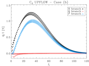
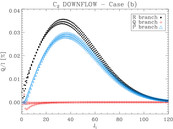
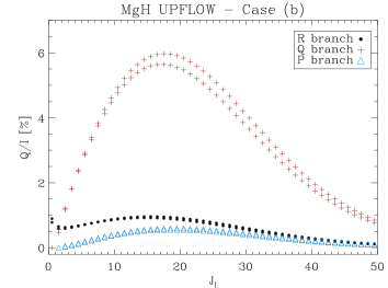
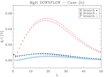
Figure 8.: This figure illustrates that the observed scattering polarization amplitudes in the P and R lines of the Swan system of C₂, and in the $Q$ lines of MgH, are coming mainly from the (granular) upflowing regions of the quiet solar photosphere. Although the height we chose for this illustration is 250 km, the height where $\tau_{\rm line-core}=1$ in a realistic model of the solar photosphere is smaller for the MgH lines than for the C₂ lines.

6.4. Applications of the Hanle-effect line-ratio technique for C₂ lines

Our analysis of the observations by Gandorfer (2000) of the scattering polarization signals of the C₂ lines with $J>20$ revealed very small depolarizations (see examples in the first three panels of Fig. 7). This led us to the conclusion that most of the volume of the photospheric regions that contribute to the observed molecular scattering polarization is occupied by very weak fields (Trujillo Bueno 2003a). In fact, during his talk at the SPW3, Trujillo Bueno already reported that the application of the Hanle-effect line-ratio technique to the C₂ lines suggests that $\langle B\rangle\approx 10$ G. A refined analysis leads us to conclude that $\langle B\rangle\approx 15$ G if we assume an exponential PDF, or $\langle B\rangle\approx 7$ G for the simpler case of a single value microturbulent field (Trujillo Bueno et al. 2004). So this technique proves itself a very powerful diagnostic tool for the investigation of “turbulent” magnetic fields, as it has been confirmed by other authors, who soon after SPW3 embraced the same technique to apply it to their investigations. For example, Berdyugina & Fluri (2004) applied it to three unblended C₂ lines that are thought to be more sensitive to the weaker fields (namely, the R${}_{1}(J=14)$ line with $B_{\rm H}\approx 4$ G, the R${}_{2}(J=13)$ line with $B_{\rm H}\approx 40$ G and the R${}_{3}(J=12)$ line with $B_{\rm H}\approx 4$ G). Note that using R${}_{2}(J=13)$ as a reference line is justified only if the mean field strength of the photospheric regions where the observed molecular scattering polarization is mainly produced is significantly smaller than 40 G. Fortunately, this is precisely the case (see Sect. 6.5, and Trujillo Bueno 2003a).

The R-triplet used by Berdyugina & Fluri (2004) is useful because the R₂ reference line is not blended with the R₁ line, which makes it easier to detect any possible magnetic depolarization (see the fourth panel of Fig. 7). They reported $\langle B\rangle\approx 15$ G for the case of a single value microturbulent field, as also did Faurobert & Arnaud (2003) via a complicated analysis of some of the C₂ lines with $J>20$ that we had previously considered. The disagreement with the value of 7 G determined by Trujillo Bueno et al. (2004) for the same model can be explained when we consider that both Berdyugina & Fluri (2004) and Faurobert & Arnaud (2003) overestimated the Einstein coefficients by a factor 2, overlooking the fact that $\Lambda$-doubling is not present in C₂ (see, e.g., Herzberg 1950, and Landi Degl’Innocenti 2006).

6.5. Which Regions Produce the Observed Molecular Scattering Polarization?

In the previous section, we showed how the analysis of the Hanle effect in the ${\rm C}_{2}$ lines of the Swan system also supports the hypothesis of a hidden magnetic field at sub-resolution scales. However it suggests a mean field strength $\langle B\rangle\sim 10$ G, which is much smaller than what is needed to explain the observations of the Sr i 4607 Å line presented earlier, which point instead to a hidden field with $\langle B\rangle\sim 100$ G. A resolution of this “enigma” was found when it was pointed out by Trujillo Bueno (2003a) that the observed scattering polarization in very weak spectral lines, such as those of C₂ and MgH, is coming mainly from the upflowing regions of the quiet solar photosphere (see also Fig. 2 of Trujillo Bueno et al. 2004). One way to illustrate this result is by using the single-scattering approximation formula

$$\frac{Q}{I}\approx\frac{3}{2\sqrt{2}}\,\frac{\eta_{I}^{l}}{\eta_{I}^{l}+\eta_{I}^{c}}\,\frac{S_{l}}{B_{\nu}}\,{\cal A}{\cal W}_{2}\;,$$ (3)

where most of the symbols have their usual meaning (e.g., ${\cal A}=J^{2}_{0}/J^{0}_{0}$ is the degree of anisotropy of the radiation field; cf. Trujillo Bueno 2003a), while ${\cal W}_{2}$ is the generalized polarizability factor defined by Landi Degl’Innocenti (2003) (see also Landi Degl’Innocenti 2006), which is the correct one for the astrophysical case (see Fig. 5 of Asensio Ramos & Trujillo Bueno 2003, for a comparison with the laboratory-case ${\cal W}_{2}$ used by Berdyugina et al. 2002). Figure 8 shows the $Q/I$ values we obtained by applying this formula with the physical conditions encountered at a height of 250 km in an upflowing cell center, and in a nearby downflowing intergranular lane, of a snapshot of the 3D hydrodynamical simulations of solar surface convection by Asplund et al. (2000).

In conclusion, the analysis of the scattering polarization observed without spatio-temporal resolution in C₂ and MgH lines is giving us empirical information on the distribution of hidden magnetic fields mainly in the (granular) upflowing regions of the quiet solar photosphere.

6.6. Evidence for a Fluctuating “Hidden” Field

First of all, it is important to point out that the calculated scattering polarization amplitude of the (moderately strong) Sr i 4607 Å line, for the zero-field reference case, gets significant contributions from both the upflowing and downflowing regions of the quiet solar photosphere. In contrast, we just showed that the scattering polarization of weak molecular lines, like C₂, is mainly produced in the (granular) upflowing regions, and we concluded from our analysis that these regions must be weakly magnetized, with $\langle B\rangle\sim 10$ G.

We now must ask how large the strength of the hidden field in the (intergranular) downflowing regions has to be, in order to be able to explain the inferred depolarization in the Sr i 4607 Å line. Interestingly, we find that the distribution of magnetic field strengths in the (intergranular) downflowing regions of the quiet solar photosphere must produce saturation for the Hanle effect in the Sr i 4607 Å line formed there. For this reason, Trujillo Bueno et al. (2004) concluded that the joint analysis of the Hanle effect in C₂ lines ($\langle B\rangle\sim 10$ G) and in the Sr i 4607 Å line ($\langle B\rangle\sim 100$ G) suggests that the strength of the hidden magnetic field “fluctuates” on the spatial scales of the solar granulation pattern, with much stronger fields above the intergranular regions.

The simplest intergranular PDF that produces Hanle-effect saturation for the Sr i 4607 Å line in the intergranular regions is that corresponding to a single value microturbulent field with $B\gtrsim 200$ G filling the entire downflowing volume. A more realistic scenario results when taking into account that the true intergranular PDF should have a tail towards the kG field strengths, as suggested by numerical experiments on turbulent dynamos and/or magnetoconvection. A merely illustrative example of an intergranular PDF that satisfies such requirements is the Maxwellian PDF used by Trujillo Bueno et al. (2004) for the downflowing regions of the quiet solar photosphere, ${\rm PDF}_{\rm downflows}=2.38\times 10^{-8}\,B^{2}\exp(-B/456)^{2}$, which we obtained by fitting with a Maxwellian the strong-field part of the intergranular histogram of the Zeeman splittings observed by Khomenko et al. (2003) in the Fe i lines at 1.56 $\mu$m. Note that this illustrative PDF implies that the filling factor of kG fields is $\sim 2\%$ of the downflowing volume—that is, it does not exclude the possibility of some kG field concentrations in the internetwork regions (Domínguez Cerdeña et al. 2003). We point out that with such a Maxwellian PDF for the downflowing plasma, most of the magnetic energy is carried by chaotic fields with strengths between the equipartition field values and $\sim 1$ kG. A similar conclusion is reached with other plausible choices for the intergranular PDF (e.g., a Gaussian), in so far that they satisfy the following constraints:

1. to produce saturation of the Hanle effect in the Sr i 4607 Å line;

2. to produce a Zeeman broadening of the intensity profiles of carefully-selected near-IR lines that is compatible with the observations.

Obviously, with the Hanle effect we cannot distinguish between two magnetic field strengths having $B>B_{\rm satur}$ (where $B_{\rm satur}\approx 200$ G for the Sr i 4607 Å line). For this reason, it is important to emphasize that a suitable way of constraining the parameters of the functional form chosen for the intergranular PDF is via a careful analysis of the Zeeman broadening of the intensity profiles of some carefully-selected near-IR lines that we have observed with the Tenerife Infrared Polarimeter.

6.7. Is Collisional Depolarization Significant for MgH and C₂?

We already showed how the analysis of the Hanle effect in the C₂ lines of the Swan system can be carried out by applying the Hanle-effect line-ratio technique for C₂ lines, which leads to the conclusion that $\langle B\rangle\sim 10$ G in the (granular) upflowing regions of the quiet solar photosphere (Trujillo Bueno 2003a; Trujillo Bueno et al. 2004). It is certainly fortunate that such technique is available, otherwise one would need a rather complex modeling of multilevel scattering polarization, given the fact that the two-level approximation is unsuitable for the C₂ lines (Landi Degl’Innocenti 2003; Asensio Ramos & Trujillo Bueno 2003).

Figure 9.: For the case dominated by collisional depolarization mentioned in the text, this figure shows the collisional depolarizing rate that is needed to fit the scattering polarization amplitude of each of the unblended MgH lines observed by Gandorfer (2000), for which $A_{ul}\approx 10^{7}\,\rm s^{-1}$. The fact that the ${\delta}_{u}$ values required for the best fit are almost insensitive to $J$, instead of being proportional to $J^{-1.5}$ as predicted by the theoretical work of Derouich (2006), suggests that the collisional depolarization inferred by Asensio Ramos & Trujillo Bueno (2005) is mainly caused by collisional transitions between different $J$-levels pertaining to the same vibrational and electronic state. While these types of collisional transitions are allowed for MgH, they are however strictly forbidden for C₂, which reinforces our conclusion that $\langle B\rangle\sim 10$ G in the upflowing regions of the quiet solar photosphere.

Which microturbulent mean field strength do we find via analysis of the observed scattering polarization signals in MgH lines? To answer this question we need a detailed 3D modeling, in order to be able to estimate correctly the amplitude of the zero-field linear polarization for each MgH line, which is produced by radiation scattering in the inhomogeneous solar photosphere. Fortunately, this 3D modeling of scattering polarization is feasible, since a two-level molecular model for each particular MgH line provides a reliable approximation. In fact, Asensio Ramos & Trujillo Bueno (2005) have recently solved the 3D scattering polarization problem in each of the 37 unblended MgH lines that show significant $Q/I$ amplitudes in the Second Solar Spectrum atlas of Gandorfer (2000). Their radiative transfer approach is similar to that pursued by Trujillo Bueno et al. (2004) for the Sr i 4607 Å line, adopting a realistic 3D model of the solar photosphere as it results from the hydrodynamic simulations of solar surface convection by Asplund et al. (2000). The aim was to investigate which combinations of field strengths and collisional depolarizing rates produce polarization amplitudes in agreement with the MgH observations of Gandorfer (2000). Asensio Ramos & Trujillo Bueno (2005) found that there are two possible regimes that lead to comparable best fits to the observed scattering polarization amplitudes:

1. a case dominated by collisional depolarization, but with the possibility of a weak microturbulent field whose strength cannot be much larger than 10 or 20 G (concerning the case of a single value field), in order to preserve the goodness of the best fit;

2. a strongly magnetized case characterized by a microturbulent field with strength greater than a few $10^{2}$ G, which nevertheless requires a small amount of collisional depolarization in order to attain the best fit.

Given that the observed scattering polarization comes mainly from the (granular) upflowing regions of the quiet solar photosphere, and that it is unrealistic to think that such regions are filled by a tangled magnetic field stronger than 100 G, Asensio Ramos & Trujillo Bueno (2005) opted for the first case dominated by collisional depolarization. Interestingly, this case is also characterized by relatively weak fields (see Note 10), so that it is compatible with the result of $\langle B\rangle\sim 10$ G that was obtained directly via the application of the Hanle-effect line-ratio technique for the C₂ lines of the Swan system. That result, however, was based on the assumption that collisional depolarization is unimportant for the upper levels of C₂ lines. If this were not the case, then the inferred mean field strength would be larger, given that in reality the magnetic field strength required to produce a sizable Hanle depolarization is approximately given by (e.g., Trujillo Bueno 2003a)

$$B\approx(1+{\delta_{u}})\,B_{\rm H}\,,$$ (4)

where $B_{\rm H}$ is given by Eq. (1), and ${\delta}_{u}=D^{(2)}\,t_{\rm life}\approx D^{(2)}/A_{ul}$. Therefore, it seems that, while collisional depolarization is essential for the MgH lines, in order to retrieve $\langle B\rangle\sim 10$ G, for the same reason it must be insignificant for the C₂ lines. We think that this is actually the case, given that C₂ is a homonuclear molecule in which collisional transitions between levels $J$ and $J\pm 1$ are strictly forbidden (see pages 131 and 238 of Herzberg 1950). In fact, as suggested by Fig. 9, this type of collisional transitions between nearby but different $J$-levels pertaining to the same vibrational and electronic state are probably the main cause of any collisional depolarization possibly occurring in the other molecular lines of the Second Solar Spectrum.

7. Conclusions and Outlook for the Future

A joint analysis of the Hanle effect in molecular lines and in the Sr i 4607 Å line leads to the conclusion that there is a vast amount of “hidden” magnetic energy and (unsigned) magnetic flux in the internetwork regions of the quiet solar photosphere, carried mainly by rather chaotic fields in the (intergranular) downflowing plasma with strengths $B>B_{\rm satur}\approx 200$ G. This result, complemented with the (upper-limit) constraint imposed by our analysis of the Zeeman broadening of the intensity profiles of carefully selected near-IR lines, suggests that most of this energy is actually carried by tangled magnetic fields at sub-resolution scales with strengths between the equipartition field values and $\sim 1$ kG. This hidden magnetic energy in the internetwork regions of the quiet Sun is larger than that corresponding to the kG fields of the supergranulation network, and is more than sufficient to compensate the radiative energy losses of the solar outer atmosphere (Trujillo Bueno et al. 2004).

Although the hidden magnetic field that we have discussed here carries most of the (unsigned) magnetic flux of the solar photosphere, we also must take into account the small-scale magnetic fields, with a filling factor of $\sim 1$%, that have been detected in the internetwork regions via the polarization induced by the Zeeman effect in Fe i lines (e.g. Domínguez Cerdeña et al. 2003; Khomenko et al. 2003; Sánchez Almeida et al. 2003b). Even though such magnetic fields make no significant contribution to the “observed” Hanle depolarization (because their filling factor is so small), they might still carry a significant fraction of the total magnetic energy, mainly if the observed circular polarization signals in the 6301.5 Å and 6302.5 Å lines of Fe i are really tracing kG fields concentrations, as claimed by Domínguez Cerdeña et al. (2006). Given that kG field concentrations in the internetwork regions of the quiet Sun would have a more obvious impact on the magnetic coupling with the outer atmosphere (e.g., Schrijver & Title 2003; Woo 2006), the determination of the true fraction of (internetwork) quiet Sun, occupied by magnetic fields with $B>1$ kG, should be a high-priority goal. In our opinion, a suitable strategy to achieve this goal is via a careful analysis of the Stokes profiles of some near-IR lines of Mn i that we have measured with the Tenerife Infrared Polarimeter.

The presence of all these small-scale magnetic fields in the quiet solar photosphere might have several important consequences for the overlying solar atmosphere, such as ubiquity of reconnecting current sheets and heating processes (e.g., Priest 2006). Therefore, it is now even more important to carry out detailed empirical investigations on the magnetism of the “quiet” solar chromosphere via a clever exploitation of a variety of subtle physical mechanisms by means of which a magnetic field can create and destroy spectral line polarization (e.g. Landi Degl’Innocenti & Landolfi 2004).

Acknowledgments.

We are grateful to R. Casini (HAO) for carefully reviewing our paper. This research has been funded by the Spanish Ministerio de Educación y Ciencia through project AYA2004-05792.

References

- Anderson & Athay (1989) Anderson, I. S., & Athay, R. G. 1989, ApJ, 346, 1010
- Asensio Ramos (2004) Asensio Ramos, A. 2004, Ph.D. Thesis, University of La Laguna, La Laguna, Tenerife, Spain
- Asensio Ramos & Trujillo Bueno (2003) Asensio Ramos, A., & Trujillo Bueno, J. 2003, in ASP Conf. Ser. Vol. 307, Solar Polarization 3, ed. J. Trujillo Bueno & J. Sánchez Almeida (San Francisco: ASP), 195
- Asensio Ramos & Trujillo Bueno (2005) Asensio Ramos, A., & Trujillo Bueno, J. 2005, ApJ, 635, L112
- Asplund et al. (2000) Asplund, M., Nordlund, Å., Trampedach, R., Allende-Prieto, C., & Stein, R. F. 2000, A&A, 359, 729
- Bellot Rubio & Collados (2003) Bellot Rubio, L., & Collados, M. 2003, A&A, 406, 357
- Berdyugina & Fluri (2004) Berdyugina, S. V., & Fluri, D. M. 2004, A&A, 417, 775
- Berdyugina et al. (2002) Berdyugina, S. V., Stenflo, J. O., & Gandorfer, A. 2002, A&A, 388, 1062
- Bommier & Molodij (2002) Bommier, V., & Molodij, G. 2002, A&A, 381, 241
- Bommier et al. (2005) Bommier, V., Derouich, M., Landi Degl’Innocenti, E., Molodij, G., & Sahal-Bréchot, S. 2005, A&A, 432, 295
- Cattaneo (1999) Cattaneo, F. 1999, ApJ, 515, L39
- de Wijn et al. (2005) De Wijn, A. G., Rutten, R. J., Haverkamp, E. M., & Sütterlin, P. 2005, A&A, 441, 1183
- Derouich (2006) Derouich, M. 2006, A&A, 449, 1
- Derouich, Sahal-Bréchot, & Barklem (2005) Derouich, M., Sahal-Bréchot, S., & Barklem, P. S. 2005, A&A, 434, 779