Cosmologies with dynamical and coupled Dark Energy vs. CMB data

Abstract

We compare a large set of cosmologies with WMAP data, performing a fit based on a MCMC algorithm. Besides of $\Lambda$CDM models, we take dynamical DE models, where DE and DM are uncoupled or coupled, both in the case of constant coupling and in the case when coupling varies with suitable laws. DE however arises from a scalar field self–interacting through a SUGRA potential. We find that the best fitting model is SUGRA dynamical DE, almost indipendently from the exponent $\alpha$ in the self–interaction potential.

The main target of this work are however coupled DE models, for which we find limits on the DE–DM coupling strength. In the case of variable coupling, we also find that greater values of the Hubble constant are preferred.

1 Introduction

Cosmologies with $\Omega_{o,de}\simeq 0.75$, $\Omega_{o,m}\simeq 0.25$, $\Omega_{o,b}\simeq 0.03$, $h\simeq 0.7$ and $n_{s}\simeq 1$ fit available data on CMB, LSS, and SNIa. Respectively, the above symbols are: the present density parameters for dark energy (DE), whole non–relativistic matter, baryons, the Hubble parameter in units of 100 km/s/Mpc, and the primeval spectral index. CMB is the Cosmic Microwave Background, LSS is the Large Scale Structure. Possible references for the above data are: Tegmark et al. (2001), De Bernardis et al. (2000), Hanany et al. (2000), Halverson et al. (2002), Spergel et al. (2003), Percival et al. (2002), Efstathiou et al. (2002), Riess et al. (1998), Perlmutter et al. (1999).

The nature of DE is not clear. This paper is devoted to comparing various hypotheses on its nature among them and with WMAP data. It is already known that, in order to fit data, DE must have a largely negative pressure: $p_{de}=w\rho_{de}$, with $-w\sim 0.7$–1 ($\rho_{de}$ is DE energy density). False vacua obey such a state equation with $w=-1$, but assuming DE to arise from false vacuum implies a fine–tuning of $\rho_{de}$, at the end of the EW phase transition by $1:10^{\,56}$. Otherwise, DE could be due to a self–interacting scalar field $\phi$ (Wetterich 1988, Ratra & Peebles 1988, RP hereafter). In this case we have dynamical DE (dDE) or quintessence.

The principal analysis of WMAP first–year data (Spergel et al., 2003) constrained flat $\Lambda$CDM models defined by six parameters: $\Omega_{o,b}h^{2}$, $\Omega_{o,m}h^{2}$, $h$, $n_{s}$, the fluctuation amplitude $A$ and the optical depth $\tau$. As possible extensions of $\Lambda$CDM cosmologies, several works considered models with a fixed state parameter $w\equiv p_{de}/\rho_{de}$ (Spergel et al. 2003, Bean et al. 2004, Tegmark et al. 2004, Melchiorri et al. 2004), or adopted $z$–dependent parameterizations of $w(z)$ interpolating between early–time and late–time values (Corasaniti et al. 2004, Jassal et al. 2005, Rapetti et al. 2004). A general conclusion was that current data mostly allow to constrain only the present state parameter, $w(z=0)\lesssim-0.80$. Here we shall extend the comparison to dDE models admitting a tracker solution.

Possible interactions of DE were also considered in the literature. Severe limits can be set to its interaction with baryons; Amendola (2000, 2003), Gasperini, Piazza & Veneziano (2002), Perrotta & Baccigalupi (2002), among others, discussed models where it interacts with Dark Matter (DM). Amendola & Quercellini (2003) performed a preliminary study on the limits on DE–DM interactions, arising from WMAP data, for DE theories with constant coupling (ccDE). It is also possible to consider cosmologies where the DM–DE coupling constant $C$, that we shall define below in accordance with Amendola (2000), is replaced by $1/\phi$ and is therefore variable in time (vcDE). A physical origin for these models was recently discussed by Mainini & Bonometto (2003; see also Colombo et al. 2003).

In this paper we perform a systematic fit of WMAP data to these different cosmologies: dDE, ccDE, vcDE, and $\Lambda$CDM. For the first 3 of them a SUGRA self–interaction potential will be taken (Brax & Martin 1999, 2000; Brax, Martin & Riazuelo 2000); its expression is given in Sec. 2 , together with essential information on coupled and uncoupled DE models. Further information on coupled models can be found, e.g., in Colombo et al. (2004).

The fit is performed by using a MCMC (MonteCarlo Markov Chain) algorithm, in the same way as the WMAP team fit the $\Lambda$CDM model. In Sec. 3, we describe the fitting procedure. In the case of that model we re–obtain their results.

The number of parameters to be fitted depends on the nature of the model. $\Lambda$CDM and vcDE models have the same number of parameters. In dDE models there is one extra parameter and ccDE models have a further parameter in respect to the previous cathegory. In evaluating the success of a fit, however, the number of parameters is taken into account. In Sec. 4 we perform sich comparison and in Sec. 5 we draw some conclusions.

2 The SUGRA potential

All models with dynamical DE we consider make use of a SUGRA potential

$$V(\phi)={\Lambda^{\alpha+4}\over\phi^{\alpha}}\exp\left(4\pi\phi^{2}\over m_{p}^{2}\right)$$ (1)

to yield the self–interaction of the scalar field $\phi$; here $m_{p}=G^{-1/2}$ is the Planck mass; $V$ depends on the two parameters $\Lambda$ and $\alpha$. When they are assigned, $\Omega_{de}$ is however fixed. We therefore prefere to use $\Omega_{de}$ and $\Lambda$ as independent parameters. The latter scale is related to $\alpha$ as shown in Figure 1, which holds also in the presence of DM–DE coupling.

Figure 1: Values of $\alpha$ corresponding to given $\Lambda$ scales in SUGRA models with $\Omega_{o,dm}=0.27$. The tiny differences, just above noise level, for coupled models ($\alpha_{\beta}$ and $\alpha_{1/\phi}$ for constant coupling and $\phi^{-1}$ coupling, respectively), are also shown.

The potential appears in the Lagrangian

$${\cal L}=\sqrt{-g}\left\{{1\over 2}g_{\mu\nu}\partial_{\mu}\phi\partial_{\nu}\phi-V(\phi)\right\}~{};$$ (2)

in the absence of coupling, the equation of motion

$$\ddot{\phi}+2{\dot{a}\over a}\dot{\phi}+a^{2}V^{\prime}(\phi)=0$$ (3)

follows, while the expressions for energy density $\rho_{\phi}=\rho_{\phi;kin}+\rho_{\phi;pot}$ and pressure $p_{\phi}=\rho_{\phi;kin}-\rho_{\phi;pot}$ are obtainable by combining the terms

$$\rho_{\phi,kin}={\dot{\phi}^{2}\over 2a^{2}}~{},~{}~{}\rho_{\phi,pot}=V(\phi)~{}.$$ (4)

In the radiation dominated era, eq. (3) admits the tracker solution

$$\phi^{\alpha+2}=g_{\alpha}\Lambda^{\alpha+4}a^{2}\tau^{2}~{},$$ (5)

with $g_{\alpha}=\alpha(\alpha+2)^{2}/4(\alpha+6)$. This tracker solution fairly defines the initial conditions also in the presence of coupling, although, in the presence of coupling, the equation of motion becomes

$$\ddot{\phi}+2{\dot{a}\over a}\dot{\phi}+a^{2}V^{\prime}(\phi)=Ca^{2}\rho_{c}$$ (6)

while CDM energy density varies according to the equation

$$\dot{\rho}_{c}+3{\dot{a}\over a}\rho_{v}=-Ca^{2}\rho_{c}~{};$$ (7)

baryon and radiation equations keep the usual shape. The coefficient $C$ sets the coupling strength and, in the case of constant coupling (ccDE), we can set

$$C=\left(\pi\over 3\right)^{1\over 2}{4\over m_{p}}\beta$$ (8)

so to parametrize the coupling strength through the adimensional coefficient $\beta$. Here we consider also a $\phi$–dependent coupling (vcDE)

$$C=\phi^{-1}$$ (9)

for which there is no extra parameter to fix the coupling strength.

3 Comparison with WMAP data through a MCMC algorithm

WMAP data have been extensively used to constrain cosmological parameters. They are high precision estimates of the anisotropy power spectrum $C_{l}^{T}$ up to $l\sim 900$, as well of the TE correlation power spectrum $C_{l}^{TE}$ up to $l\sim 450$. We shall fit these data to possible cosmologies, by considering a parameter space of 6 to 8 dimensions. A grid-based likelihood analysis would require a huge CPU time and we use a Markov Chain Monte Carlo (MCMC) approach, as it has become customary for CMB analysis (Christensen et al. 2001, Knox et al. 2001, Lewis et al. 2002, Kosowski et al. 2002, Dunkley et al. 2004).

To this aim, as in any attempt to fit CMB data to models, a linear code providing $C_{l}$’s is needed. Here we use our optimized extension of CMBFAST (Seljak & Zaldarriaga, 1996), able to inspect also ccDE and vcDE cosmologies. The likelihood of each model is then evaluated through the publicly available code by the WMAP team (Verde et al., 2003) and accompanying data (Hinshaw et al., 2003; Kogut et al., 2003).

A MCMC algorithm samples a known distribution ${\cal L}({\bf x})$ by means of an arbitrary trial distribution $p({\bf x})$. Here $\cal L$ is a likelihood and ${\bf x}$ is a point in the parameter space. The chain is started from a random position ${\bf x}$ and moves to a new position ${\bf x}^{\prime}$, according to the trial distribution. The probability of accepting the new point is given by ${\cal L}({\bf x}^{\prime})/{\cal L}({\bf x})$; if the new point is accepted, it is added to the chain and used as the starting position for a new step. If ${\bf x}^{\prime}$ is rejected, a replica of ${\bf x}$ is added to the chain and a new ${\bf x}^{\prime}$ is tested.

In the limit of infinitely long chains, the distribution of points sampled by a MCMC describes the underlying statistical process. Real chains, however, are finite and convergence criteria are critical. Moreover, a chain must be required to fully explore the high probability region in the parameter space. Statistical properties estimated using a chain which has yet to achieve good convergence or mixing may be misleading. Several methods exist to diagnose mixing and convergence, involving either single long chains or multiple chains starting from well separated points in the parameter space, as the one used here. Once a chain passes convergence tests, it is an accurate representation of the underlying distribution.

In order to ensure mixing, we run six chains of $\sim 30000$ points each, for each model category. We diagnose convergence by requiring that, for each parameter, the variances both of the single chains and of the whole set of chains ($W$ and $B$, respectively) satisfy the Gelman & Rubin test Verde et al. (2003); Gelman & Rubin (1992), $R<1.1$ with:

$$R={[(N-1)/N]W+(1+1/M)B\over W}~{}.$$ (10)

Here each chain has $2N$ points, but only the last $N$ points are used to estimate variances, and $M$ is the total number of chains. In most model categories considered, we find that the slowest parameter to converge is $\lambda$.

4 Results

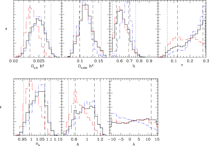
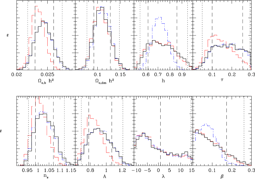
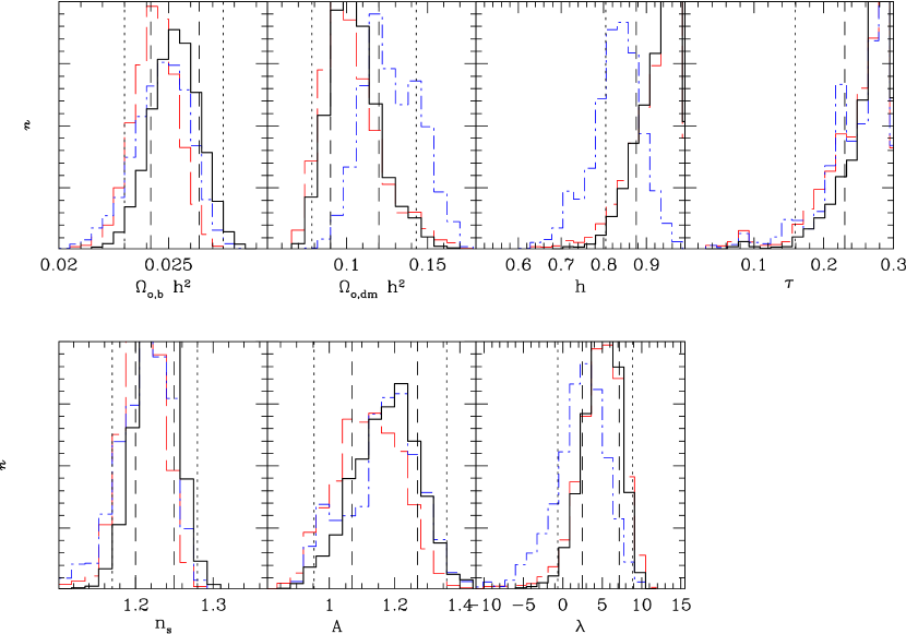
The basic results of this work are shown in the Tables 3–3. For each model category we provide the expectation values and the variance of each parameter, as well as the values of the parameters of the best fitting models. The corresponding marginalized distributions are plotted in figures 2–4, while joint 2D confidence regions are shown in figures 5–7.

The values of $\chi^{2}$ can also be compared, taking into account the number of degrees of freedom. This is shown in Table 4. The smallest $\chi^{2}$ is obtained for the uncoupled SUGRA model, which performs slightly better than $\Lambda$CDM.

Tables 1 and 2 and the corresponding figures, concerning uncoupled or constant–coupling SUGRA models, show that WMAP data scarcely constrain $\lambda=\log(\Lambda/{\rm GeV})$, allowed to vary from $\sim-12$ to 16. On the contrary, in the case of a $\phi^{-1}$ coupling, loose but precise limitations on $\lambda$ are set, as is shown in Table 3. In the presence of this coupling, the 2–$\sigma$ $\Lambda$–interval ranges from $\sim 10$ to $\sim 3\cdot 10^{10}$GeV.

Table 1: SUGRA parameters for dDE models: for each parameter $x$, the expectation value $\langle x\rangle$, its variance $\sigma_{x}$, and its maximum likelihood value $x_{max}$, in the 7–dimensional parameter space, are shown.

$x$	$\langle x\rangle$	$\sigma_{x}$	$x_{max}$
$\Omega_{o,b}h^{2}$	0.025	0.001	0.026
$\Omega_{o,dm}h^{2}$	0.12	0.02	0.11
$h$	0.63	0.06	0.58
$\tau$	0.21	0.07	0.28
$n_{s}$	1.04	0.04	1.08
$A$	0.97	0.13	1.11
$\lambda$	3.0	7.7	13.7

Table 2: SUGRA parameters for ccDE models; the parameter space is 7–dimensional and parameter are shown as in the previous Table.

$x$	$\langle x\rangle$	$\sigma_{x}$	$x_{max}$
$\Omega_{o,b}h^{2}$	0.024	0.001	0.024
$\Omega_{o,dm}h^{2}$	0.11	0.02	0.12
$h$	0.74	0.11	0.57
$\tau$	0.18	0.07	0.17
$n_{s}$	1.03	0.04	1.02
$A$	0.92	0.14	0.93
$\lambda$	-0.5	7.6	8.3
$\beta$	0.10	0.07	0.07

Table 3: SUGRA parameters for vcDE models. At variance from other model categories, $\lambda$ here is constrained. Parameter values are shown as in Table 1.

$x$	$\langle x\rangle$	$\sigma_{x}$	$x_{max}$
$\Omega_{o,b}h^{2}$	0.025	0.001	0.026
$\Omega_{o,dm}h^{2}$	0.11	0.02	0.09
$h$	0.93	0.05	0.98
$\tau$	0.26	0.04	0.29
$n_{s}$	1.23	0.04	1.23
$A$	1.17	0.10	1.20
$\lambda$	4.8	2.4	5.7

Figure 2: Marginalized distributions for the 7–parameters SUGRA model with no priors (solid lines), BBNS prior (long dashed) or HST prior (dot–dashed). Short dashed (dotted) vertical lines show the boundaries of 68.3 % c.l. (95.4 % c.l.) interval; for $\lambda$ only upper limits are shown.

Table 4: Goodness of fit. We lists the number of degrees of freedom (d.o.f.), the reduced $\chi^{2}_{eff}$, and the corresponding probability of the best–fit model. $\Lambda$CDM models have 1342 degrees of freedom, uncoupled and vcDE models have 1341, while ccDE models have 1340.

	$\chi^{2}_{eff}$	prob.
dDE	1.062	5.2 %
ccDE	1.066	4.7 %
vcDE	1.074	2.9 %
$\Lambda$CDM	1.066	4.7 %

Figure 3: As Fig. 2 but for the 8–parameters ccDE model. For $\lambda$ and $\beta$ only the upper c.l. boundaries are shown.

Figure 4: As Fig. 2 but for the 7–parameters vcDE model.

Figure 5: Joint 2D constraints for SUGRA models. Light (dark) shaded areas delimit the region enclosing 68.3 % (95.4 %) of the total points.

Figure 6: As Fig. 5 but for ccDE models.

Figure 7: As Fig. 5 but for vcDE models. Here, cosmological parameters are more stringently constrained than in other models.

Figure 8: $C_{l}^{T}$ spectra for the best fit SUGRA (solid line), ccDE (dotted line) and vcDE (dashed). Dual–axion (dot–dashed) models are also shown; they can be considered a particular case within vcDE models, for which $10\leq\lambda\leq 10.5$ (see text). The binned first–year WMAP data are also plotted.

Figure 9: Best fit $C_{l}^{TE}$ spectra.

Figure 10: Best fit $C_{l}^{E}$ spectra.

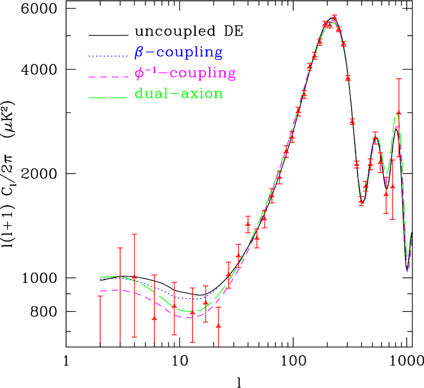
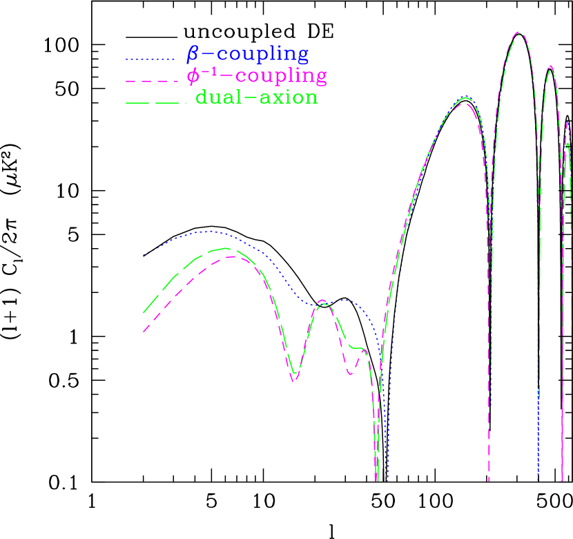
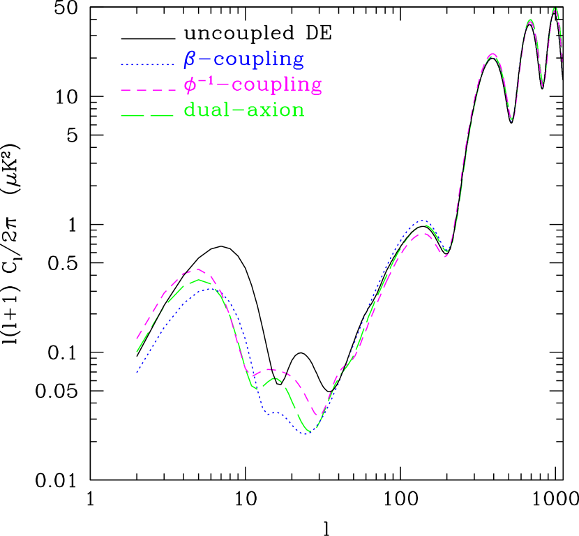
These constraints apparently arise from polarization data: when DE begins to affect cosmic expansion, the $\phi$ evolution acts on DE density and pressure, as well as on its coupling, and requires an $l$–dependence of multipole amplitudes ablt to meet data only for a limited range of $\Lambda$ values. This can be noticed in Figures 8 and 9, where the best–fit $C_{l}^{T}$ and $C_{l}^{TE}$ spectra for all best–fit models (apart of $\Lambda$CDM) are compared.

Fig. 8 also shows why no model neatly prevails. At large $l$ all best–fit models yield similar behaviors. Discrimination could be improved only through better large angular scale observations, especially for polarization, able to reduce errors on small–$l$ harmonics.

5 Discussion

5.1 Uncoupled SUGRA models

SUGRA uncoupled models are found to be consistent with WMAP data. The ratio $w=p/\rho$, for these models is typically $\lesssim-0.80$ at $z=0$. However, they exhibit a fast variation of $w$, which is already $\sim-0.6$ at $z\sim 1$–2. Such a decrease, however, does not cause a conflict with data and these models perform even better than $\Lambda$CDM.

We also considered the effect of adding some priors. For uncoupled or constant–coupling SUGRA models, the analysis in the presence of priors leads to analogous conclusions. There are however variations in the estimate of cosmological parameters. First, the opacity $\tau$ is pushed to values exceeding the $\Lambda$CDM estimates (see also Corasaniti at al. 2004). This can be understood in two complementary ways: (i) ISW effect is stronger for dDE than for $\Lambda$CDM, as the field $\phi$ evolves during the expansion; hence, DE effects extend to a greater redshift, increasing $C_{l}^{T}$ values in the low–$l$ plateau (e.g., Weller & Lewis, 2003). To compensate this effect the fit tends to shift $n_{s}$ greater values. Owing to the $\tau$–$n$ degeneracy, this is then balanced by increasing $\tau$. (ii) It must also be reminded that the expected TE correlation for dDE, at low $l$, is smaller (Colombo et al. 2003). Then, when TE correlation data is included, a given correlation level is fit by a greater $\tau$. In any case, however, $\tau\sim 0.07$ keeps consistent with data within less than 2–$\sigma$’s.

Greater $\tau$’s affect also $\Omega_{b}h^{2}$ estimates, whose best–fit value is then greater, although consistent with $\Lambda$CDM within 1–$\sigma$. Adding a prior on $\Omega_{b}h^{2}=0.0214\pm 0.0020$ (BBNS estimates (Kirkman et al., 2003)) lowers $h$, slightly below HST findings, but still well within 1–$\sigma$. We therefore consider the effect of adding a prior also on $h$.

The effects of these priors are shown in Figures 2 and 3. The new distributions are given by the dashed red line (prior on $\Omega_{b}h^{2}$) and the dot–dashed blue line (prior on $h$). The former prior affects mainly $\tau$ and $n_{s}$; $\tau$ and $n_{s}$ are lowered to match WMAP’s findings, the high tail of $\tau$ distribution is partly suppressed. The physical analysis of primeval objects causing reionization (Ciardi et al. 2003, Ricotti et al. 2004). which are still allowed but certainly not required.

5.2 ccDE SUGRA models

The latter prior favors greater $h$ values. In the absence of coupling, this favors low–$\lambda$ models, closer to $\Lambda$CDM. In fact, the sound horizon at decoupling is not affected by the energy scale $\Lambda$, while the comoving distance to last scattering band is smaller for greater $\lambda$’s. Then, for greater $\lambda$’s lower $h$ values are favored, so to meet the first peak. In the presence of coupling, there is a simultaneous effect on $\beta$: greater $\beta$’s yield a smaller sound horizon at recombination, so that the distribution on $h$ is smoother.

A previous analysis of WMAP limits on constant coupling models had been carried on by Amendola & Quercellini (2003). Their analysis concerned potentials $V$ fulfilling the relation $dV/d\phi=BV^{N}$, with suitable $B$ and $N$. Furthermore, they assume that $\tau\equiv 0.17$. Our analysis deals with a different potential and allows more general parameter variations. The constraints on $\beta$ we find are less severe. It must be however outlined that $\beta\mathrel{\mathchoice{\lower 0.5pt\vbox{\halign{$\mathnew\displaystyle\hfil#\hfil$\cr>\crcr\sim\crcr}}}{\lower 0.5pt\vbox{\halign{$\mathnew\textstyle\hfil#\hfil$\cr>\crcr\sim\crcr}}}{\lower 0.5pt\vbox{\halign{$\mathnew\scriptstyle\hfil#\hfil$\cr>\crcr\sim\crcr}}}{\lower 0.5pt\vbox{\halign{$\mathnew\scriptscriptstyle\hfil#\hfil$\cr>\crcr\sim\crcr}}}}0.1$–0.2 seem however forbidden by a non–linear analysis of structure formation (Macciò et al. 2004).

5.3 vcDE SUGRA models

The main peculiarity of $\phi^{-1}$–models is that, although the $\xi^{2}$ value is not much worsened in respect to other cases, parameters are more strongly constrained in this caseq. This is evident in Fig. 7. In particular, at variance from the former case, the energy scale $\Lambda$ is significantly constrained.

Several other parameters are constrained, similarly to coupled or uncoupled SUGRA models. What is peculiar of $\phi^{-1}$–models is the range of $h$ values which turn out to be favored. The best–fit 2–$\sigma$ interval does not extend much below 0.85 .

This is a problem for these models in their present form. Should new data support a greater $h$ value, vcDE models would however be favored. Quite in general, however, we must remind that vcDE models were considered here only in association with a SUGRA potential; vcDE models with different potentials can possibly agree with a smaller $h$.

5.4 Dual axion models

A particular but significant case, among vcDE models, are dual axion models (DAM; for a detailed analysis see Mainini & Bonometto 2004, Colombo et al 2004).

These models arise from a generalization of the PQ solution of the strong–$CP$ problem (Peccei & Quinn 1977), obtained by replacing the NG potential acting on a complex scalar field $\Phi$ with a quintessence potential admitting a tracker solution. While, in the usual PQ approach and its generalization, only the phase $\theta$ of the $\Phi$ field is physically sgnificant, in the DAM also its modulus $\phi$ is physically observable. In both cases, quanta of the $\theta$ field are axions and, if DM is made of axions, its density parameter $\Omega_{o,m}$ is set either by the $F_{PQ}$ parameter, in the NG potential, or by the energy scale $\Lambda$, in the quintessence potential. In the latter case, therefore, both DM and DE features follow from fixing the single parameter $\Lambda$.

A detailed analysis of DAM shows that it belongs to the set of vcDE cosmologies; its main peculiarity is that $\lambda$ and $\Omega_{o,m}$ are no longer independent degrees of freedom. Henceforth, this model is strongly constrained and depends on the same number of parameters as SCDM. By varying $\Omega_{o,m}$ in its physical range, $\lambda$ keeps however close to 10. This great value of $\lambda$ therefore causes a conflict with the observed $h$ range. All previous comments on vcDE models however hold, while it is also possible that extra contribution to DM, arising from topological singularities expected in axion theories, can ease the $h$ problem.

6 Conclusions

The first evidences of DM are fairly old; they date some 70 years ago. However, only in the late Seventies limits on CMB anisotropies showed that non–baryonic DM had to be dominant. DE can also be dated back to Einstein’s cosmological constant, although only SN Ia data revived it, soon followed by data on CMB and deep galaxy samples.

The main topic of this paper is the fit of WMAP data with various DE models: $\Lambda$CDM, SUGRA dynamical and constant coupling DE models, as well as variable coupling DE models. In the last model DM and DE are coupled in a non–parametric way, with $C=\phi^{-1}$.

The fits of WMAP data to these models yield similar $\chi^{2}$’s. At variance from other model categories, however, in vcDE models, CMB data constrain $\Lambda$. This is due to the stronger effects of $\phi$ variations on the detailed ISW effect, as they affect both DE pressure and energy density, as well as DE–DM coupling. In principle, this strong impact of $\phi$ variation could badly disrupt the fit and make vcDE models significantly farther from data. It is noticeable that this does not occur.

The success of vcDE models would be complete if the favored range of values of the Hubble parameter ($h\sim 0.8$–1) could be slightly lowered. This range is however obtained just for a SUGRA potential. Furthermore, primeval fluctuations were assumed to be strictly adiabatic while, in axion models, a contribution from isocurvature modes can be expected. This could legitimately affect the apparent position of the first peak in the anisotropy spectrum, so completing the success of the model, in a fully self–consistent way.

References

- Amendola (2000) Amendola L. 2000, Phys.Rev D 62, 043511
- Amendola (2003) Amendola L. 2003 Phys.Rev.D 69, 103524
- Amendola & Quercellini (2003) Amendola L. & Quercellini C. 2003, Phys. Rev. D69, 023514
- Bean & Dorè (2004) Bean R. & Dorè O 2004, Phys.Rev. D69, 083503
- Brax & Martin (1999) Brax P. & Martin J., 1999, Phys.Lett. B468, 40
- Brax & Martin (2000) Brax P. & Martin J., 2000, Phys.Rev.D 61, 103502
- Brax, Martin & Riazuelo (2000) Brax P., Martin J. & Riazuelo A., 2000, Phys.Rev.D 62, 103505
- Christensen et al. (2001) Christensen N., Meyer R., Knox L. & Luey, B. 2001, Classical and Quantum Gravity, 18, 2677
- Ciardi et al. (2003) Ciardi B., Ferrara A. & White S.D.M. 2003, MNRAS, 344, L7
- Colombo (2004) Colombo L.P.L. 2004, JCAP, 3, 003
- Colombo et al. (2003) Colombo L.P.L., Mainini R. & Bonometto S.A. 2003, in proceedings of Marseille 2003 Meeting, ’When Cosmology and Fundamental Physics meet’
- Corasaniti et al. (2004) Corasaniti P.S., et al. 2004, Phys.Rev.D 70, 083006
- De Bernardis et al. (2000) De Bernardis et al., 2000 Nature 404, 955
- Dunkley et al. (2004) Dunkley J., et al. 2004, MNRAS 356, 285.
- Efstathiou et al. (2002) Efstathiou, G. et al., 2002, MNRAS, 330, 29
- Gelman & Rubin (1992) Gelman A. & Rubin D.B., 1992, Statist. Sci. 7, 457
- Gasperini et al. (2002) Gasperini M., Piazza F. & Veneziano G., 2002, Phys. Rev. D65, 023508
- Halverson et al. (2002) Halverson N.W. et al. 2002, ApJ 568, 38
- Hanany et al. (2000) Hanany S. et al, 2000, ApJ 545, L5
- Hinshaw et al. (2003) Hinshaw G., et al. 2003, ApJ Suppl., 148, 135
- Jassal et al. (2005) Jassal H.K., Bagla J.S., & Padmanabhan T. 2005 MNRAS 356, L11
- Kirkman et al. (2003) Kirkman D. et al. 2003, ApJS, 149, 1
- Knox et al. (2001) Knox L., Christensen, N. & Skordis C. 2001, ApJ 63, L95
- Kogut et al. (2003) Kogut A., et al. 2003, ApJ Suppl., 148, 161
- Kosowski et al. (2002) Kosowsky A., Milosavljevic M. & Jimenez R. 2002, Phys.Rev.D 66, 63007
- Lewis et al. (2002) Lewis, A. & Bridle, S. 2002, Phys.Rev. D 66, 103511
- Macciò et al. (2004) Macciò A., Quercellini C., Mainini R., Amendola L. & Bonometto S.A. 2004, Phys. Rev. D69, 123516
- Mainini & Bonometto (2004) Mainini, R. & Bonometto S.A., 2004, Phys. Rev. Lett. 93, 121301
- Melchiorri (2004) Melchiorri A. 2004 Plenary Talk given at Exploring the Universe (Moriond 2004), La Thuile, March 28 - April 4, 2004 Preprint astro–ph/0406652
- Peccei & Quinn (1977) Peccei R.D. & Quinn H.R. 1977, Phys.Rev.Lett. 38, 1440;
- Percival et al. (2002) Percival W.J. et al., 2002, MNRAS 337, 1068
- Perlmutter et al. (1999) Perlmutter S. et al., 1999, ApJ, 517, 565
- Perrotta & Baccigalupi (2002) Perrotta F. & Baacigalupi C., 2002, Phys. Rev. D65, 123505
- Rapetti et al. (2004) Rapetti D., Allen S.W., & Weller J. 2005, MNRAS 360, 555
- Ratra & Peebles (1988) Ratra B. & Peebles P.J.E., 1988, Phys.Rev.D 37, 3406
- Ricotti & Ostriker (2004) Ricotti M. & Ostriker J.P. 2004, MNRAS, 350, 359
- Riess et al. (1998) Riess, A.G. et al., 1998, AJ116, 1009
- Seljak & Zaldarriaga (1996) Seljak U. & Zaldarriaga M. 1996, ApJ, 469 437
- Spergel et al. (2003) Spergel D.N. et al., 2003, ApJ Suppl. 148, 175
- Tegmark et al. (2004) Tegmark M., et al. 2004, Phys.Rev. D69, 10350
- Tegmark et al. (2001) Tegmark M., Zaldarriaga M. & Hamilton, 2001 Phys.Rev.D 63, 43007
- Verde et al. (2003) Verde et al. 2003, ApJ Suppl., 148, 195
- Weller & Lewis (2003) Weller J. & Lewis A.M. 2003, MNRAS, 346, 987
- Wetterich (1988) Wetterich C. 1988, Nucl.Phys.B 302, 668