Bernd Inhester
Max-Planck-Institute for Solar System Research
37191 Katlenburg-Lindau, Germany draft version,  8^nd August 2006,   to appear as an ISSI publication

We discuss some basic principles of stereoscopy and their relevance to the reconstruction of coronal loops. The aim of the paper is to make the solar physicist familiar with basic stereoscopy principles and to give hints how they may apply to the analysis of data from the forthcoming STEREO mission. We disucss the geometry of the solar coronal stereo problem, give the basic principles of a tie-point reconstruction algorithm and consider ambiguities and resolution errors. Finally we mention extensions to plain stereoscopy such as a third view, a tomography-like approach and how magnetic field information can be used to improve the reconstruction.

1 Introduction

One of the first applications of stereoscopy in space and astrophysics was the determination of the distance of near-by stars by measuring the parallax angle. Even though stereoscopy is now applied to much more complex objects, the essential reconstruction principles still remain the same. Once an object is detected and identified in two images from different vantage points, the reconstruction is a purely linear geometrical task.

However, the most challenging problem associated with stereoscopy precedes the geometrical reconstruction step: the identification and matching of the objects to be reconstructed in the stereo images. But even before we start to talk about identification, matching and reconstruction, we have to be concerned about which are the objects that we hope to find in the images.

This text is strongly devoted to solar physics and especially meant as background for STEREO mission scientists. On the other hand, our intention here is to draw parallels to and learn from other fields of physics and engineering where stereoscopy has been applied for a long time.

The classical stereoscopy problem is the reconstruction of surfaces from a pair of images. For complicated surfaces such as, e.g., human faces this is a formidable task and not possible without well calibrated images and highly specialized information beyond the image data alone, e.g., the location of light sources and the reflectivity of the human skin.

A more elementary task is the reconstruction of simple geometrical objects composed of piecewise planes connected by straight edges. The reconstruction in this case can already be achieved if the only edges can be identified in the images. They usually show up as sharp boundaries in brightness, colour or texture – the absolute values of the brightness, colour or texture are not needed. Subsequently, the edges are reconstructed first and hopefully, suitably connected edges lie in planes which then bound the desired surfaces.

Figure 1: Backprojection to reconstruct point-like, curve-like and surface-like objects to demonstrate the different conditions of solvability.

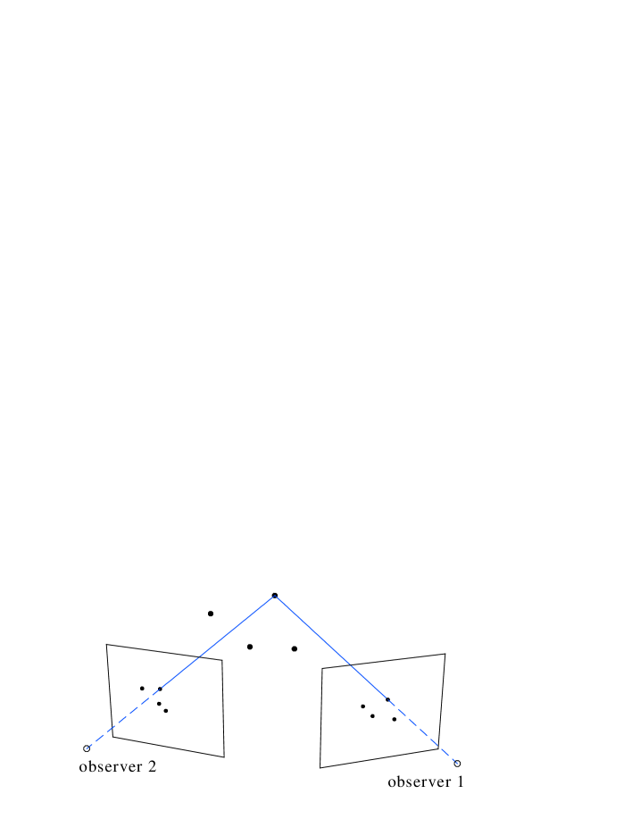
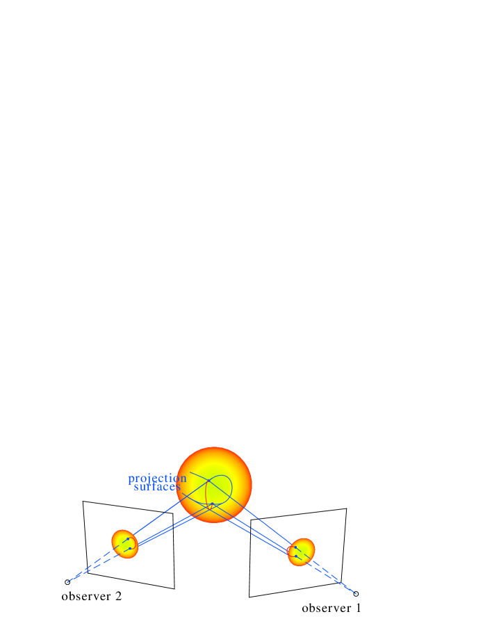
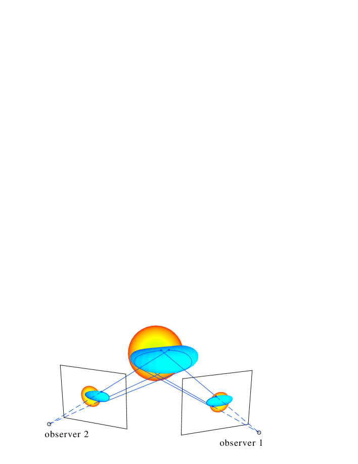
There is a good reason why the edges are the natural objects to be reconstructed first. If have identified an object, the reconstruction task, i.e., the calculation of its depth, depends on the extent or dimension of the object:

• For a point-like object, we extract 2$\times$2 image coordinates from the image pair from which we determine by a linear relationship the 3 space coordinates of the object – a clearly overdetermined mathematical problem (Fig. 1a).

• For a curve-like object, we extract two two-dimensional curves from the image pair, each of which could be considered the “head-on” image of a projection surface extending in the respective view direction. The intersection of the two projection surfaces yields (in the ideal case) a unique three-dimensional curve, the desired result of our reconstruction (Fig. 1b).

• For a surface-like objects, we can its extract visible edges from the image pair, but as we see in Fig. 1, the respective projection surfaces refer to different locations on the surface to be reconstructed. Our problem is obviously underdetermined and without further information, e.g., the assumption of a surface curvature or the knowledge about the location of a light source, the surface reflectivity together with precise intensity measurements, a reconstruction is impossible (Fig. 1c).

Hence there is a good reason why in classical stereoscopy the edges, which are curve-like objects, are reconstructed first. On the solar surface similar objects which lend themselves to being reconstructed are striated plasma structures extending along the coronal magnetic field. Already the first applications of stereoscopy in solar physics by Berton and Sakurai (1985) and Kouchmy and Molodensky (1992) considered active region loops and plasma striations in white-light coronagraph observations.

The solar corona is dominated both dynamically and statically by its magnetic field. The visible striations above the solar surface are essentially shaped by the efficient transport properties along the field lines and are therefore smoothly curved. When talking about three-dimensional curves as objects of reconstruction, we will have these plasma structures in mind. Below we will explicitly discuss loops, which are plasma striations on presumably closed magnetic field lines, and plumes, i.e., elongated density enhancements on open field lines, visible over the polar coronal holes preferentially at times of the solar activity minimum.

The loops clearly show up in EUV images of the solar corona since the about 1 million K hot coronal plasma confined on thin flux tubes emits much stronger in EUV wavelengths then the cool solar surface of only 5600 K. The high contrast is probably due to both drastic temperature and density variations across coronal field lines. Note that the resulting variation in pressure is still small compared to the shape-forming forces of the magnetic field. The huge temperature difference between the corona and the lower atmosphere layers largely eliminates backround radiation from these lower layers so that the large intrinsic contrast of coronal loops is preserved even though the plasma density in the corona is by orders of magnitude smaller than the density at the surface.

Plumes have less contrast but are seen in optical and EUV wavelengths, probably, because their enhanced emission is due to an enhanced density on some polar field lines an not so much due to a drastic temperature change. Best contrast is obtained where the plumes extend beyond the visible solar disk and can be observed against the dark background sky.

We will start with introducing the natural geometry attached to stereoscopic observations. The epipolar coordinate system thereby introduced is already a first step towards the important task to associate features from both images with each other. This task, as mentioned above, is formidable and is outlined in the third section. Much of the research in various fields of stereoscopy is devoted to this step and especially for solar observations there is still much work ahead on this special problem. The geometrical reconstruction task itself is elaborated in some depth in the tie-point method chapter. Even the geometrical reconstruction can fool the unaware user and the topics of the following sections deal with the precision of the reconstruction and the uniqueness of whatever we hope to obtain as final result. Additional observations, e.g., a “third eye”, magnetic field observations, and alternative methods and constraints to the geometrical reconstruction such as the tomography approach are discussed at the end.

All these latter methods together with our basic knowledge of physics should be seriously considered as additional potential constraints when analysing images whenever possible. We should keep in mind that the step from images, i.e., 2D projections to the 3D real world is often underestimated. As humans we percieve our 3D environment largely through the images produced on the focal plane of our eyes. We have calibrated our sense of depth in early childhood and we have for years classified the objects which surround us in every day life. Whenever we see a projection of one of these objects we immediately associate this limited projection with the 3D-idea of this object we have stored in our brain. Most often we are not aware any more of this process and we therefore tend to consider 2D projections and their 3D shape as equivalent. But if we want to teach a computer to make a 3D reconstruction, we have to give this additional information to him explicitly. Even worse, in space we still largely lack this important background of information and we so find ourselves in this area still “in the childhood of perception”.

2 Epipolar geometry and Rectification

The first step is to find a suitable coordinate system so that the reconstruction can be reduced from a three-dimensional to a set of two-dimensional planar problems. A similar strategy is known from tomography where the reconstruction can be obtained first for a dense set of planes normal to the rotation axis of the object (or the camera). The final three-dimensional model is then interpolated in between these planes. A necessary condition for the validity of this procedure is that the rotation axis lies normal to the plane of view directions and that affine geometry for the camera projection rays can be assumed.

Figure 2: Orientation of epipolar planes in space and the respective epipolar lines in the images for two observers (e.g., space craft) looking at the Sun. The observers telescope screens are derived from a projective geometry camera model.

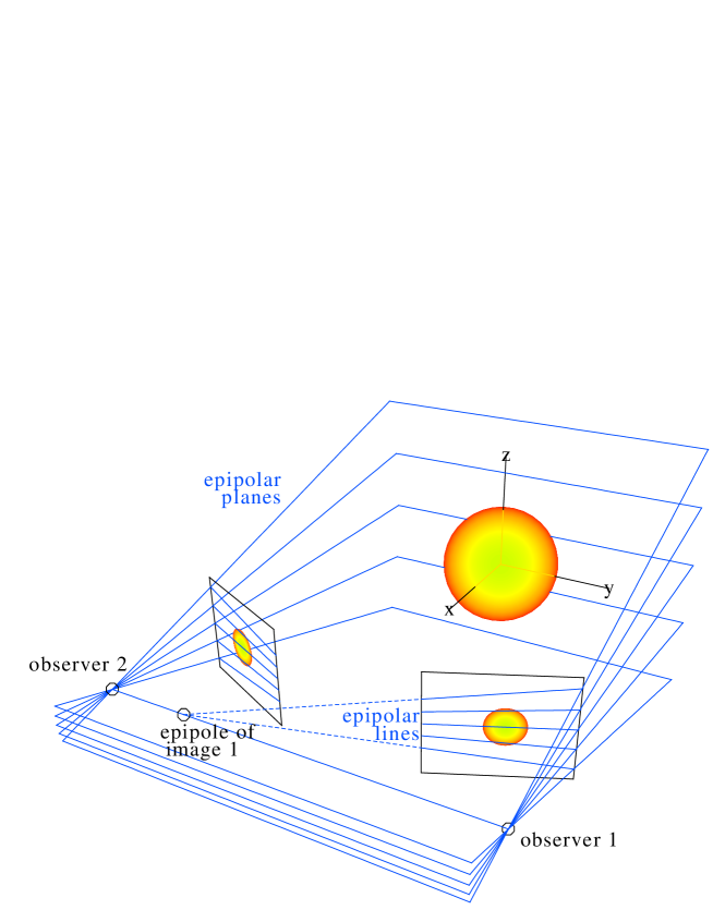
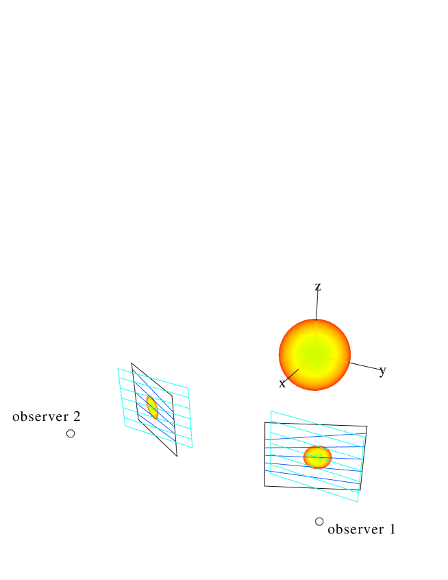
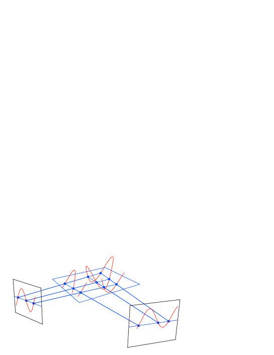
For stereoscopy the geometrical conditions for this segmentation of space are much more relaxed because only two view points and two view directions are involved. The line connecting the view points is called the stereo base line, which subtends the stereo base angle between the two main view directions (more precisely, the optical axes of the respective telescope. Note that the two optical axes do not need to intersect). The two observer positions and any object point to be reconstructed exactly define a plane. For many object points there are many planes but all have in common that they contain the two observer positions. Any of this set of planes which contains the two observer positions is called an epipolar plane and these planes form a natural geometrical basis for our reconstruction coordinate system (see Fig. 2).

By the above definition, epipolar planes project on both observer’s images as lines: since any observer himself is on any epipolar plane, he sees them “head on”. These lines are called accordingly the epipolar lines and they generate a natural coordinate system on the image planes.

Depending on his field of view, one observer, say observer 1, may see observer 2. Since observer 2 is defined to lie on all epipolar planes, all epipolar lines in image 1 must converge in the projection of observer 2, called the epipole of the respective projection.

The epipolar lines in each image can easily be determined from the observers positions and the direction of their optical axes. Note that the epipolar lines in one image always depend on the position of both observers, hence any change in position of observer 2 requires a redetermination of epipolar lines also in image 1. The epipolar lines may be labelled by the angle they make with respect to a reference epipolar plane or by the coordinate of the plane’s intersection with a suitable axis of a completely independent coordinate system, e.g., the $z$-axis in Fig. 2. In the STEREO context, a suitable axis is the rotation axis of the Sun. Since the space craft are more or less close to the ecliptic, the Sun’s rotation axis should intersect all relevant epipolar planes. This way, an epipolar plane is uniquely defined by the two observer’s positions and the intersection point.

Conversely, most space points lie on a unique epipolar plane. The only exception are points on the stereo base line which connects the two observers. In fact there is no depth reconstruction possible for points on this line. If we rule them out, any point identified in one image on a certain epipolar line must occur on the same epipolar line in the other image.

This straight forward geometrical consequence is known as epipolar constraint. It enormously helps the reconstruction since, in principle, we can directly overplot the epipolar lines and their labels onto each image and thus read the epipolar plane of an object from the image. Hence, we are only left with calculating the object’s two-dimensional coordinates on the known epipolar plane. This can be achieved from measuring the positions of the object’s projection along the epipolar line in either image. The depth of an object in particular is proportional to the difference of these coordinate values along the epipolar line of the two projections, the so-called disparity (for a quantitative definition see section 4).

From the geometrical construction it is clear that epipolar lines usually are not parallel. In the case of the STEREO spacecrafts at about 1 AU the visible epipolar lines typically make angles of $\mathcal{O}(\mathrm{atan}~{}1R_{\odot})/1\mathrm{AU}$ $\simeq$ 0.01 in an EUVI image concentrated on the solar disk. For the HI images, on the other hand, the epipoles come into the field of view and epipolar lines in the image may make angles of $\mathcal{O}(1)$.

Figure 3: Virtual change of orientation of the observer’s main view direction equivalent to rectification. The rectified configuration is indicated by the rotated screens drawn in light blue.

For ease of reconstruction it would be desirable to have the epipolar lines mapped into horizontal lines. This corresponds to the case when both spacecrafts would have their optical axes directed parallel to each other (see Fig.3). The transformation of a general image pair to an pair with horizontal epipolar lines is called rectification. Usually, this step includes also the elimination of distortion effects from the image. Note that in presence of a distorted image mapping, epipolar lines may not be straight in the original image. In rectified images, a space point maps to the same vertical image coordinate in both images. Hence the image reconstruction can be performed row by row.

Whether the stereo image pair is rectified or not – the epipolar constraint is a strong geometrical constraint and has to be obeyed whatever reconstruction algorithm is employed. Using the epipolar coordinates explicitely reduces the three-dimensional reconstruction problem to a set of two-dimensional problems.

3 Identification and Matching

The matching problem consists of correctly identifying the projections of an object in the two stereo images. The relationship thus established between the projections is called a correspondence. We will discuss further below in section 6 what the consequences are if the problem is not solved properly before the reconstruction is made. In general, ghost signals will appear and one possible approach is to perform the matching imperfectly as good as possible and select remaining ghosts afterwards in the reconstructed three-dimensional model. This post-processing selection must then be based on a-priori known properties of the reconstructed objects – we hence incorporate additional information beyond the image data into our problem. To some extent, this approach will be discussed below in sections 6 and 8.

On the other hand, it would of course be desirable to add this knowledge already at the matching stage before the reconstruction is made. Therefore solutions to the matching problem are often strongly tailored to the specific objects observed. EUV and coronagraph images of the solar corona often show a mess of loops and structures and their identification is a hard task indeed. For the STEREO mission, these rules and tools still have to be developed to a large extent and we can give here only some general recommendations.

The methods to find correspondences between the stereo images used in classical stereoscopy are generally classified in correlation- and feature-based approaches (e.g., Trucco and Verri, 1998). In the former method a cross correlation is calculated between the intensity of the two stereo images along common epipolar lines. Maxima of this correlation as function of the relative shift along the epipolar line are taken as evidence for a local correspondence. The shift value at which this correlation maximum occurs is collected in disparity maps from which depth information can be retrieved. This method has proven successful where depth varies smoothly over the image and where surface texture and a short stereo base allow firm correlation maxima to be established.

The plasma striations we are looking for with the STEREO telescopes stick out of or hover above the solar surface and obviously they do not well yield the depth continuity provided by a smooth surface. For this reason it seems that the alternative feature-based method to establish correspondences is more adequate for our problem. With this method the correlation is essentially replaced by a search problem: For a feature on a given epipolar line in one image, we scan the same epipolar line in the other image to find the corresponding feature there. The disparity now is the difference in the coordinate along the epipolar line of corresponding features.

The feature in our case is the intersection of a loop or plume with an epipolar line. It could be desirable therefore to reduce the image content to just the loop projection curves. This image segmentation is a problem of its own and will be dealt with in a separate contribution. The ideal result of the segmentation step would be a set of image curves which indicate the centre trace of the projected loops or plumes in the image (Strous (2002); Lee et al. (2006), CLAW code of Jean-Francois)

For feature-based correspondences, however, we still need some guidance which tells us which correspondence between the intersections along an epipolar line in the stereo image pair are the most probable. These rules can loosely be grouped into 1) rules which tell us when to discard certain correspondences and 2) similarity measures which evaluate the probability of a correspondence. Below we give a list of some of these rules and measures and to which extent they are useful for coronal EUV and coronagraph images. This list, especially concerning the similarity measures, is by no means exhaustive and in future we need an extension of this list to be derived from our experience with the STEREO data.
1) Rules to discard certain correspondences:

• Uniqueness constraint.
  If we determine a certain feature in image 2 as the most probable correspondence for a feature in image 1, we should find the same correspondence the other way around: the feature in image 1 should turn out as the most probable for the feature in image 2. Correspondences which are not unique in this sense have to be rejected.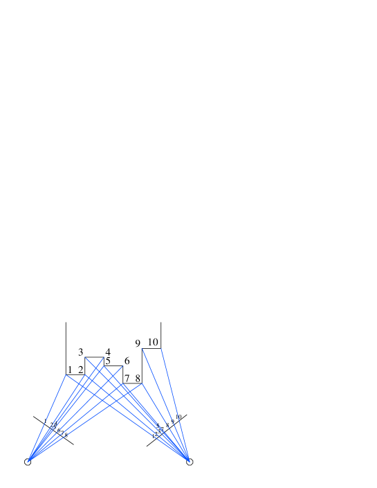

  

  

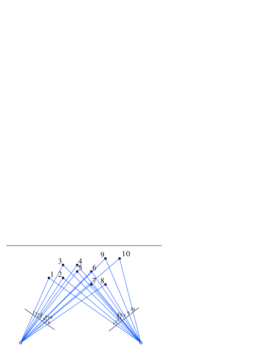
  Figure 4: Illustration of the ordering constraint in classical stereoscopy. The top sketch shows an epipolar plane intersected by a piecewise planar surface. The edges and their projection on the stereo images are numbered to keep track of the viewing perspective. The bottom sketch shows the epipolar plane if the edges were replaced by isolated loops intersecting the epipolar plane.

• Ordering vs. completeness constraint.
  When looking at a continuous, intransparent surface from different view-points, the order at which, e.g., edges are seen in any image along an epipolar line is unchanged. It may happen though that an edge is not visible at all because it is hidden from one of the view points. Fig. 4a illustrates this ordering invariance. Any set of correspondences established between the projections of the edges has to obey this rule and it often strongly constrains the possible correspondences. For the coronal loops and plasma striations, which are optically thin and transparent, this ordering constraint cannot be applied. Instead, if the stereo base angle is not small, the order at which loops are seen along an epipolar line may be permuted (see Fig. 4b). To some extent, the ordering constraint is replaced by a completeness constraint for solar EUV and coronagraph stereo images. In principle, no loop or plasma striation should be lost in the images and any object we see in one image should have a correspondence in the other image. There are practical limitations, however, to this completeness constraint. Some features may lie on top of each other, may be lost if they are faint or are hidden behind the solar disk if they are located at the edge of the solar surface overlap region of the two STEREO spacecrafts.

• Disparity limitation.
  For the objects we observe in solar and coronal stereo images we have a least a rough idea where they are (or better, where they are not) located: not below the solar surface and often we can also give an approximate upper limit for the height above the surface. This valid height range for an object directly transforms into an allowed disparity range. Hence, when searching for a correspondence for a feature in one image, the coordinate range along the epipolar axis of the corresponding feature in the other image is limited accordingly.

• Disparity continuity constraint.
  A smoothly varying depth should yield a smoothly varying disparity both along epipolar lines and on neighbouring epipolar surfaces. If applicable, this constraint could favour certain local correspondences if those in the neighbourhood were firmly established. As mentioned above, this rule is not useful for the loops and plumes we observe in the solar corona. We expect, however, that the three-dimensional curves which represent the location of these objects vary smoothly. Therefore the continuity constraint can be expected to hold at least in the one direction along the curve projections.

2) Similarity measures:

• 

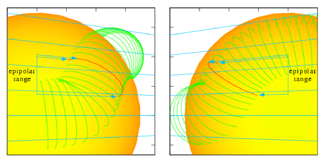
  Figure 5: Identifying loops by their epipolar range. The epipolar lines (light blue) intersected by a particular loop must be identical in both images.

• Common epipolar range.
  Not only must corresponding features be located on the same epipolar line, but if they are part of a projection from, e.g., the same loop, the whole loop must cover the same epipolar range in both images. Since the visible ends of loops often fade out, it may not always be possible to precisely determine its epipolar range. Yet, a comparison of the observed smallest and largest epipolar line value covered by a loop or plume projection including error ranges could help to distinguish loop projections as sketched in Fig. 5. Even more, if a loop projection covers a certain epipolar range twice or more in one image, its projection in the other image must exhibit the same multiplicity in the same epipolar ranges. In properly rectified images this comparison of epipolar coverage is particularly straight forward.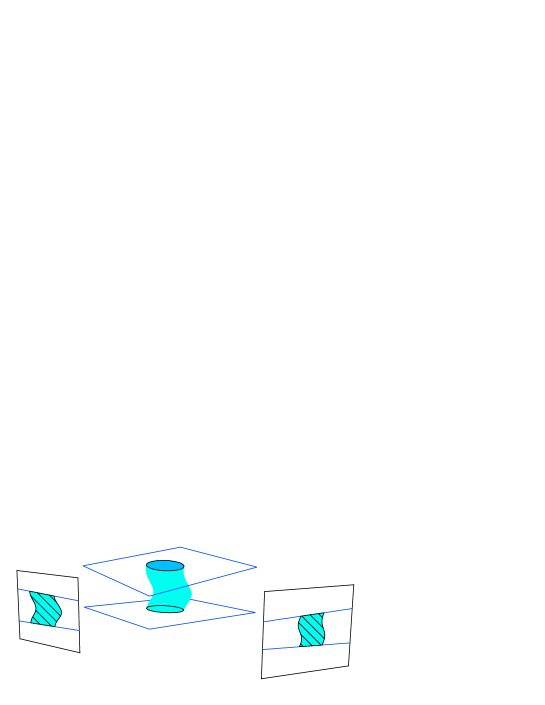

  
  

  Figure 6: Illustration of the integral intensity preservation.

• Integral brightness invariance.
  If the emission from the coronal plasma striations is isotropic, the integrated brightness of a projected loop section (with background subtracted) between two epipolar lines should correspond to the total emissivity of the three-dimensional loop section between the respective epipolar planes and hence should be the same in both images (see the related Helgason-Ludwig consistency condition in tomography, e.g., Natterer (1986, p. 36)). This rule is immediately obvious if we calculate the image intensity by appropriate line-of-sight integrals through the emitting volume as displayed in Fig. 6. The rule holds independent of the inclination the loops with respect to the epipolar planes. But it only holds if epipolar planes are chosen as loop section boundaries: any other boundary plane is viewed differently from the two observers. The integrated brightness of loop intersections along an epipolar line evaluated in both stereo images can therefore effectively help to find the most probable correspondence between the intersections in the two images. A prerequisite for an application of this rule are well calibrated images and instruments with similar signal to noise ratio. The STEREO mission should provide them. A crucial point may be the continuity of the background radiation which has to be subtracted from the integrated loop section intensity. The similarity measure should therefore allow for small deviations of the integrated brightnesses of the order of the background intensity.

More rules can be derived from combinations of different items of the above list: E.g., from the disparity continuity along a loop and the criteria which lead to the disparity limitation we can conclude: If the branch (see section 6 for a precise definition) of a reconstructed loop includes a part which reaches below the solar surface, we can identify the whole branch as a ghost and reject it.

The above list needs to be extended. We are convinced that the reconstructed loop’s consistency with magnetic field models will also lead to helpful similarity measures between loop projections. Since this approach requires the incorporation of additional observations besides the image data, we discuss details of this approach in a separate section 8 below.

The permutation of objects along the epipolar line if viewed from different directions (Fig. 4b) obviously increases with increasing stereo base angle – one reason why the matching is easier for small stereo base angles and why small base angles are often considered particularly favourable for stereoscopy. For the STEREO mission is also important to keep in mind that with increasing stereo base angle the overlapping part of the solar surface is reduced. We will see below, however, that the reconstruction error is much larger for small base angles. Therefore the question for the optimum base angle is difficult to answer. It depends on the one hand on the complexity of the objects which make matching difficult and on the other hand on the desired precision of reconstruction. For the STEREO mission the whole range of base angles beyond 10 degrees will be scanned with time and we will have the chance to test our schemes for practically all angles.

4 Tie-point reconstruction

As we learned above, we can reduce the reconstruction problem to a set of two-dimensional problems. We segment each image densely into a (large) number of epipolar lines and compare the positions of a loop’s intersections along the respective epipolar line in each image. In this section we show how we can derive from these positions the intersection of the loop on the respective epipolar planes.

Figure 7: Reconstruction of a point $\Delta\vec{r}$ with projective (top) and affine (bottom) geometry.

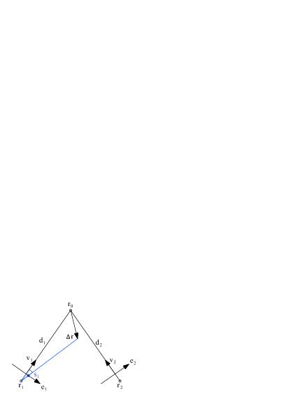
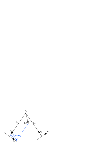
Let on a given epipolar plane the observer’s positions be $\vec{r}_{1}$ and $\vec{r}_{2}$. For each epipolar plane we in addition specify a reference point $\vec{r}_{0}$ as the origin of the two-dimensional coordinate system on this plane. For convenience, we could take the intersection of the solar rotation axis with the epipolar plane the intercept of which could at the same time serve as a continuous label for the epipolar plane. For each observer we then introduce orthogonal coordinate axes $\vec{v}_{i}$ and $\vec{e}_{i}$ on the epipolar plane as shown in Fig. 7: $\vec{v}_{i}$ is the unit vector from the observer to $\vec{r}_{0}$ and $\vec{e}_{i}$ is $\vec{v}_{i}$ rotated clockwise by 90 degrees. Note that $\vec{v}_{i}$ do not need to agree with the optical axis of the telescope nor must $\vec{e}_{i}$ have the direction of the epipolar line.

Figure 8: Derivation of the angle $s$ from the image coordinates for a projective geometry camera model.

We will take as rectified image coordinate along the respective epipolar line in image $i$ the angle $s_{i}$ between the direction to the object and $\vec{v}_{i}$. For convenience, we assume that the mapping of the observing telescopes can be described by a simple projective geometry camera model. In this case, an object at an angular distance $\sigma$ from the optical axis is mapped in the image to a distance $\rho$ = $f\tan\sigma$ where $f$ is the camera’s focal length. In this case, the angle $s_{i}$ can be derived from the image distances $\rho_{0}$ and $\rho$ of the reference and object point’s projection from the image centre, respectively, and their azimuth difference $\gamma$ (see Fig. 8) by

$$\cos s_{i}=\frac{f^{2}+\rho_{0}\rho\cos\gamma}{\sqrt{f^{2}+\rho_{0}^{2}}\sqrt{f^{2}+\rho^{2}}}$$ (1)

Here, the sign of $s_{i}$ depends on whether the object is projected to the right(+) or left(-) of the line from the image centre to $\vec{r}_{0}$’s projection. If there is any image distortion, the distances $\rho_{0}$ and $\rho$ read from the image have to be corrected accordingly. Formula (1) is numerically inconvenient for large focal lengths $f$ and small image distances $\rho$. For $\rho/f$, $\rho_{0}/f$ $\rightarrow$ 0 relation (1) can be approximated by

$$s_{i}^{2}=(\frac{\rho_{0}}{f})^{2}+(\frac{\rho}{f})^{2}-2\frac{\rho_{0}\rho}{f^{2}}\cos\gamma+\mathcal{O}\big{(}(\frac{\rho}{f})^{4}\big{)}$$ (2)

which is the law of cosines applied to the triangle in the image plane in Fig. 8. Hence, the angle $s$ can in this limit be read directly from the image in units of arcsecs.

The necessary camera calibration information is then contained in the position of the observers $\vec{r}_{i}$ and either the reference point $\vec{r}_{0}$ or the two view directions $\vec{v}_{i}$ to the reference point. In the latter case, $\vec{r}_{0}$ can be determined from (see Fig. 7a)

$$\vec{r}_{0}=\vec{r}_{1}+d_{1}\vec{v}_{1}=\vec{r}_{2}+d_{2}\vec{v}_{2}$$ (3)

$$(\vec{v}_{1},\vec{v}_{2})\left(\begin{array}[]{c}\!\!d_{1}\!\!\\ \!\!-d_{2}\!\!\end{array}\right)=\vec{r}_{2}-\vec{r}_{1}$$ (6)

Therefore a rectified image point $(s_{1},s_{2})$ = (0,0) will have to be reconstructed at $\vec{r}_{0}$ and any other $(s_{1},s_{2})$ pair will be conveniently expressed as a two-dimensional distance vector $\Delta\vec{r}$ from $\vec{r}_{0}$.

For affine geometry, all view directions from an image $i$ are approximated to be parallel to $\vec{v}_{i}$. Then (see Fig. 7b)

$$\left(\begin{array}[]{c}\!\!\vec{e}_{1}^{T}\!\!\\ \!\!\vec{e}_{2}^{T}\!\!\end{array}\right)\Delta\vec{r}=\left(\begin{array}[]{c}\!\!d_{1}\tan s_{1}\!\!\\ \!\!d_{2}\tan s_{2}\!\!\end{array}\right)$$ (7)

If we subtract the two above lines we obtain the “depth” component of $\Delta\vec{r}$ in direction half way between the two view directions. Note, with $beta$ the angle between $\vec{v}_{1}$ and $\vec{v}_{2}$ we have $\vec{v}_{1}+\vec{v}_{2}$ = $(\vec{e}_{2}-\vec{e}_{1})/\tan(\beta/2)$. Then

$$\tan\frac{\beta}{2}\;(\vec{v}_{1}^{T}+\vec{v}_{2}^{T})\Delta\vec{r}=d_{1}\tan s_{1}-d_{2}\tan s_{2}$$ (8)

where the difference on the right hand side is the disparity. In the simplest case, the depth of an object is directly proportional to the disparity of its projections along the epipolar lines.

For projective geometry we take account of the divergence of the view directions emerging from each observer. The angle $s_{i}$ between the reference point $\vec{r}_{0}$ and an object in the epipolar plane then is (see Fig. 7a)

$$\tan s_{i}=\frac{\vec{e}_{i}^{T}\Delta\vec{r}}{d_{i}+\vec{v_{i}}^{T}\Delta\vec{r}}$$

or

$$\left(\begin{array}[]{c}\!\!\vec{e}_{1}^{T}-\vec{v}_{1}^{T}\tan s_{1}\!\!\\ \!\!\vec{e}_{2}^{T}-\vec{v}_{2}^{T}\tan s_{2}\!\!\end{array}\right)\Delta\vec{r}=\left(\begin{array}[]{c}\!\!d_{1}\tan s_{1}\!\!\\ \!\!d_{2}\tan s_{2}\!\!\end{array}\right)$$ (9)

in contrast to (7). To justify the more simple affine geometry formula, $s_{1}$ and $s_{2}$ must both be small. For EUVI images, $s$ is of the order of the the apparent solar disk radius of about 0.005 radian. For HI images, however, with a much larger field of view, projective geometry is unavoidable. Even if $s$ is small some care is necessary, because in (7), the matrix on the left has to be inverted and small changes in its parameters may alter its minor eigenvalue considerably. The eigenvalue of a matrix $(\vec{a},\vec{b})$ is $\mathcal{O}(\lvert\vec{a}\times\vec{b}\rvert)$ if it is small compared to $\lvert\vec{a}\rvert$ and $\lvert\vec{b}\rvert$. Hence if the view directions are nearly parallel, the difference between affine and projective geometry may be non-negligible even if $s$ is small.

Figure 9: Reconstruction of a curve segment (red) with different inclination with respect to the adjacent epipolar planes (blue). In the top drawing the line segment in inclined to, in the bottom drawing it lies exactly on an epipolar plane. (bottom).

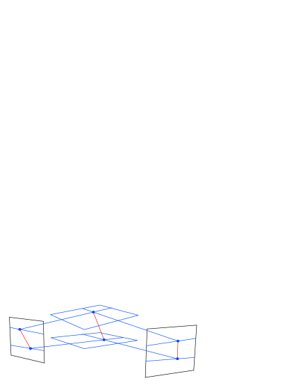
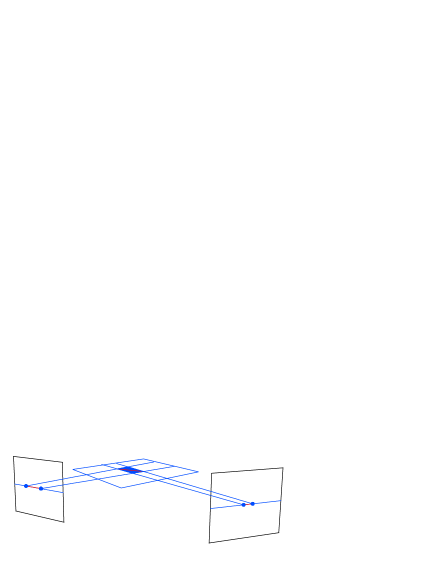
For each epipolar plane we obtain a set of intersection points and all we have to do is to connect the intersection points between neighbouring planes to obtain three-dimensional curves. This last step involves some uncertainties if different loops come close. To obey the disparity continuity constraint we should keep track of the intersections across the epipolar planes by reconstructing curve segments between epipolar lines rather than only points on single epipolar lines (Practically, we just combine the intersection points of a given curve projection with epipolar lines to ordered lists). Hence the method should better be called tie-curve rather than tie-point method.

The curve segments from each image are then projected along their respective geometrical view direction (either affine or projective) which yields a narrow planar strip of the projection surface of the curve (see Fig. 9a). The intersection of the strips from both images gives a small line segment of finite length, the end points of which are two points of the three-dimensional loop curve. The intersection is guaranteed since the curve sections in the image were chosen from the same epipolar interval.

This strategy runs into a problem, however, if the curve segment is directed parallel to an epipolar line (see Fig. 9b). The geometrical intersection of the two projection ribbons now is not a line segment anymore but a small trapezoid. This object of dimension 2 is difficult to incorporate to our final three-dimensional loop curve of dimension 1. This problem, however, is not a deficit of the method but a fundamental geometrical limitation which will be addressed in the following sections. It is a hint that the reconstruction error at this point of the loop becomes singular and in general, this is the point where the true solution for the loop curve may intersects with ghost features.

5 Reconstruction errors

Figure 10: Local orthogonal coordinate system along the reconstructed loop (in red) used to express the uncertainty area (red dashed square) at a point along the loop. The position uncertainty in direction $\vec{n}$ is given by the resolution $w$ of the image. The precise position of the curve in direction $\vec{n}\times\vec{t}$ can only be determined by the resolution of the second image. The projection surface of this second image is not shown for clarity, it intersects the projection surface from the first image (blue) along the red loop curve.

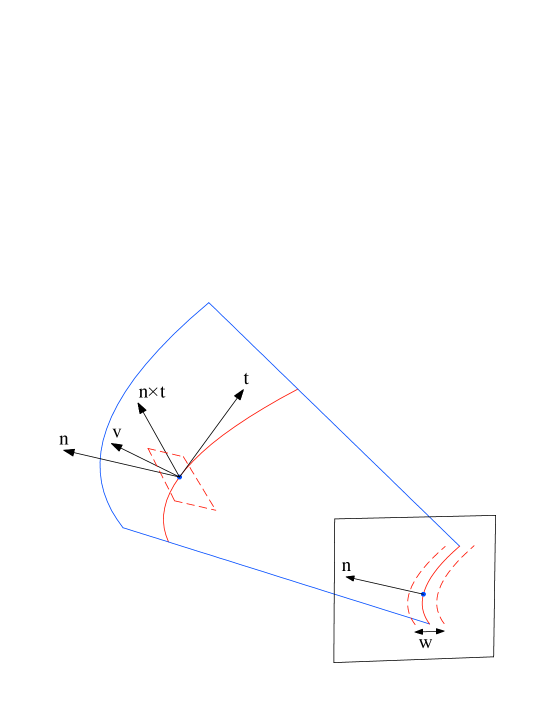
If a loop’s projection in an image can only be determined with a finite resolution, there remains a positional uncertainty of the final three-dimensional curve. Consequently, we have to think of the projection surfaces as surfaces of finite thickness and their intersection yields a tube with trapezoidal cross section within which the final curve position cannot be resolved. The reconstruction uncertainty of a single point along the three-dimensional curve due to the finite width $w_{i}$ of the loop in image $i$ lies in the plane spanned by the local normals $\vec{n}_{i}$ of the two projection surfaces at the point where the projection surfaces intersect (see Fig. 10). Hence the positional uncertainty is distributed normal to the local loop tangent $\vec{t}=\vec{n}_{1}\times\vec{n}_{2}/|\vec{n}_{1}\times\vec{n}_{2}|$ as should be because uncertainties along the loop are irrelevant.

This error trapezoid at any point $\vec{r}$ along the loop can be expressed as

$$\delta\vec{r}=\pm a_{1}\vec{t}\times\vec{n}_{1}\pm a_{2}\vec{t}\times\vec{n}_{2}$$ (10)

where the $a_{i}$ are to be determined so that the projection of the trapezoid onto image 1 and 2 yields the right loop width $w_{1}$ and $w_{2}$, respectively. Upon multiplying (10) with $\vec{n}_{1}$ and $\vec{n}_{2}$ we obtain

$$a_{1}=\frac{w_{2}}{2\sin\alpha}\quad\text{and}\quad a_{2}=\frac{w_{1}}{2\sin\alpha}$$ (11)

where $\lvert\vec{n}_{1}\times\vec{n}_{2}\rvert$ = $\sin\alpha$ and $\alpha$ is the angle between the local projection surface normals.

Figure 11: Error trapezoid in the plane normal to the loop. The loop’s tangent $\vec{t}$ points out of the plane and $\alpha$ is the angle between $\vec{n}_{1}$ and $\vec{n}_{2}$.

If $w_{1}=w_{2}=w$ we have a local trapezoid with main axis length (see Fig. 11)

$$\frac{w}{2\sin\alpha}\vec{t}\times(\vec{n}_{1}\pm\vec{n}_{2})$$ (12)

where the length of $(\vec{n}_{1}\pm\vec{n}_{2})$ is $\cos(\alpha/2)$ and $\sin(\alpha/2)$, respectively. The axis lengths of the error trapezoid are therefore (measured from the centre to the trapezoid corners)

$$\frac{w}{2\cos(\frac{\alpha}{2})}\quad\text{and}\quad\frac{w}{2\sin(\frac{\alpha}{2})}$$ (13)

We note, that the positional error with which we can reconstruct a loop from finite resolution images does not depend on the stereo base angle between the view directions $\vec{v}_{i}$ of the two observers but rather on the angle $\alpha$ of the projection surfaces.

The two angles are not independent, though. $\alpha$ is always smaller or at best equal to the stereo base angle. Where the loop tangent $\vec{t}$ intersects an epipolar plane in normal direction, the normals $\vec{n}_{i}$ are just the $\vec{v}_{i}$ rotated by 90 degrees. In this case, $\alpha$ is identical to the stereo base angle. If, however, the loop tangent lies in the intersected epipolar plane (the situation sketched in Fig. 9b), the $\vec{n}_{i}$ are both the epipolar plane normal, hence are parallel and $\alpha$ = 0 whatever the stereo base angle.

We have seen already in the previous section about the tie-point reconstruction that we encounter a problem where the loop’s images are directed parallel to the epipolar lines. This complies with our error estimate which becomes singular in this case.

If, as at the beginning of the STEREO mission, the stereo base angle between the two observing spacecrafts is small, (13) poses a severe restriction to the resolution with which we can reconstruct the loops. For a stereo base angle of 10 degrees, we have $\alpha$ $\leq$ 10^∘ and with $w$ set to the resolution of the STEREO EUVI images of 2 arcsec, (13) gives $\pm$8000 km. Hence the resolution in the direction half way between the two view directions ($\vec{n}_{i}\times\vec{t}$ is the view direction mapped to the plane normal to $\vec{t}$) will not be better than about 16000 km in vertical direction on the solar surface. The resolution will, however, rapidly improve while the STEREO spacecrafts separate. The error can also be reduced if the position of the loop in the image can be determined with subpixel precision by a suitable interpolation of the image intensities in the vicinity of the loop projection.

In general, the numerically reconstructed loop curve will stochastically vary within the above estimated error range due to small fluctuations in the detected loop projection and numerical round-off effects. Especially if the stereo base is small, the resulting three dimensional curve may look very different from what we expect to be a magnetic field line. A coronal magnetic field line should show a smooth change of the local curvature vector $d\vec{t}/d\ell$ (see Frenet’s formulas, $\vec{t}$ is the unit tangent and $\ell$ the length coordinate along the loop). One way to improve the tie-point method would be to not only reconstruct the curve, but along with it store the local error axes and their length estimates for every loop point. In a post-processing step the three-dimensional curve is then smoothed (e.g., by a smoothing spline) within these error bounds so that the variation of the curvature vector along the loop is minimized. In its extremes, this approach leads to loop curves with constant curvature, i.e., sections of circles as proposed by Aschwanden et al. (1999).

Figure 12: EIT observations of an active region taken 23 hours apart In white we show the attempts to trace out a loop which is well visible in the contrast enhanced image.

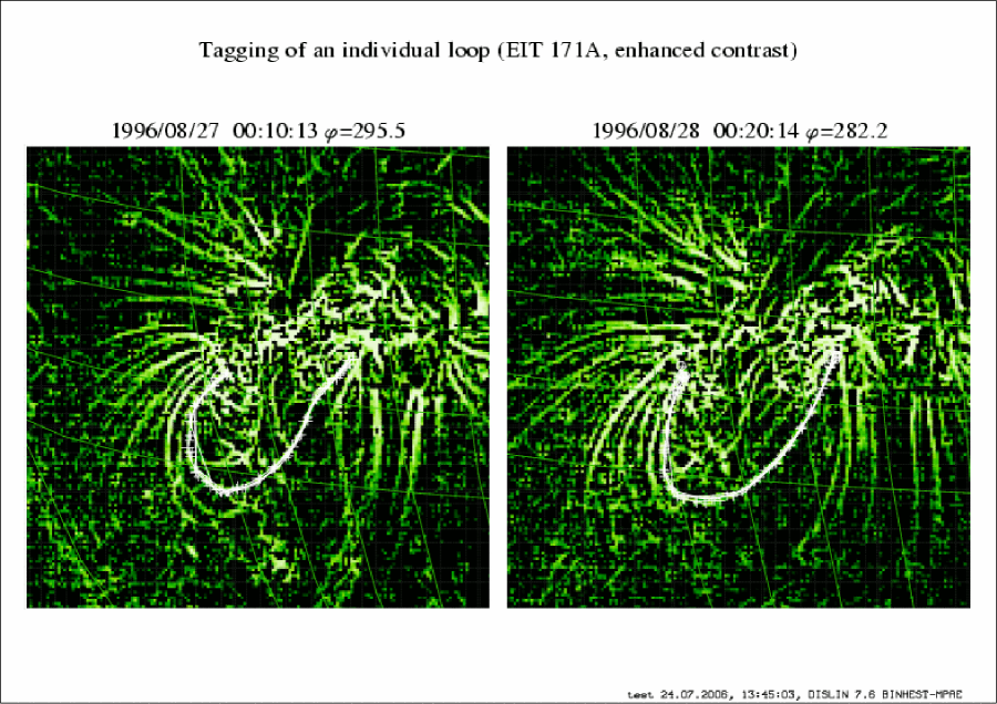
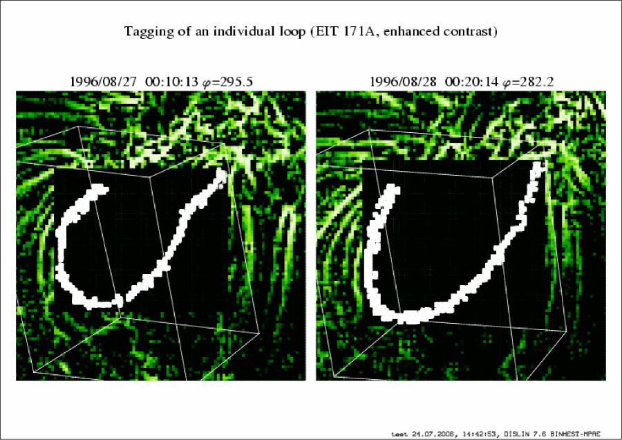
As an example, we show the reconstruction attempts for a single field line of an active region from a pair of EIT observations in Figs. 12 and 13. Due to the present lack of true STEREO data, two images were selected which were taken approximately 23 hours apart. The solar rotation then produces an equivalent stereo base angle of 12.8 degrees. To make the loop structures better visible, the images were contrast enhanced with an filter of even order (Note that filters of odd order such as Sobel are less noisy but may shift the intensity enhancement away from the loop centre).

Figure 13: Results of the reconstruction (blue) from the loop projections shown in Fig. 12 viewed at from two different directions which do not coincide with the view directions of the observations. The solar surface is indicted by a latitude/longitude grid (red) and the loop projections are mapped as green curves onto the solar surface.

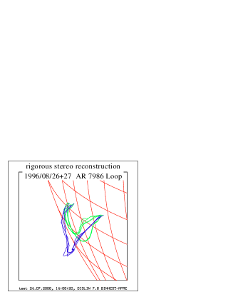
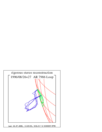
Fig. 12 displays the manually traced loop projections on top of the respective EIT image while Fig. 13 shows the reconstruction from the loop projections. The reconstructed loops are displayed from two view points, each different from the observing directions. The second of these views which shows the reconstructed loop just above the limb reveals the substantial variation of the reconstructed curve in vertical direction, approximately the view directions of the two observations. This insensitivity of the reconstruction in height is a consequence of the small stereo base angle as discussed above. Besides this large vertical error, the loop very probably also has slightly changed its shape in the time interval between the observations of image 1 and 2 which might also add to its odd appearance. This can somewhat be guessed from the kinks in the loop projection of image 1 which are absent in image 2.

Figure 14: A circle and a torus fitted to the observations.

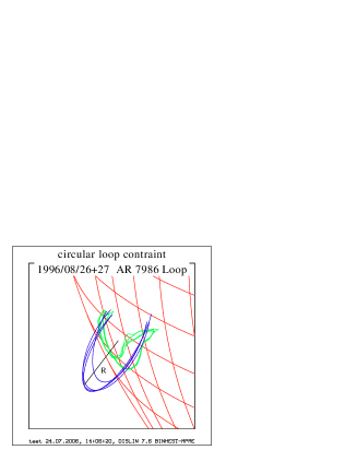
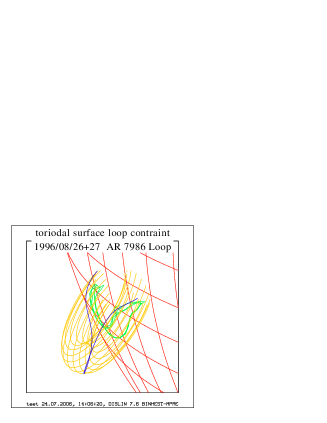
Finally, Fig. 14 shows the attempt to force the loop into a shape with a small variation of the curvature vector. The loop was fitted to a circle of constant radius (left) and to the surface of a torus of constant major and minor radii (right). These approaches have been suggested by Aschwanden et al. (1999); Aschwanden (2005).

From the forthcoming STEREO mission, we hope to obtain image data which has better resolution than the EIT data so that such an extreme smoothing of the reconstructed curves will not be necessary.

6 Ambiguities

One source of ambiguous reconstruction results is our limited ability to make definite correspondences between loop projections. Every alternative correspondence produces a new individual loop or possibly even a whole set of new loops. If the constraints listed in section 3) do not help us to discard multiple correspondences, the image data alone cannot be interpreted in an unambiguous way.

Figure 15: Double solutions obtained from the reconstruction of a single arc. In each image, the projection covers a certain epipolar range twice with a turning point in between.

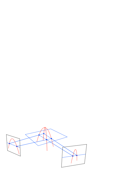
Even individual loops can fool us. The simplest example is a magnetic arc (Fig. 15) which, if viewed from two different directions can be interpreted in two ways represented by the two crossing arcs. A typical feature of these ambiguous reconstructions is that they intersect exactly at an epipolar turning point where the loop projections become parallel to the epipolar line. We recall that this is a critical point in the reconstruction anyway because the reconstruction error becomes singular at this point.

Figure 16: Apparent field line reconnection obtained from the reconstruction of a single magnetic arc where one of the projections was erroneously shifted upwards (top) and downwards (bottom). The projection in light red in the right image indicates the original position.

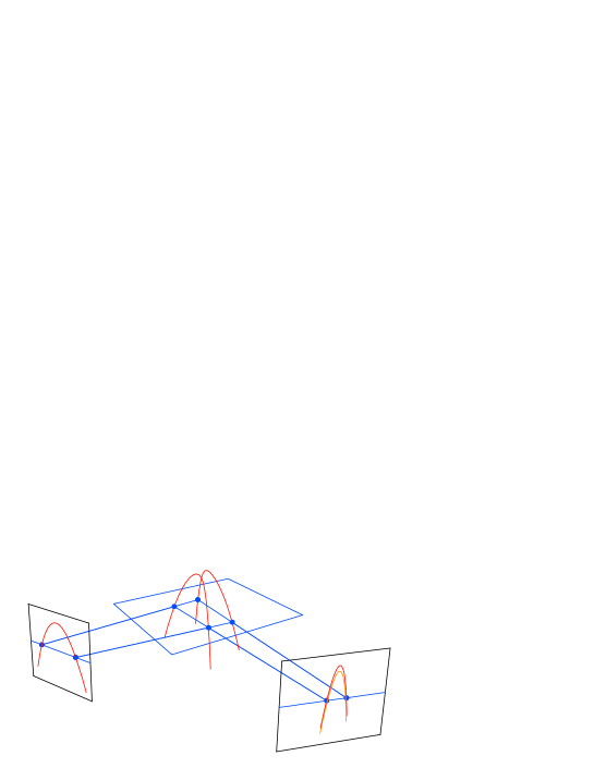
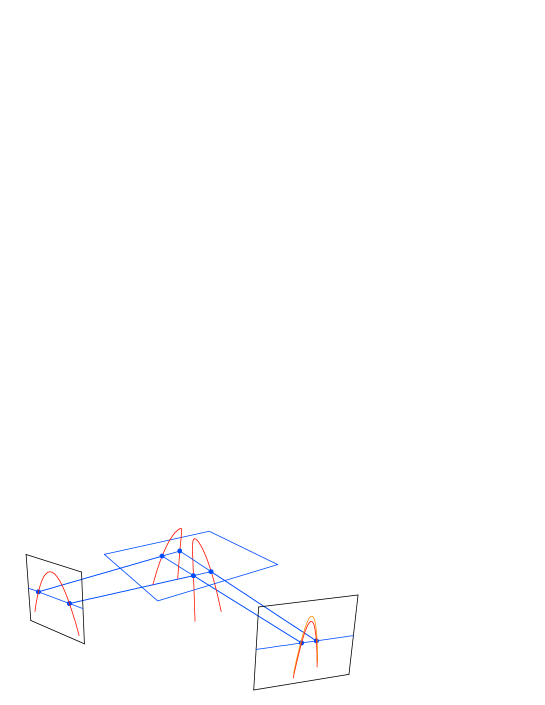
This is in particular demonstrated if we add little errors to one or both of the loop projections as in Fig. 16. Here, the projection in the right image was shifted up- and downwards by a small amount. The crossing arcs split in a characteristic way with the deviations from the original solution being biggest at the top of the arc. Both observations if made in sequence would appear as if we had observed field line reconnection and yet it’s only a combination of finite measurement errors and stereoscopic ambiguity.

In the following we will define the reconstructed curve sections, which due to small errors may connect with each other in different ways as curve branches. Since the reconnections obviously occur at the epipolar turning points, each branch consists of a curve section with a monotonously varying epipolar coordinate along the curve.

With a finite image resolution included, it may well occur, that a branch of the true reconstruction solution combines smoothly with a ghost branch. This phenomenon may make a distinction between true and ghost branches particularly difficult. These false connections, however, can only occur where the loop projections are directed parallel to the epipolar lines. This condition may help to concentrate post-processing checks of the reconstructed loops on these critical points.

Common to the above examples in Figs. 15 and 16 is that the loop projections in both images cover a certain epipolar range twice with the critical epipolar turning point right in between. We find from the reconstruction four branches each monotonous in the epipolar coordinate. This principle can fairly easily be generalized: a loop projection, which crosses a certain epipolar line $n$ times should only match with a projection in the other image which also intersects this epipolar line $n$ times (intersections which fall on top of each other are counted with according multiplicity). If this extends over a finite epipolar range, the rigorous reconstruction yields $n\times n$ branches, some of which may connect at the boundaries of the epipolar range if a turning point in the loop projection is present at the respective epipolar line.

Figure 17: Multiple solutions for the reconstruction of a loop which covers a certain epipolar range three times.

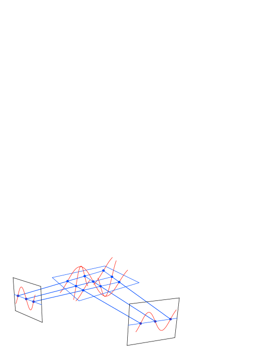
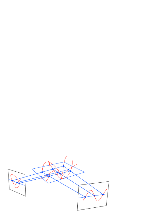
We demonstrate this principle in Fig. 17 with a threefold coverage of a certain epipolar range by the loop projections. We see that nine branches can be reconstructed, each monotonous in the epipolar coordinate. Two of these remain isolated, four more connect pairwise and only the remaining four connect to a continuous curve which produces the full loop projection. Hence if we expect the true solution to form a single continuous loop, this last one has to be the right solution and all other branches are ghost features.

Figure 18: Typical closed loop ghost features which result if the curves projections in each image has extrema at different epipolar values.

So far we have assumed that we have found the right pair of projections originating from one loop. We may erroneously make a wrong correspondence and try to reconstruct from projections which do not belong to the same original loop. Typical reconstruction branches which may result from such an attempt are shown in Fig. 18. We see isolated branches and branches connected at both ends so that they form a closed curve. None of the connected branches covers the entire projection in both images. This may be taken as a hint that the two projections do not make a valid correspondence.

Figure 19: A stereo image pair with groups of loops which have a different number of intersections with epipolar lines. Conjugate pairs of epipolar lines are superimposed on each image.

Figure 20: Reconstruction for one of the group of loops of Fig. 20. The reconstructed curves are drawn in red, except for those parts which lie inside the Sun and which are drawn in light red.

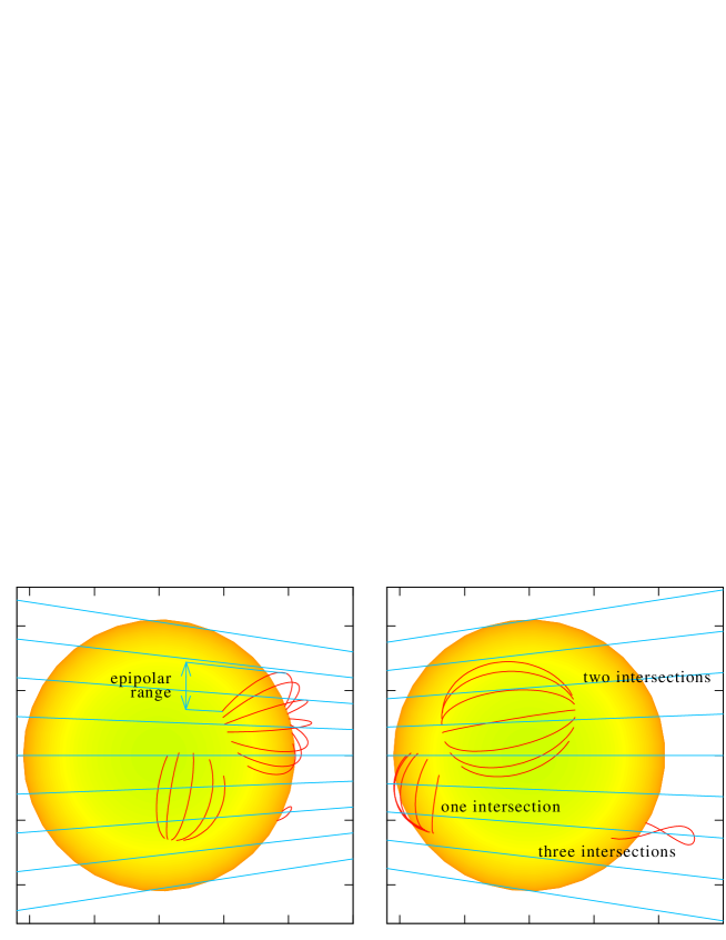
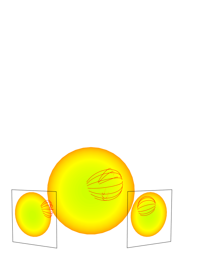
Fig. 20 summarizes our findings. Since epipolar lines for the STEREO mission are only slightly inclined with respect to the ecliptic, loops in north-south direction are straight forward to reconstruct once they have been identified in both images. An example is the arcade on the southern hemisphere in Fig. 20.

Loops with east-west orientation usually intersect some epipolar lines twice if they are curved. The example here is the set of loops in the northern hemisphere in Fig. 20. The only exception is the loop at the centre of this group. We have to expect therefore that the reconstruction of these loops is ambiguous and yields two crossing arcs each. Since the individual loops do not cover a large epipolar range we can even anticipate that the pair of reconstructed arcs makes only a small angle with each other and may be difficult to distinguish. Fig. 20 shows the result of the reconstruction of these loops. In fact, for the reconstruction of the central loop which is the only unique one, the pair of arcs coalesces to a single arc. Unfortunately these more complicated east-west orientated loops are far more common for active regions on the solar surface.

Less common and even harder to reconstruct are loops with triple crossings of an epipolar line as indicated by the individual loop above the southern limb in the right image. In this case a reconstruction is impossible anyway because the loop is hidden behind the solar limb in the left image.

7 More than two viewpoints

We learned above that the epipolar geometry is especially adapted to an image pair. A third or even more images are difficult to include directly unless certain simplifying assumptions concerning the overall geometry are made. The simplest way to make use of additional (simultaneous) images is to produce stereo reconstructions from pairwise combinations of the images. Since the ghost features very probably will be located differently in the reconstructions from different image combinations, the intersection of all reconstruction models should eliminate most of the ghosts.

Figure 21: Stereo reconstructions of a CME-like extended flux rope (red) including ghost features (light red). The top panel shows the reconstruction based on two stereo images, the bottom panel the reconstruction from three simultaneous images taken all from the ecliptic plane.

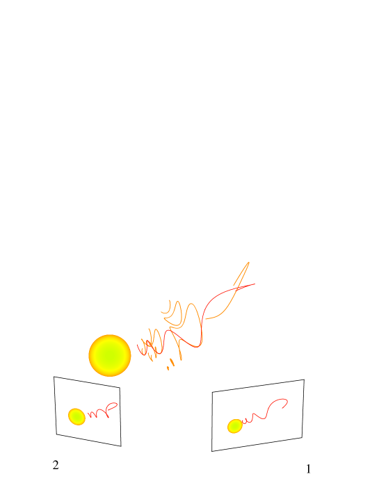
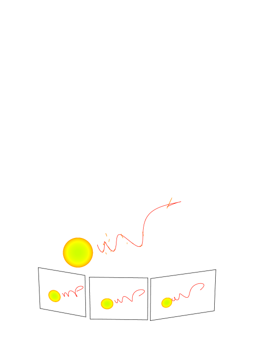
In order to demonstrate the advantage of a third view we consider a more extended and more complex object as above. Fig. 21 shows a very simplified model of a CME flux-rope. The original field line curve is drawn in red and it is faithfully reconstructed. However along with it the reconstruction includes a number of ghost features drawn in light red in the top of Fig. 21. We recognize the isolated curve branches and closed field line curves typical for ghost features as in Fig. 18. In the magnetic cloud of a CME closed field lines of such shape very probably do not occur.

If we include a third view in the reconstruction, e.g., from a near-earth position, we can produce three reconstruction models which, if properly done, all include the true field line curve. The ghost features from the different reconstructions on the other hand hardly overlap and can thus be almost completely eliminated except for a few short line segments which are easily recognized as false in the bottom diagram of Fig. 21.

For the STEREO mission, the “third eye” could be provided by ground based coronagraphs or by the SOHO/EIT and LASCO instruments. All three observers would then be placed in the ecliptic at almost equal angular distance to its neighbour. An even more advantageous arrangement would be a third spacecraft out of the ecliptic. In this case the mutual epipolar plane systems would make a large angle with respect to each other. In this geometry, critical reconstruction points where loop tangents are parallel to the epipolar lines in one epipolar system would be regular reconstruction points in the other systems and reconstruction errors could be effectively reduced. For the arrangement as shown in the lower part Fig. 21, the critical reconstruction points stay close together in all three epipolar systems and the error prone loop sections remain.

The advantage of a third view also only pays if the stereo base angle is large enough. Recalling our error estimates in section 5 the mutual angles between the view directions should be larger than about 10 degrees. Otherwise the geometrical uncertainty may partly be larger than the distance between true and ghost curve features.

8 Magnetic field

The fact that the plasma striations we want to reconstruct are strictly aligned along the magnetic field suggests that we use magnetic field information in addition to the image data to help with the reconstruction.

Figure 22: Observed loop projections (thick) and projected potential field lines (thin) for an active region with a surface normal magnetic field component indicated by the thin contour lines. From Aschwanden et al. (1999).

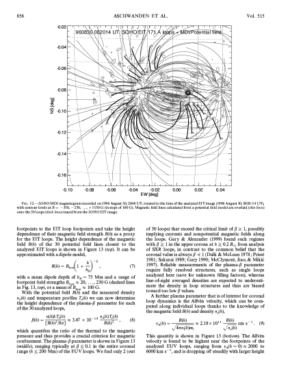
Magnetic field observations are available from solar surface Zeeman and Hanle effect observations. Hardly any direct field measurements have been made in the corona because line intensities there are much fainter, thermal line spread much larger and field magnitudes much less than in the photos- and chromosphere. The coronal field is therefore often deduced from the surface observations by means of field extrapolation. The extrapolation requires assumptions about the the complexity of the field. The simplest and most often used is the assumption that electric currents are absent and that the magnetic field is a Laplace field. Observations show, however, that field lines calculated under this assumption often deviate from observed loops, especially near active regions (see, e.g., Aschwanden et al. (1999) from where we took Fig. 22 and Wiegelmann et al. (2005)).

Figure 23: Stereo image pair with identified loop projections (top). The coloured curves correspond to the projections of close field lines calculated from different magnetic field models which were used to establish the correspondences between the loop projections. A three-dimensional reconstruction of the observed loops includes ghosts if these correspondences are ignored (bottom left). The original model could faithfully be retrieved if they were accounted for (bottom right). From Wiegelmann and Inhester (2006).

More sophisticated field assumptions postulate the vanishing of the Lorentz force which is reasonable for quasistationary field configurations given the dominance of the magnetic field in the corona. These so-called “force-free” field models, however, require the solution of a non-linear boundary value problem. The development of codes which are able to effectively calculate force-free fields from observed boundary is still in progress (Amari et al., 2006; Inhester and Wiegelmann, 2006; Schrijver et al., 2006). A deficit of these models is that they require boundary values to some extent not only on the solar surface where the observations provides them but also on the computationally unavoidable lateral and top boundaries where they have to be guessed. Hence, also the magnetic field models available will not be unique and an intimate combination of stereoscopic reconstruction and magnetic field modelling is probably required to make definite progress.

With this approach in mind, Gary and Alexander (1999) started from a Laplace field extrapolation and suggested to gradually alter this initial magnetic field until the projected field lines match best the observed loop projections. Gary and Alexander considered a mere radial stretching as deformation. The resulting field is no more potential, it is not force-free either because the radial stretching complies with toroidal currents which are not necessarily aligned along the magnetic field. In absence of stereo images, a magnetic field model could be produced which agreed with observed loop projections in one image. The resulting Lorentz force, however, necessary to achieve the agreement by radial field line stretching was considerable.

Lee et al. (2006) proposed to make use of magnetic field information at a very early stage of the image processing when loop projections are traced in the images. As mentioned above, this segmentation of EUV images into curves which trace out the loop projections is an image processing problem of its own, but it is also a prerequisite for the tie-point stereo reconstruction. After a first step of identifying image pixels which lie on the intensity ridge of a projected loop the magnetic field is used to determine the connectivity of these ridge pixels. In their oriented connectivity method, Lee et al. restrict the range of azimuth orientations within which the next ridge pixel is looked for from the range of magnetic field azimuths that project onto the pixel from the Laplace field calculated at various heights above the solar surface.

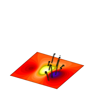
According to an idea of Wiegelmann and Inhester (2006), magnetic field information could be used also to find correct correspondences between loop projections in the stereo images. In a first step, distances between projected loops in the stereo images and field line projections onto these images are calculated. After appropriate ordering of loops and field lines according to this distance those loop projections in the two stereo images are assumed to correspond which are closest to a common field line. The uniqueness constraint was explicitly taken account of in this procedure and different distance norms and field models were tested. However, this idea has so far only been applied to simple synthetic loop models. Fig. 23 shows at the top the projected loops which were simulated from a known force-free magnetic field. The closest field lines are superimposed with a colour code which relates to different field line models used to find the corresponding loops. Even the Laplace field model which can only insufficiently reproduce the correct field still resulted in correct correspondences.

The magnetic field information could also be of help when the reconstructed curve branches are connected across epipolar turning points (see section 6). An estimate of the local magnetic field direction in the vicinity of the turning point serve a measure which connection is the most probable in a similar way as in Lee et al. (2006)’s oriented connectivity method.

9 Stereoscopy by tomography

Figure 24: Assumed distribution of light sources along the projection ray from a bright image pixel in stereoscopy (left) and tomography (right).

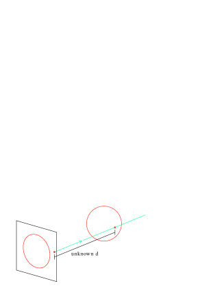
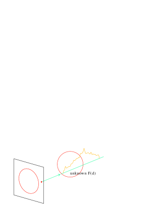
Tomography provides a different approach to three dimensional reconstruction. It differs from stereoscopy by a fundamental assumption: Stereoscopy assumes that the light which illuminates an individual image pixel is concentrated in a single space point while in tomography the light source is assumed to be continuously distributed along the line-of-sight inside a limited domain (see Fig. 24).

Hence with stereoscopy, a second view is sufficient to locate the isolated light source while a large number of additional views are required to determine the continuous emissivity distribution. However, if the source satisfies (more or less) the stereoscopy assumption of locally concentrated light sources, a tomography scheme can still be used because its assumptions are more general.

Figure 25: EIT observations of an active region taken 23 hours apart after contrast enhancement. In white we show the attempts to trace out a loop which is well visible in the contrast enhanced image.

Figure 26: Tomographic reconstruction of a loop from the contrast enhanced data in Fig. 26.

In tomography not only the location but also the intensity of loop projections count and we can in principle hope to obtain a quantitative emissivity distribution along the loop. The handicap of tomography is, however, that it needs a larger set of view directions to resolve the emissivity distribution. For the solar corona this can only be obtained by exploiting the Sun’s rotation and assuming stationarity of the observed structures.

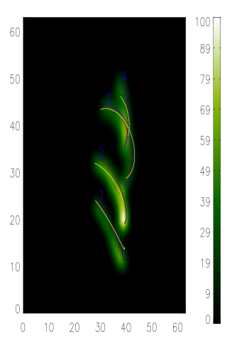
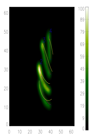
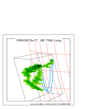
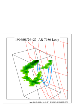
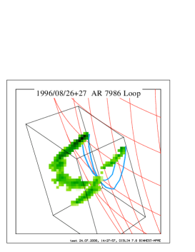
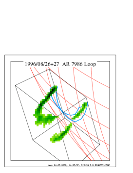
In Fig. 26 and 26 we show an example where we have tried to compromize between the additional requirements and the additional output of tomography with respect to stereoscopy. The intensity information is abandoned, the images are strongly contrast enhanced and the background is thresholded to a nearly black/white image.

The two stereo images were subsequently used as input for a tomography inversion code. The zero background intensity after thresholding makes this data ideal for a multiplicative inversion algorithms. We have used a Richardson-Lucy algorithm (RLA, see, e.g., Lantéri et al. (1999), for alternatives see, e.g., Byrne (1998)) to produce the results shown in Fig. 26.

The original data is the same as for the tie-point reconstruction shown in Fig. 12. Similar to this above example, our results here suffer from the same deficiency: the small stereo base angle yields a large uncertainty of the loop position in vertical direction which in Fig. 26 is visible by the relatively large spread of the loop model in vertical direction.

It is also obvious that the tomography code just as the stereo reconstruction is unable to distinguish between true and ghost branches and some post-processing of the tomography results will in general be necessary. An advantage of the multiplicative algorithm we have used above is that it converges after few iterations. If ghost branches can then be identified in the resulting preliminary model distribution they just need to be wiped out by setting the respective voxels to zero. Resuming the iterations subsequently will redistribute the uncompensated image intensities onto the remaining branches and the eliminated ghosts will not reappear. Another advantage of the tomography approach is that it can without conceptual extensions cope with more than two images. All the geometrical constraints which we must explicitly take care of in stereoscopy are hidden in the sparse forward matrix which needs to be inverted for tomography. This matrix grows, however, with every additional image.

Tie-point code example

Stereoscopic reconstruction is in a way an inverse problem. Working on problems of this kind requires some theoretical background part of which we have tried to convey with this paper. A more concise account of the geometrical principles of stereoscopy can be found in (Faugeras and Luong, 2001). On the other hand, own experience is also indispensable when applying your knowledge to a specific inverse problem. A review on modelling and reconstruction attempts with solar physics data has been recently compiled by (Aschwanden and many more, 2006). To enable the reader to make an own first step also in this direction, we supply a simple tie-point code along with this paper. It can be ordered as free software from the author (email: binhestmps.mpg.de). You will recieve a file stereo_02.tar.gz which has to be unpacked in the usual way. Installation instructions are given in the contained readme file. You further need a FORTRAN90/95 compiler and, if you want to see the graphics output, the free DISLIN graphics library from www.dislin.de.

If you make it, you produce an executable named stereo. This program reads observer parameters and 3D curve data from the file stereo.dat. The image projection is made in subroutine xc2pxc, the image rectification in pxc2epi and the reconstruction in epi2xc. The program can be run without graphics if you do not have DISLIN. In this case you need to comment the graphics calls in the source text in stereo.f90 accordingly and remake.

If you use the graphics, the original curve xc and its projections are drawn in red, the reconstructed curve branches xb in yellow (the original xc should no more be visible). A left mouse click relative to the cross in the image centre defines the direction into which the main observer is to move for the subsequent image. This way you can look at the reconstruction and its ghosts quasi interactively from all sides. If you click on the noise box, the noise is added to the projected curves on the images. The reconstruction is then redone from the noisy curves. You may repeat this click to add more noise. If you have enough of it, click onto the stop box in the upper right.

You may produce your own curve in stereo.dat and modify the observer parameters. But you need to keep the obvious file layout in order to enable stereo to understand the data file. The tie-point subroutines may of course also be extracted and incorporated into your own analysis programs. Note, however that the author cannot take any responsibility.

Please send questions, report bugs, suggestions and own improvements to the author.

References

- Amari et al. (2006) Amari, T., Boulmezaoud, T. Z., and Aly, J. J., Well posed reconstruction of the solar coronal magnetic field, Astronomy and Astrophysics, 446, 691–705, 2006.
- Aschwanden (2005) Aschwanden, M. J., 2D feature recognition and 3D reconstruction in solar EUV images, Solar Physics, 228, 339–358, 2005.
- Aschwanden and many more (2006) Aschwanden, M. J. and many more, Theoretical modeling for the STEREO mission, Space Science Reviews, accepted for publication, 52 pages, 2006.
- Aschwanden et al. (1999) Aschwanden, M. J., Newmark, J. S., Delaboudinière, J.-P., Neupert, W. M., Klimchuk, J. A., Gary, G. A., Portier-Fozzani, F., and Zucker, A., Three-dimensional Stereoscopic Analysis of Solar Active Region Loops. I. SOHO/EIT Observations at Temperatures of (1.0-1.5)106 K, Astrophysical Journal, 515, 842–867, 1999.
- Berton and Sakurai (1985) Berton, R. and Sakurai, T., Stereoscopic determination of the three-dimensional geometry of coronal magnetic loops, Solar Physics, 96, 93–111, 1985.
- Byrne (1998) Byrne, C., Iterative algorithms for deblurring and deconvolution with constraints, Inverse Problems, 14, 1455–1467, 1998.
- Faugeras and Luong (2001) Faugeras, O. and Luong, Q.-T., Geometry of multiple images, MIT Press, Cambridge, Mass., 2001.
- Gary and Alexander (1999) Gary, G. A. and Alexander, D., Constructing the Coronal Magnetic Field By Correlating Parameterized Magnetic Field Lines With Observed Coronal Plasma Structures, Solar Physics, 186, 123–139, 1999.
- Inhester and Wiegelmann (2006) Inhester, B. and Wiegelmann, T., Nonlinear Force-Free Magnetic Field Extrapolations: Comparison of the Grad Rubin and Wheatland Sturrock Roumeliotis Algorithm, Solar Physics, 235, 201–221, 2006.
- Kouchmy and Molodensky (1992) Kouchmy, S. and Molodensky, M. M., Three-dimensional image of the solar corona from white-light observations of the 1991 eclipse, Nature, 360, 717–719, 1992.
- Lantéri et al. (1999) Lantéri, H., Soummer, H., and Aime, C., Comparison between ISRA and RLA algorithms – use of wiener filter based stopping criterion, Astron. Astrophys. Suppl. Ser., 140, 235–246, 1999.
- Lee et al. (2006) Lee, J. K., Newman, T. S., and Gary, G. A., Oriented connectivity-based method for segmenting solar loops, Pattern Recognition, 39, 246–259, 2006.
- Natterer (1986) Natterer, F., The mathematics of computerized tomography, John Wiley, Chicester, 1986.
- Schrijver et al. (2006) Schrijver, C. J., Derosa, M. L., Metcalf, T. R., Liu, Y., McTiernan, J., Régnier, S., Valori, G., Wheatland, M. S., and Wiegelmann, T., Nonlinear Force-Free Modeling of Coronal Magnetic Fields Part I: A Quantitative Comparison of Methods, Solar Physics, 235, 161–190, 2006.
- Strous (2002) Strous, L., Loop detection, unknown, 0, 0, 2002.
- Trucco and Verri (1998) Trucco, E. and Verri, A., Introductory Techniques for 3-D Computer Vision, Prentice Hall, New Jersey, 1998.
- Wiegelmann and Inhester (2006) Wiegelmann, T. and Inhester, B., Magnetic stereoscopy, Solar Physics, 236, 25–40, 2006.
- Wiegelmann et al. (2005) Wiegelmann, T., Lagg, A., Solanki, S. K., Inhester, B., and Woch, J., Comparing magnetic field extrapolations with measurements of magnetic loops, Astronomy and Astrophysics, 433, 701–705, 2005.