Preprocessing of vector magnetograph data for a non-linear force-free magnetic field reconstruction.

Abstract

Knowledge regarding the coronal magnetic field is important for the understanding of many phenomena, like flares and coronal mass ejections. Because of the low plasma beta in the solar corona the coronal magnetic field is often assumed to be force-free and we use photospheric vector magnetograph data to extrapolate the magnetic field into the corona with the help of a non-linear force-free optimization code. Unfortunately the measurements of the photospheric magnetic field contain inconsistencies and noise. In particular the transversal components (say Bx and By) of current vector magnetographs have their uncertainties. Furthermore the magnetic field in the photosphere is not necessary force-free and often not consistent with the assumption of a force-free field above. We develop a preprocessing procedure to drive the observed non force-free data towards suitable boundary conditions for a force-free extrapolation. As a result we get a data set which is as close as possible to the measured data and consistent with the force-free assumption.

Appl. Opt.

Solar Physics, Vol. 233, 215-232 (2006)

KAPKluwer Academic Publishers; compuscriptElectronically submitted article

KAPKluwer Academic Publishers; compuscriptElectronically submitted article

D24, L60, 047

1 Introduction

The structure of the solar corona out to a few solar radii is dominated by the magnetic field. Knowledge regarding the coronal magnetic field is therefore important to understand physical processes like flares and coronal mass ejections. Unfortunately direct measurements of the magnetic field are difficult for the following reasons: The high plasma temperature in the corona broadens the line profile orders of magnitudes above the Zeeman splitting. In addition coronal lines are optical thin and consequently the line-of-sight integrated character of the measurements complicates their interpretation.

It has been proposed to use magnetic sensitive coronal line observations in order to constrain the coronal magnetic field ( see, e.g. house77 , arnaud:etal87, judge98). lin:etal04 demonstrated that Zeeman-effect measurements can be performed. However, due to the line-of-sight effect the interpretation of these lines is difficult. Also, recent measurements of chromospheric and lower coronal magnetic fields were made for a few individual cases, e.g. [Solanki et al. (2003), Lagg et al. (2004)]. Such multi-wavelength spectropolarimetric observations have not been done routinely in the past but are believed to become much more commonplace, and reliable, in the near future.

As an alternative to these direct measurements, methods have been developed to use the magnetic field observed on the photosphere for an extrapolation into the corona. The extrapolation is not free from assumptions regarding the coronal plasma. It is helpful, that the low and middle corona contains a low $\beta$ plasma which allows to neglect the plasma pressure in first order and use a force-free magnetic field model. A force-free magnetic field is characterized by the electric currents parallel to the magnetic field lines, i.e.,

$$\mathbf{\nabla}\times\mathbf{B} = \alpha\mathbf{B}$$ (1)

$$\mathbf{\nabla}\cdot\mathbf{B} = 0$$ (2)

where the coefficient $\alpha$ is constant along the field lines but may vary between different field lines. Since (1) due to its intrinsic non-linearity is difficult to solve, simplifications of (1) are sometimes used like potential fields ($\alpha$ = 0, i.e., no currents; see e.g. [Schmidt (1964), Semel (1967), Cuperman et al. (1989)]) and linear force-free fields ($\alpha$ = const; see e.g. [Chiu and Hilton (1977), Seehafer (1978), Seehafer (1982), Alissandrakis (1981), Semel (1988), Demoulin and Priest (1992)]).

The non-linear force-free case [Sakurai (1981), Wu et al. (1990), Roumeliotis (1996), Amari et al. (1997), Yan and Sakurai (2000), Wheatland et al. (2000), Wheatland (2004), Régnier et al. (2002), Wiegelmann and Neukirch (2003), Wiegelmann (2004), Valori et al. (2005)] is challenging both theoretically due to the non-linearity of the underlying mathematical problem and observationally because a measurement of the full magnetic vector on the photospheric is required. For investigations of instabilities like filament eruptions, it is essential to consider the general non-linear force-free field case, because with the simplified field models mentioned above the free magnetic energy which might drive the instability cannot be described

Moreover, a comparison between extrapolations and measured fields [Solanki et al. (2003)] in a newly developed active region revealed that a non-linear model agrees better with the observations than a potential and linear force-free magnetic field model [Wiegelmann et al. (2005)].

A non-linear force-free extrapolation of coronal magnetic fields from measured photospheric data is a challenging problem for several reasons. The magnetic field in the photosphere is not necessary force-free (see gary01) and one would rather prefer to use the vector-magnetic field at the basic of the corona as boundary condition for a non-linear force-free extrapolation, but here measurements are usually not available.

Another problem is the $180^{o}$ ambiguity in the transversal components of the photospheric data, which has to be removed with e.g. the minimum energy method [Metcalf (1994)]. An additional complication is that the transversal components are more difficult to measure and bear much more noise than the line-of-sight component. For the data of the Solar-Flare Telescope (SFT) used in section 5, for example, the noise level is about $10G$ for the line-of-sight magnetic field and $100G$ for the transverse field. The full disk vector magnetograph SOLIS (Synoptic Optical Long-term Investigations of the Sun, U.S. National Solar Observatory, Kitt Peak) is expected to have a noise level of about $1G$ in the line-of-sight and about $50G$ in the transverse components (C. Keller, private communication). The reason for the much higher noise in the transversal magnetic field $(B_{t})$ compared with the line-of-sight field ($B_{L}$) can be understood by the way how the photospheric magnetic field is derived from the four measured Stokes components. Roughly $B_{L}=c1\,V/I$ where $V$ is the circular polarization and $c1$ is a constant. Then

$$\delta B_{L}=c1\frac{\delta V}{I}\propto\frac{\delta I}{I}\propto\sqrt{I},$$ (3)

where $\delta I$ is the noise in $I$. This photon noise is independent of $B_{L}$. Even if the $Q$ and $U$ signals are generally weaker than the $V$ signal, the major source of errors in the force balance is the noise in $B_{t}$: $B_{t}^{2}=c2\,\sqrt{Q^{2}+U^{2}}/I$ where $Q$ and $U$ are linear polarization intensities and $c2$ is another constant. Then

$$2B_{t}\,\delta B_{t}=c2\,\frac{Q\delta Q+U\delta U}{\sqrt{Q^{2}+U^{2}}I}\sim c2\,\frac{\sqrt{\delta Q^{2}+\delta U^{2}}}{I}\sim c2\,\frac{\delta I}{I}\sim const.$$ (4)

As a consequence the transvers magnetic field noise is in particular high in weak field regions. In strong field regions vector magnetic field measurements based on full Stokes spectro-polarimetry generally yield uncertainties of a few degrees in the orientation angles of the field vector in active regions. This situation is also constantly improving with improved instrumentation.

For the practical computation of the coronal magnetic field it is also helpful if the boundary data are smoothed to some degree. Short wavelength fluctuations in the surface magnetic field die out rapidly with height (for a potential field with $\exp(-kz)$ for scales of horizontal wavenumber $k$). Hence, boundary data with scales much finer than the height of the numerical box require a very fine grid to be sufficiently resolved but they hardly have a effect on the result, except in a very small boundary layer above the surface. To keep the numerical effort limited, the boundary data are therefore usually smoothed. In this context it should also be noted that the force-free equation (1) is scale invariant if $\alpha$ is rescaled appropriately. Hence, by smoothing of the boundary data we do not lose any physics which we have not already cast away by the restriction to a stationary force-free field model.

A more fundamental requirement on the boundary data is its consistency with the force-free field approximation. As has been shown by aly89, a balance of the total momentum and angular momentum exerted onto the numerical box by the magnetic field leads to a set of boundary integral constraints for the magnetic field. These constraints should also be satisfied on the solar surface for the field at the coronal base in the vicinity of a sufficiently isolated magnetic region and in a situation where there is no rapid dynamical development.

In summary, the boundary data for the force-free extrapolation should fulfill the following conditions:

1. The data should coincide with the photospheric observations within measurement errors.

2. The data should be consistent with the assumption of a force-free magnetic field above.

3. For computational reasons (finite differences) the data should be sufficiently smooth.

Within this work we describe a numerical procedure, written in IDL, which pre-processes vector magnetograph data so that the above conditions are satisfied as close as possible.

We outline the paper as follows. In section 2 we specify how to check if a given measured vector magnetograms is consistent with the assumption of a force-free magnetic field above. We describe, how to derive consistent force-free boundary conditions for a force-free magnetic field extrapolation from the measured data in section 3. In section 4 we use a known semi-analytic force-free model to check our method and we apply the method in section 5 to an example of the observed vector magnetogram.

2 Consistency check of vector magnetograms

In the following we assume that the $180^{\circ}$ ambiguity in the measured transverse components has been removed and the magnetogram has been observed close to the disk center. “Close” here means that the vertical component $B_{z}$ in our numerical box can be more or less identified with the line-of-sight component and bears a smaller measurement error than the horizontal components $B_{x}$ and $B_{y}$. Since, as stated above, the measurement error between the line-of-sight and the transverse components differs by about one order of magnitude, the angle between line-of-sight and vertical should not exceed $\simeq$ 0.1 radian.

Another a-priori assumption about the photospheric data is that the magnetic flux from the photosphere is sufficiently distant from the boundaries of the observational domain and the net flux is in balance, i.e.,

$$\int_{S}B_{z}(x,y,0)\;dx\,dy=0.$$ (5)

Generally, the flux balance criterion has to be applied to the whole, closed surface of the numerical box. However, we can only measure the magnetic field vector on the bottom photospheric boundary and the contributions of the lateral and top boundary remain unspecified. However, if a major part of the known flux from the bottom boundary is uncompensated, the final force-free magnetic field solution will markedly depend on how the uncompensated flux is distributed over the other five boundaries. This would result in a major uncertainty of the final force free magnetic field configuration. We therefore demand the flux balance to be satisfied with the bottom data alone. If this is not the case, we classify the reconstruction problem as not uniquely solvable within the given box.

aly89 used the virial theorem to define which conditions a vector magnetogram has to fulfill to be consistent with the assumption of a force-free field above. We repeat here the force-free and torque-free condition and refer to the paper of [Aly (1989)] for details.

1. The total force on the boundary vanishes

   $$\int_{S}B_{x}B_{z}\;dx\,dy=\int_{S}B_{y}B_{z}\;dx\,dy=0$$

   $$\int_{S}(B_{x}^{2}+B_{y}^{2})\;dx\,dy=\int_{S}B_{z}^{2}\;dx\,dy.$$

2. The total torque on the boundary vanishes

   $$\int_{S}x\;(B_{x}^{2}+B_{y}^{2})\;dx\,dy=\int_{S}x\;B_{z}^{2}\;dx\,dy$$

   $$\int_{S}y\;(B_{x}^{2}+B_{y}^{2})\;dx\,dy=\int_{S}y\;B_{z}^{2}\;dx\,dy$$

   $$\int_{S}y\;B_{x}B_{z}\;dx\,dy=\int_{S}x\;B_{y}B_{z}\;dx\,dy$$

Note that if condition 1) is fulfilled, the constraints 2) are independent on where the origin for ${x,y}$ is located. In our code the origin is usually at the lower left corner of the bottom boundary face.

As with the flux balance, the Aly integral criteria in general have to be applied to the whole surface of the numerical box. Since we assumed that the photospheric flux is sufficiently concentrated in the center and the net flux is in balance, we can expect the magnetic field on the lateral and top boundary to remain small and hence these surfaces will not yield a large contribution to the integrals of the Aly-constraints above. We therefore impose the Aly-criteria on the bottom boundary alone.

aly89 already pointed out that the magnetic field is probably not force-free in the measured region because the plasma $\beta$ in the photosphere is of the order of one and pressure and gravity forces are not negligible. We however expect that the observed photospheric field is, after removing scales below a super-granular diameter by smoothing, representative for the field at the coronal base. In the corona, however we have $\beta\approx 10^{-4}$ and consequently the magnetic field should be close to force-free in a stationary situation.

To quantify the quality of vector magnetograms with respect to the above criteria we introduce three dimensionless parameters:

1. The flux balance parameter

   $$\epsilon_{\mbox{flux}}=\frac{\int_{S}B_{z}\;dx\,dy}{\int_{S}|B_{z}|\;dx\,dy}$$

2. The force balance parameter $\epsilon_{\mbox{force}}=$

   $$\frac{|\int_{S}B_{x}B_{z}\;dx\,dy|+|\int_{S}B_{y}B_{z}\;dx\,dy|+|\int_{S}(B_{x}^{2}+B_{y}^{2})-B_{z}^{2}\;dx\,dy|}{\int_{S}(B_{x}^{2}+B_{y}^{2}+B_{z}^{2})\;dx\,dy}$$

3. The torque balance parameter $\epsilon_{\mbox{torque}}=$

   $$\frac{|\int_{S}x((B_{x}^{2}+B_{y}^{2})-B_{z}^{2})dxdy|+|\int_{S}y((B_{x}^{2}+B_{y}^{2})-B_{z}^{2})\;dxdy|+|\int_{S}yB_{x}B_{z}-xB_{y}B_{z}dxdy|}{\int_{S}\sqrt{x^{2}+y^{2}}\;(B_{x}^{2}+B_{y}^{2}+B_{z}^{2})\;dx\,dy}$$

An observed vector magnetogram is then flux-balanced and consistent with the force-free assumption if: $\epsilon_{\mbox{flux}}\ll 1,\;\epsilon_{\mbox{force}}\ll 1,\;\epsilon_{\mbox{torque}}\ll 1$.

3 Method

Even if we choose a sufficiently flux balanced isolated active region $(\epsilon_{\mbox{flux}}\ll 1)$ we find that usually the force-free conditions $\epsilon_{\mbox{force}}\ll 1,\;\epsilon_{\mbox{torque}}\ll 1$ are not fulfilled for measured vector magnetograms. We conclude therefore, that non-linear force-free extrapolation methods may not be used directly on observed vector magnetograms, in particular not on the very noisy transverse photospheric magnetic field measurements. The large noise in the transverse components of the photospheric field vector ($\sim$ the horizontal $B_{x}$ and $B_{y}$ at the bottom boundary) gives us the freedom to adjust these data within the noise level. We use this freedom to drive the data towards being more consistent with Aly’s force-free and torque-free conditions.

As a measure, how well a photospheric magnetic field agrees with Aly’s criteria, the observed data and the smoothness condition, we define the following functional which adds up the chi-square deviations from all individual constraints:

$$L=\mu_{1}L_{1}+\mu_{2}L_{2}+\mu_{3}L_{3}+\mu_{4}L_{4}$$ (6)

where

$$L_{1} = \left[\left(\sum_{p}B_{x}B_{z}\right)^{2}+\left(\sum_{p}B_{y}B_{z}\right)^{2}+\left(\sum_{p}B_{z}^{2}-B_{x}^{2}-B_{y}^{2}\right)^{2}\right]$$

$$L_{2} = \left[\left(\sum_{p}x\left(B_{z}^{2}-B_{x}^{2}-B_{y}^{2}\right)\right)^{2}+\left(\sum_{p}y\left(B_{z}^{2}-B_{x}^{2}-B_{y}^{2}\right)\right)^{2}\right.$$

$$\left.\hskip 8.00003pt+\left(\sum_{p}yB_{x}B_{z}-xB_{y}B_{z}\right)^{2}\right]$$

$$L_{3} = \left[\sum_{p}\left(B_{x}-B_{xobs}\right)^{2}+\sum_{p}\left(B_{y}-B_{yobs}\right)^{2}+\sum_{p}\left(B_{z}-B_{zobs}\right)^{2}\right]$$

$$L_{4} = \left[\sum_{p}\left(\Delta B_{x}\right)^{2}+\left(\Delta B_{y}\right)^{2}+\left(\Delta B_{z}\right)^{2}\right]$$ (7)

The surface integrals are here replaced by a summation $\sum_{p}$ over all grid nodes $p$ of the bottom surface grid and the differentiation in the smoothing term is achieved by the usual 5-point stencil for the 2D-Laplace operator. Each constraint $L_{n}$ is weighted by a yet undetermined factor $\mu_{n}$. The first term ($n$=1) corresponds to the force-balance condition, the next ($n$=2) to the torque-free condition. The following term ($n$=3) ensures that the optimized boundary condition agrees with the measured photospheric data and the last terms ($n$=4) controls the smoothing. The 2D-Laplace operator is designated by $\Delta$.

The aim of our preprocessing procedure is to minimize $L$ so that all terms $L_{n}$ if possible are made small simultaneously. This will yield a surface magnetic field

$$\mathbf{B}_{\mathrm{min}}=\mathrm{argmin}(L)$$ (8)

Besides a dependence on the observed magnetogram, the solution (8) now also depends on the coefficients $\mu_{n}$. These coefficients are for once a formal necessity because the terms $L_{n}$ physically represent different quantities with different units. By means of these coefficients, however, we can also give more or less weight to the individual terms in the case where a reduction in one term contradicts the reduction in another. This competition obviously exists between the observation term $n$=3 and the smoothing term $n$=4.

The smoothing is performed consistently for all three magnetic field components. For this purpose we need the derivative of $L$ with respect to each of the three field components at every node $q$ of the bottom boundary grid. We have, however, take account of the fact that $B_{z}$ is measured with much higher accuracy than $B_{x}$ and $B_{y}$. This is achieved by assuming the vertical component invariable compared to the horizontal components in all terms where mixed products of the vertical and horizontal field components occur, e.g., in the Aly constraints. The relevant functional derivative of $L$ is therefore

$$\frac{dL}{d(B_{x})_{q}} = 2\mu_{1}\left[\left(\sum_{p}B_{x}B_{z}\right)(B_{z})_{q}-2\left(\sum_{p}B_{x}^{2}\right)(B_{x})_{q}\right]$$ (9)

$$- 2\mu_{2}\left[2\left(\sum_{p}x\left(B_{z}^{2}-B_{x}^{2}-B_{y}^{2}\right)\right)(xB_{x})_{q}\right.$$

$$\left.\hskip 11.99998pt+2\left(\sum_{p}y\left(B_{z}^{2}-B_{x}^{2}-B_{y}^{2}\right)\right)(yB_{x})_{q}\right.$$

$$\left.\hskip 15.00002pt-\left(\sum_{p}yB_{x}B_{z}-xB_{y}B_{z}\right)(yB_{z})_{q}\right]$$

$$+ 2\mu_{3}\left(B_{x}-B_{xobs}\right)_{q}\;+\;2\mu_{4}\left(\Delta\left(\Delta B_{x}\right)\right)_{q}$$

$$\frac{dL}{d(B_{y})_{q}} = 2\mu_{1}\left[\left(\sum_{p}B_{y}B_{z}\right)(B_{z})_{q}-2\left(\sum_{p}B_{y}^{2}\right)(B_{y})_{q}\right]$$ (10)

$$- 2\mu_{2}\left[2\left(\sum_{p}x\left(B_{z}^{2}-B_{x}^{2}-B_{y}^{2}\right)\right)(xB_{y})_{q}\right.$$

$$\left.\hskip 11.99998pt+2\left(\sum_{p}y\left(B_{z}^{2}-B_{x}^{2}-B_{y}^{2}\right)\right)(yB_{y})_{q}\right.$$

$$\left.\hskip 15.00002pt+\left(\sum_{p}yB_{x}B_{z}-xB_{y}B_{z}\right)(xB_{z})_{q}\right]$$

$$+ 2\mu_{3}\left(B_{y}-B_{yobs}\right)_{q}\;+\;2\mu_{4}\left(\Delta\left(\Delta B_{y}\right)\right)_{q}$$

$$\frac{dL}{d(B_{z})_{q}} = 2\mu_{3}\left(B_{z}-B_{zobs}\right)_{q}\;+\;2\mu_{4}\left(\Delta\left(\Delta B_{z}\right)\right)_{q}$$ (11)

The optimization is performed iteratively by a simple Newton scheme which replaces

$$(B_{x})_{q} \leftarrow (B_{x})_{q}-\mu\frac{dL}{d(B_{x})_{q}}$$

$$(B_{y})_{q} \leftarrow (B_{y})_{q}-\mu\frac{dL}{d(B_{y})_{q}}$$

$$(B_{z})_{q} \leftarrow (B_{z})_{q}-\mu\frac{dL}{d(B_{z})_{q}}$$ (12)

at every step. The convergence of this scheme towards a solution of (8) is obvious: $L$ has to decrease monotonically at every step as long as (9-11) has a nonzero component. These terms, however, vanish only if an extremum of $L$ is reached. Since $L$ is fourth order in $B$, this may not necessarily be a global minimum, in rare cases if the step size is handled carelessly it may even be a local maximum. In practical calculations this should, however, not be a problem and from our experience we rapidly obtain a minimum $\mathbf{B}_{\mathrm{min}}$ of $L$, once the parameters $\mu_{n}$ are specified.

What is left is a suitable recipe to choose $\mu_{n}$. We have four parameters $\mu_{n}$ to choose and we restrict our freedom a little bit by giving the same weight $\mu_{1}$ = $\mu_{2}D^{2}$ $\equiv$ $\mu_{12}$ to the Aly momentum and torque constraints where $D$ is the edge length of our numerical square box. Accordingly we will combine $L_{1}+L_{2}/D^{2}$ $\equiv$ $L_{12}$. We are then left with three parameters only two of which are independent since only the ratio of the parameters really counts. Multiplying all $\mu_{n}$ with a common factor does not change the minimum solution $\mathrm{B}$ of the preprocessed photospheric data. We use this fact and specify $\mu_{12}$ to $1/B_{\mathrm{ave}}^{2}$ where $B_{\mathrm{ave}}$ is the average magnetic field magnitude in our magnetogram.

With the parameters $\mu_{3}$ and $\mu_{4}$ we can now control the relative influence of the observed data and the smoothing, respectively, to each other and to the Aly constraints. For the proper selection of these parameters we proceed in a similar way as it is customary for regularization techniques of inversion problems (e.g. hansen:00) For this purpose we visualize the different solutions $\mathbf{B}_{\mathrm{min}}(\mu_{3},\mu_{4})$ for different $\mu$ parameters in a phase space of $\log(L_{12})$, $\log(L_{3})$ and $\log(L_{4})$. Since the $L$-terms depend analytically in $\mathbf{B}$, the solutions $\mathbf{B}_{\mathrm{min}}$ span a continuous 2D surface in this 3D phase space.

Figure 1: Survey of solutions to (8) in a phase space spanned by $\log(L_{4})$ (abscissa), $\log(L_{3})$ (ordinate) and $\log(L_{12})$ (color code). Every symbol corresponds to one solution $\mathbf{B}_{\mathrm{min}}$. The optimal parameters are marked with a rhombus. Here we have $L_{12}=7.6\cdot 10^{-7}$, $L_{3}=6.3\cdot 10^{-6}$ and $L_{4}=5.8\cdot 10^{-5}$. The optimal parameters are $\mu_{3}=0.01$ and $\mu_{4}=0.005$.

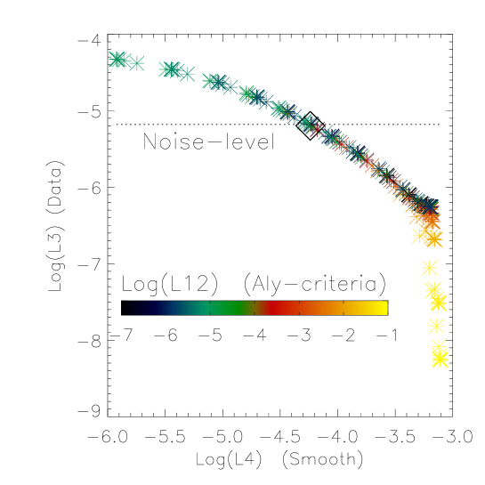
A survey of the $\mu$ parameters for one of the example computations (Low and Lou solution with noise model I) described in the next section shows that $\log(L_{3}(\mathbf{B}_{\mathrm{min}}))$ and $\log(L_{4}(\mathbf{B}_{\mathrm{min}}))$ are almost entirely determined by the ratio of $\mu_{3}$ to $\mu_{4}$ while $\log(L_{12}(\mathbf{B}_{\mathrm{min}}))$ depends on the absolute magnitude on $\mu_{3}$ and $\mu_{4}$. It is therefore convenient to display our results in a projection of the 3D phase space along the $\log(L_{12})$-axis as in Fig. 1. In this projection, the surface collapses nearly to a unique curve.

An obvious limiting value is obtained for $\mu_{3}$ $\rightarrow$ $\infty$ which yields $\mathbf{B}_{\mathrm{min}}$ = $\mathbf{B}_{\mathrm{obs}}$ with $L_{12}$ $\sim$ 10^-1, $L_{3}$ = 0 and $L_{4}$ $\sim$ 10^-3. For smaller values of $\mu_{3}$ we obtain a smoothed solution and, depending on $\mu_{4}$ also satisfy the Aly criteria much better than the original observational data. The price we have to pay is that $L_{3}$ attains finite values, which however is tolerable as long as $L_{3}$ does not exceed a noise value $L_{3}(\mathbf{B}_{\mathrm{noise}})$ (dotted line in Fig. 1). This value in our test case is known from the amount of noise added. For actual observations, it has to be estimated. The intersection of our solution surface with the noise level then defines the optimal ratio $\mu_{3}$ to $\mu_{4}$ (marked by a rhombus in Fig. 1. We choose both numbers small to enforce a good compliance with the Aly criteria, i.e., give much weight to $L_{12}$. This way, $L_{12}$ is reduced by 6 orders of magnitude, $\mathrm{B}$ is conveniently smoothed and yet it does not deviate from the observations by more than the instrument error. The smoothing will somewhat broaden prominent magnetic flux structures. A careful choice of the preprocessing parameters (as described above) ensures that the magnetic flux magnitudes and the corresponding magnetic field topology (which might become very complex for multiple magnetic sources, see [Schrijver and Title (2002)]) are not affected by the preprocessing.

4 Tests with the Low and Lou solution

Figure 2: The first row shows the original vector magnetogram deduced from the Low and Lou solution. In the second row we added noise (model I) to the solution to simulate measurement errors. In the bottom row we applied our preprocessing routine to the noisy data taken from the center row.

Figure 3: a) Some field lines for the original Low and Lou solution. b) Potential field reconstruction. c) Non-linear force-free reconstruction from noisy data (noise model I) without preprocessing. d) Non-linear force-free reconstruction from noisy data (noise model I) after preprocessing the vector magnetogram with our newly developed program. e) Non-linear force-free reconstruction from noisy data (noise model II) without preprocessing. f) Non-linear force-free reconstruction from noisy data (noise model II) after preprocessing. g) Non-linear force-free reconstruction from noisy data (noise model III) without preprocessing. h) Non-linear force-free reconstruction from noisy data (noise model III) after preprocessing the vector magnetogram with our newly developed program. The color coding shows the normal magnetic field component on the photosphere in all panel. One can see, that after preprocessing (panel d,f,h) the agreement with the original (a) is much better than without preprocessing (c,e,g).

For a first test we use the semi-analytic solution found by low:etal90. This solution has been designed in particular to test non-linear force-free extrapolation codes. The solution contains free parameters and we use $\Phi=\pi/2$ and $l=0.3$ (see low:etal90 for details). We extract the bottom boundary of this equilibrium and use it as input for our extrapolation code (see wiegelmann04). 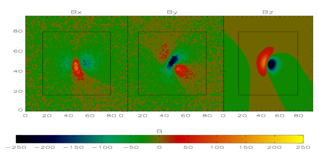This artificial vector magnetogram (see first row of Fig. 2) extrapolated from a semi-analytic solution is of course in perfect agreement with the assumption of a force-free field above (Aly-criteria) and the result of our extrapolation code showed a reasonable agreement with the original. Real measured vector magnetograms are not so ideal (and smooth) of course and we simulate this effect by adding noise to the Low and Lou magnetogram. We add noise to this ideal solution in the form
Noise model I:
$\delta B_{i}=n_{l}\cdot r_{n}\cdot\sqrt{B_{i}}$, where $n_{l}$ is the noise level and $r_{n}$ a random number in the range $-1\dots 1$. The noiselevel was choosen $n_{l}=5.0$ for the transversal magnetic field ($B_{x}$, $B_{y}$) and $n_{l}=0.25$ for $B_{z}$. This mimics a real magnetogram (see center row of Fig. 2) which has significantly higher noise in the transversal components of the magnetic field.
Noise model II:
$\delta B_{i}=n_{l}\cdot r_{n}$, where $n_{l}$ is the noise level and $r_{n}$ a random number in the range $-1\dots 1$. The noiselevel was choosen $n_{l}=10.0$ for the transversal magnetic field ($B_{x}$, $B_{y}$) and $n_{l}=0.5$ for $B_{z}$. This noise model adds an additive noise, independent from the magnetic field strength.
Noise model III:
$\delta B_{z}={\rm constant}$, ${\delta B_{t}}=\frac{\delta B_{{\rm tmin}}^{2}}{\sqrt{B_{t}^{2}+\delta B_{{\rm tmin}}^{2}}}$ where we choose the constant noise level of $B_{z}$ to $1$ and the minimum detection level $\delta B_{{\rm tmin}}=20$. This noise model mimics the effect that the transversal noise level is higher in regions with a low magnetic field strength, which is an immediate consequence of Eq. 4.

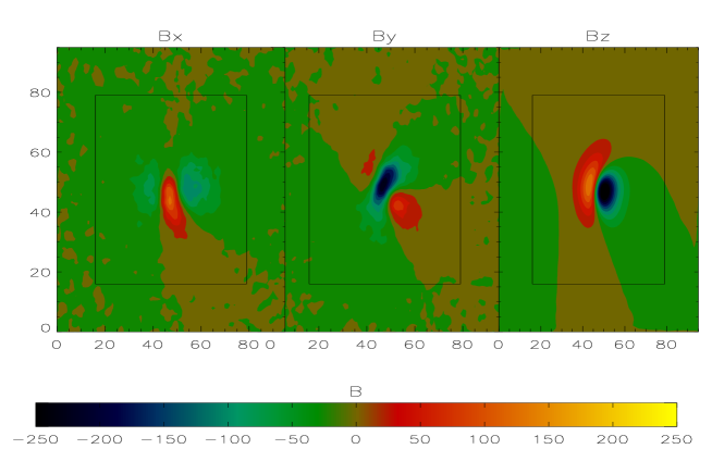
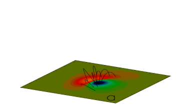
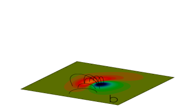
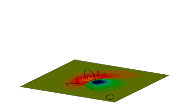
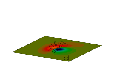
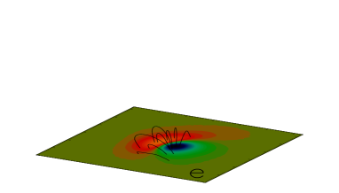
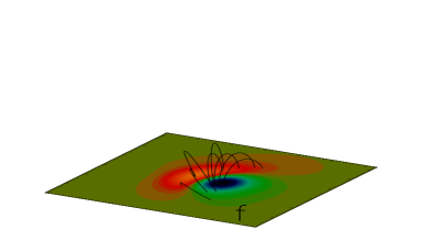
The bottom row of Fig. 2 shows the preprocessed vector magnetogram (for noise model I) after applying our procedure. The aim of the preprocessing is to use the resulting magnetogram as input for a non-linear force-free magnetic field extrapolation. Fig. 3 shows in panel a) the original Low and Lou solution and in panel b) a corresponding potential field reconstruction. In Fig. 3 we present only the central region of the whole magnetogram (marked with black rectangular box in Fig. 2 because the surrounding magnetogram is used as a boundary layer ($16$ grid points) for our non-linear force-free code (Our non-linear force-free code is explained in detail in wiegelmann04). The computation was done on a $96\times 96\times 80$ grid including a $16$ pixel boundary layer towards the lateral and top boundary of the computational box.) In the remaining panels of Fig. 3 we demonstrate the effect of the different noise models on the reconstruction. The noise levels were chosen so that the mean noise was similar for all three noise models. Fig. 3 c) shows a non-linear force-free reconstruction with noisy data (noise model I, magnetogram shown in the center panel of Fig. 2) and Fig. 3 d) presents a non-linear force-free reconstruction after preprocessing (Magnetogram shown in the bottom panel of Fig. 2). After preprocessing(Fig. 3 d) we get a much better agreement with the original solution (Fig. 3 a). Fig. 3 e) and f) show a non-linear force-free reconstruction for noise model II without (e) and after (f) preprocessing of the noisy data. Fig. 3 g) and h) show a non-linear force-free reconstruction for noise model III without (g) and after (h) preprocessing of the noisy data. Similar as for noise model I we find that the preprocessed data agree better with the original Fig. 3 a). We check the correlation of the original solution with our reconstruction with help of the vector correlation function $VC$ defined as

$$VC=\frac{\sum_{i}{\bf v_{i}}\cdot{\bf w_{i}}}{\sqrt{\sum_{i}|{\bf v_{i}}|^{2}}\;\sqrt{\sum_{i}|{\bf w_{i}}|^{2}}}.$$ (14)

${\bf v_{i}}$ correspond to a reference field (Low and Lou solution) and ${\bf w_{i}}$ to the non-linear force-free field reconstructed with our code.

Case	remark	preprocessing	vector correlation
a)	reference		1.00
b)	potential		0.85
c)	Noise model I	No	0.94
d)	Noise model I	Yes	0.98
e)	Noise model II	No	0.95
f)	Noise model II	Yes	0.98
g)	Noise model III	No	0.93
h)	Noise model III	Yes	0.98

The table confirms the visual inspection of Fig. 3. The correlation of the reconstructed magnetic field with the original becomes significantly improved after preprocessing of the data for all noise models. We knew already from previous studies [Wiegelmann and Neukirch (2003), Wiegelmann (2004)] that noise and inconsistencies in vector magnetograms have negative influence on the non-linear force-free reconstruction and the preprocessing routine described in this work tells us how to overcome these difficulties.

5 Application to data from the Solar Flare Telescope (SFT)

Figure 4: Top panel: vector magnetogram of AR 7321 taken with SFT at october, 26 1992. Bottom panel: After applying our preprocessing procedure. The resolution of the original SFT-magnetogram has been reduced by a factor of two to speed up the non-linear force-free magnetic field reconstruction. An inspection of the top and bottom panel shows that local small scale structures with strong flux density in the original lead to a broader structure with weaker flux density after preprocessing. Sharp boundaries between positive and negative flux regions are also broadened due to smoothing during preprocessing.

Figure 5: AR 7321 measured with SFT-data from october, 26 1992. a) Potential field reconstruction. b)Non-linear force-free reconstruction. The field lines start from the same footpoints within regions $B_{z}>0$ in both panels.

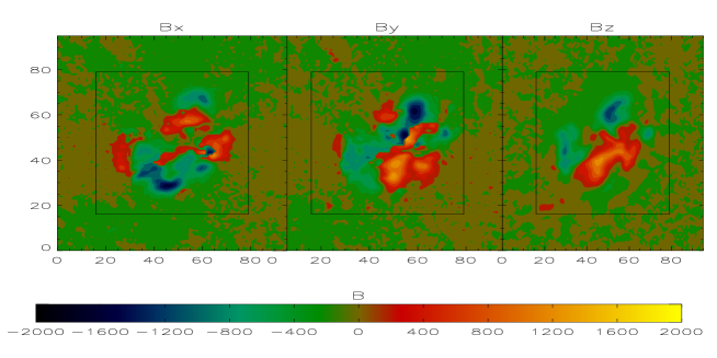
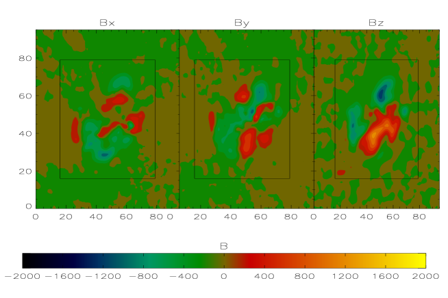
In this section we apply our method to vector magnetogram data of AR 7321 taken with SFT at the National Astronomical Observatory (NAO) in Tokyo. The SFT instrument is described in [Sakurai et al. (1995)] and the evolution of the photospheric magnetic field in AR 7321 has been studied by li:etal00b. The top panel of Fig. 4 shows the original data (original resolution reduced by a factor of two.) and the bottom panel after preprocessing. The structure of all components of the magnetic field is similar to the original. The magnetogram is almost flux-balanced ($\epsilon_{\mbox{flux}}=0.045$), but Aly’s criteria are not fulfilled in the original ($\epsilon_{\mbox{Aly}}=1.50$). After preprocessing we get $\epsilon_{\mbox{Aly}}=0.029$ and the data are also somewhat smoother than the original. The L-values of the original data and after preprocessing are: original preprocessed $L_{12}$ (Aly-criteria) $0.58$ $3.6\cdot 10^{-5}$ $L_{3}$ (Data) $0.0$ $1.0\cdot 10^{-5}$ $L_{4}$ (Smoothing) $2.1\cdot 10^{-4}$ $5.2\cdot 10^{-6}$

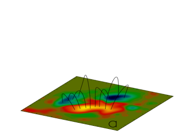
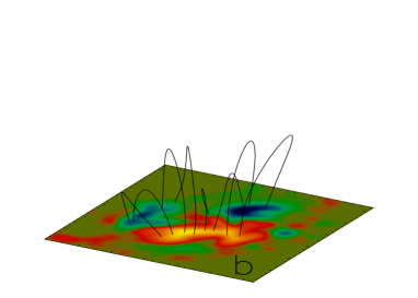
Fig. 5 a) shows a potential field reconstruction and Fig. 5 b) a non-linear force-free reconstruction based on the preprocessed vector magnetogram. The non-linear force-free computation was done in a $96\times 96\times 80$ box, including a boundary layer of $16$ grid points towards the lateral and top boundary. Fig. 5 shows only the center cube of $64\times 64\times 64$ pixel which corresponds to the area marked with a black rectangular box in Fig. 4.

6 Conclusions

Within this work we presented a method for the preprocessing of vector magnetogram data with the aim to use the result of the preprocessing as input for a non-linear force-free magnetic field extrapolation with help of an optimization code method. As a first test of the method we use the Low and Lou solution with overlaid noise with different noise models. A direct use of the noisy photospheric data for a non-linear force-free extrapolation showed no good agreement with the original Low and Lou solution, but after applying our newly developed preprocessing method we got a reasonable agreement with the original. The preprocessing method uses the high noise level in the transversal vector magnetogram components to drive the magnetogram towards boundary conditions which are consistent with the assumption of a force-free field above. To do so we use an minimization principle. On the one hand we control that the final boundary data are as close as possible (within the noise level) to the original measured data and on the other hand the data are forced to fulfill the Aly-criteria and be sufficiently smooth. Smoothness of the boundary data is required for the non-linear force-free extrapolation code, but also physically motivated because the magnetic field at the basis of the corona should be smoother than on the photosphere, where it is measured.

Let us remark that non-linear force-free extrapolations are only valid as long as the plasma $\beta$ is low and non-magnetic forces like pressure gradients and gravity can be neglected. This is usually the case in the corona (low $\beta$ plasma, $\beta\approx 10^{-4}$), but not in the photosphere ($\beta\approx 1$). A fully understanding on how the magnetic field evolves from the (non force-free) photosphere through the chromosphere and transition region into the (force-free) corona would require more advanced models, at least magnetohydrostatic equilibria. Measurements of the photospheric magnetic field vector are not sufficient for such models and one needs additional observations regarding plasma quantities (e.g. density, temperature, pressure). A magnetohydrostatic approach is also required to model prominences where the magnetic field counteracts the gravitational force of the material they support.

We apply our newly developed preprocessing program to data taken with the Solar Flare Telescope and use the preprocessed boundary data for a non-linear force-free field extrapolation.